Lecture 8 Objectives - eee.iub.edu.bd
51
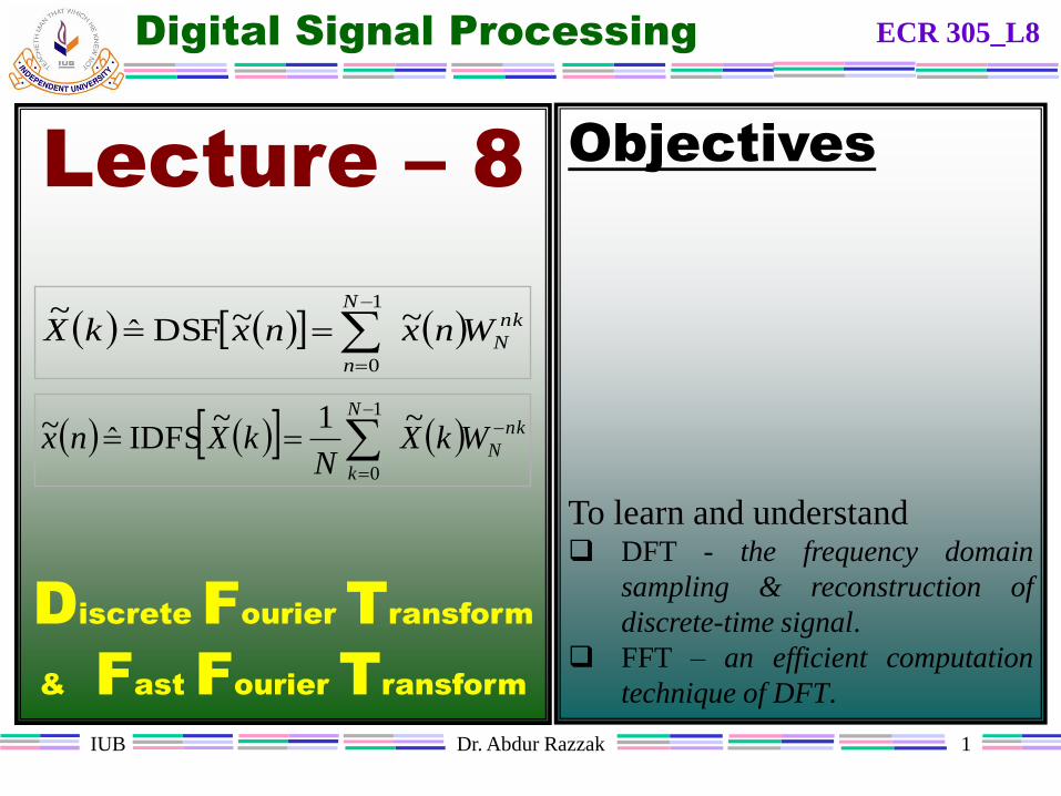
IUB Dr. Abdur Razzak 1 Digital Signal Processing Objectives To learn and understand DFT - the frequency domain sampling & reconstruction of discrete-time signal. FFT – an efficient computation technique of DFT. Lecture – 8 Discrete Fourier Transform & Fast Fourier Transform ECR 305_L8 nk N N n W n x n x k X ~ ~ DSF ˆ ~ 1 0 nk N N k W k X N k X n x ~ 1 ~ IDFS ˆ ~ 1 0
Transcript of Lecture 8 Objectives - eee.iub.edu.bd
IUB Dr. Abdur Razzak 1
Digital Signal Processing
Objectives
To learn and understand DFT - the frequency domain
sampling & reconstruction of
discrete-time signal.
FFT – an efficient computation
technique of DFT.
Lecture – 8
Discrete Fourier Transform
& Fast Fourier Transform
ECR 305_L8
nk
N
N
n
WnxnxkX ~~DSFˆ~ 1
0
nk
N
N
k
WkXN
kXnx
~1~
IDFSˆ~1
0
IUB Dr. Abdur Razzak 2
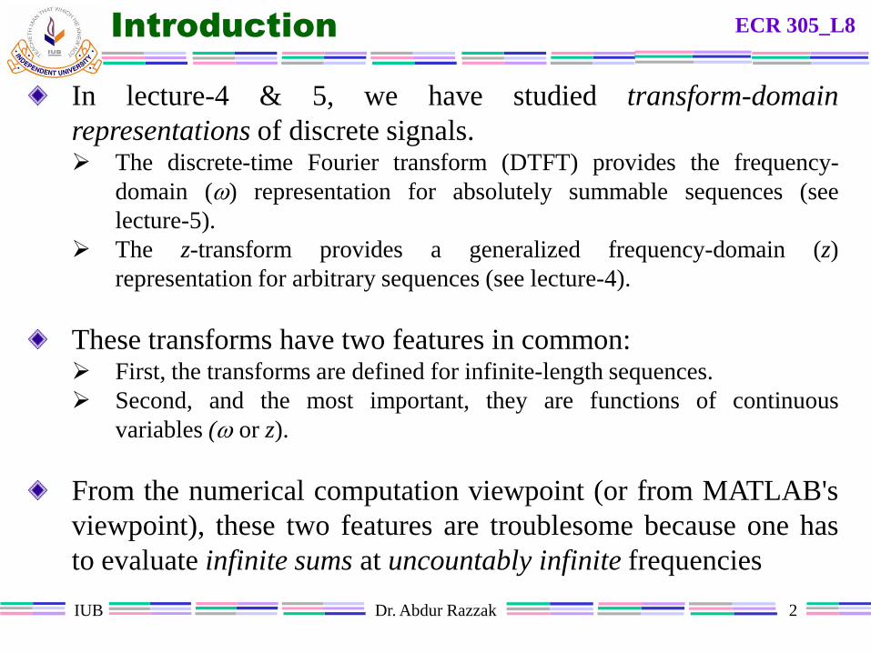
Introduction
In lecture-4 & 5, we have studied transform-domain
representations of discrete signals. The discrete-time Fourier transform (DTFT) provides the frequency-
domain () representation for absolutely summable sequences (see
lecture-5).
The z-transform provides a generalized frequency-domain (z)
representation for arbitrary sequences (see lecture-4).
These transforms have two features in common: First, the transforms are defined for infinite-length sequences.
Second, and the most important, they are functions of continuous
variables ( or z).
From the numerical computation viewpoint (or from MATLAB's
viewpoint), these two features are troublesome because one has
to evaluate infinite sums at uncountably infinite frequencies
ECR 305_L8
IUB Dr. Abdur Razzak 3
Introduction (contd..)
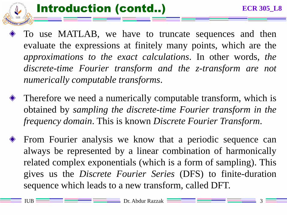
To use MATLAB, we have to truncate sequences and then
evaluate the expressions at finitely many points, which are the
approximations to the exact calculations. In other words, the
discrete-time Fourier transform and the z-transform are not
numerically computable transforms.
Therefore we need a numerically computable transform, which is
obtained by sampling the discrete-time Fourier transform in the
frequency domain. This is known Discrete Fourier Transform.
From Fourier analysis we know that a periodic sequence can
always be represented by a linear combination of harmonically
related complex exponentials (which is a form of sampling). This
gives us the Discrete Fourier Series (DFS) to finite-duration
sequence which leads to a new transform, called DFT.
ECR 305_L8

IUB Dr. Abdur Razzak 4
Discrete Fourier Series
Let us consider a periodic sequence
where N is the fundamental period of the sequence.
From Fourier analysis, we know that the periodic function can be
synthesized as a linear combinations of complex exponentials
whose frequencies are multiples (or harmonics) of the
fundamental frequency (which in our case is 2/N).
From the frequency-domain periodicity of the discrete-time
Fourier transform, we conclude that there are a finite number of
harmonics; the frequencies are { , k = 0, 1, 2,……, N–1}.
kNnxnx ~~
kN
2
ECR 305_L8
IUB Dr. Abdur Razzak 5
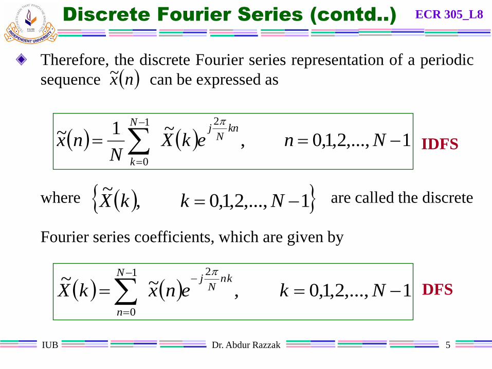
Discrete Fourier Series (contd..)
Therefore, the discrete Fourier series representation of a periodic
sequence can be expressed as
where are called the discrete
Fourier series coefficients, which are given by
1,...,2,1,0,~~21
0
NkenxkXnk
Nj
N
n
1,...,2,1,0,~1~
21
0
NnekXN
nxkn
Nj
N
k
nx~
1,...,2,1,0,~
NkkX
ECR 305_L8
IDFS
DFS
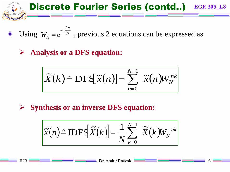
IUB Dr. Abdur Razzak 6
Discrete Fourier Series (contd..)
Using , previous 2 equations can be expressed as
Analysis or a DFS equation:
Synthesis or an inverse DFS equation:
Nj
N eW
2
nk
N
N
n
WnxnxkX ~~DFSˆ~ 1
0
nk
N
N
k
WkXN
kXnx
~1~
IDFSˆ~1
0
ECR 305_L8

IUB Dr. Abdur Razzak 7
Discrete Fourier Series (contd..)
In matrix form, the DFS and IDFS equations can be rewritten as
where the matrix called a DFS matrix given by
NNN xWX NNNNN
NXWXWx
*1- 1
211
11
10
1
1
111
N
N
N
N
N
NN
kn
NnkNN
WW
WWk
n
W
...
...::
...
...
ˆW ,
NW
ECR 305_L8
1-
1
0
Nx
x
x
N:
x
1
1
0
N
X
X
N
X
:X
IUB Dr. Abdur Razzak 8
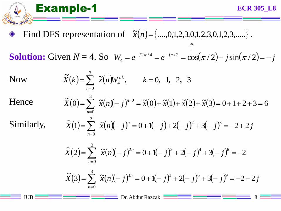
Example-1
Find DFS representation of .
Solution: Given N = 4. So
Now
Hence
Similarly,
,.....3,2,1,0,3,2,1,0,3,2,1,0....,~ nx
32104
3
0
,,,,~~
kWnxkX nk
n
jjeeW jj 2/sin2/cos2/4/2
4
632103~2~1~0~~0~ 0
3
0
xxxxjnxXn
n
jjjjjnxXn
n
223210~1~ 32
3
0
23210~2~ 6422
3
0
jjjjnxXn
n
jjjjjnxXn
n
223210~3~ 9633
3
0
ECR 305_L8
IUB Dr. Abdur Razzak 9
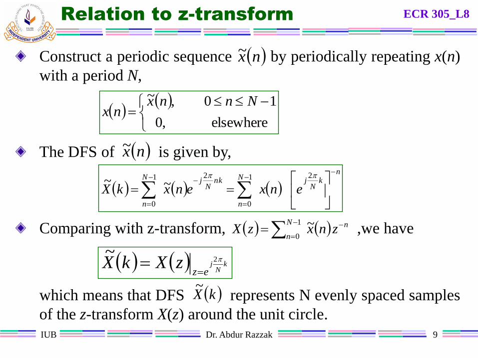
Relation to z-transform
Construct a periodic sequence by periodically repeating x(n)
with a period N,
The DFS of is given by,
Comparing with z-transform, ,we have
which means that DFS represents N evenly spaced samples
of the z-transform X(z) around the unit circle.
nx~
nx~
elsewhere
10
,0
,~
Nnnx
nx
n
kN
jN
n
nkN
jN
n
enxenxkX
21
0
21
0
~~
nN
nznxzX
~1
0
kN
j
ezzXkX 2
~
kX~
ECR 305_L8

IUB Dr. Abdur Razzak 10
Relation to DTFT
The DTFT of x(n) is given by
Comparing DFS & IDFS equations, we have
Let and , then the DFS
which means that the DFS is obtained by evenly sampling the
DTFT with the sampling interval .
njN
n
enxX
1
0
k
Nk
N
njN
n
nkN
jN
n
XenxenxkX
2
2
1
0
21
0
~~~
N
2ˆ1 1
2ˆ
kk
Nk
1 jkjeXeXkX k
ECR 305_L8

IUB Dr. Abdur Razzak 11
Discrete Fourier transform
The discrete Fourier series provided us a mechanism for numerically
computing the discrete-time Fourier transform. It also alerted us to a potential
problem of aliasing in the time domain.
Mathematics dictates that the sampling of the discrete-time Fourier transform
result in a periodic sequence x(n). But most of the signals in practice are not
periodic. They are likely to be of finite duration. How can we develop a
numerically computable Fourier representation for such signals?
Theoretically, we can take care of this problem by defining a periodic signal
whose primary shape is that of the finite-duration signal and then using the
DFS on this periodic signal.
Practically, we define a new transform called the Discrete Fourier Transform
(DFT), which is the primary period of the DFS. This DFT is the ultimate
numerically computable Fourier transform for arbitrary finite-duration
sequences.
ECR 305_L8

IUB Dr. Abdur Razzak 12
Discrete Fourier transform (contd..)
Discrete Fourier transform (DFT) of an N-point sequence:
or
Inverse discrete Fourier transform (IDFT) of an N-point
sequence:
elsewhere
10
,0
,~
DFTˆ
NkkX
nxkX
10,1
0
NkWnxkX nk
N
N
n
10,1~
1
0
NnWkXN
nx nk
N
N
k
ECR 305_L8
IUB Dr. Abdur Razzak 13
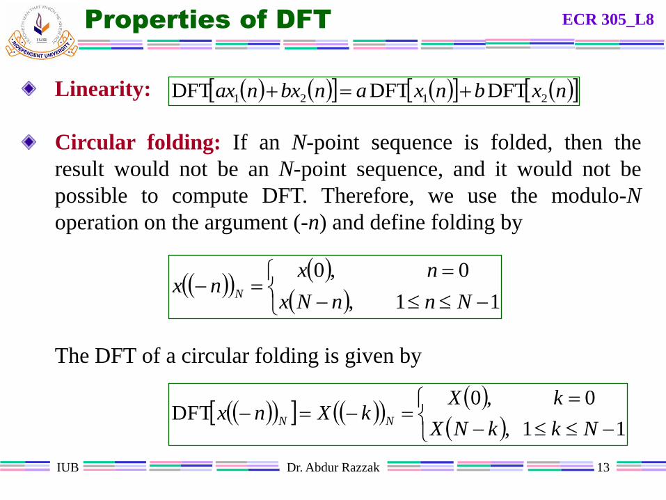
Properties of DFT
Linearity:
Circular folding: If an N-point sequence is folded, then the
result would not be an N-point sequence, and it would not be
possible to compute DFT. Therefore, we use the modulo-N
operation on the argument (-n) and define folding by
The DFT of a circular folding is given by
nxbnxanbxnax 2121 DFTDFTDFT
11
0
,
,0
Nn
n
nNx
xnx N
11
0
,
,0DFT
Nk
k
kNX
XkXnx NN
ECR 305_L8
IUB Dr. Abdur Razzak 14
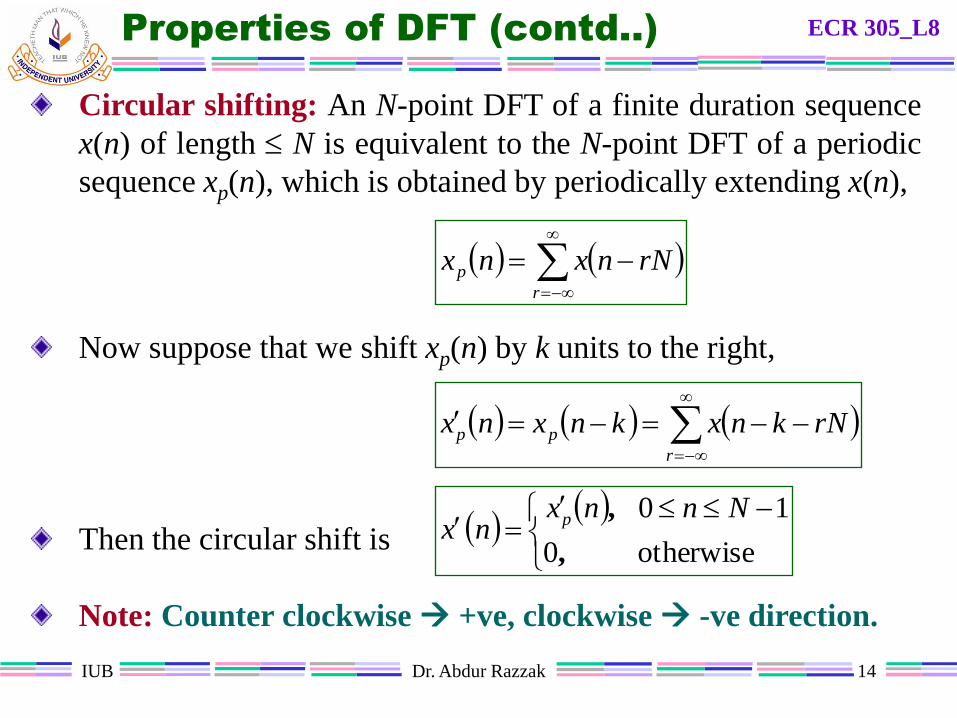
Properties of DFT (contd..)
Circular shifting: An N-point DFT of a finite duration sequence
x(n) of length N is equivalent to the N-point DFT of a periodic
sequence xp(n), which is obtained by periodically extending x(n),
Now suppose that we shift xp(n) by k units to the right,
Then the circular shift is
Note: Counter clockwise +ve, clockwise -ve direction.
r
p rNnxnx
ECR 305_L8
r
pp rNknxknxnx
otherwise
10
0
Nnnxnx
p
,
,

IUB Dr. Abdur Razzak 15
Properties of DFT (contd..)
Circular convolution: Consider 2 N-point sequences x1(n) and
x2(n). The respective N-point DFTs are
Then
Then the IDFT of X3(k), called the circular convolution, given by
ECR 305_L8
1210
2
1
1
0
1
NkenxkXnk
NjN
n
,...,,,,
1210
2
2
1
0
2
NkenxkXnk
NjN
n
,...,,,,
kXkXkX 213
1,...,2,1,01
0
213
NmnmxnxmxN
n
N

IUB Dr. Abdur Razzak 16
Example-2
Determine the circular shifting of the sequence by 2 units:
Solution:
ECR 305_L8
4321 ,,,nx

IUB Dr. Abdur Razzak 17
Example-2 (contd..) ECR 305_L8
IUB Dr. Abdur Razzak 18
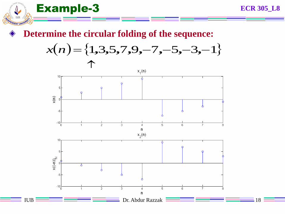
Example-3
Determine the circular folding of the sequence:
ECR 305_L8
135797531 ,,,,,,,,nx

IUB Dr. Abdur Razzak 19
Example-4
Determine the circular convolution of the following two
sequences:
Solution:
ECR 305_L8
12121 ,,,nx
43212 ,,,nx
1,...,2,1,0where
1
0
213
Nm
nmxnxmxN
n
N
16,14,16,143 mx

IUB Dr. Abdur Razzak 20
Example-4 (contd..) ECR 305_L8
1,...,2,1,0where
1
0
213
Nm
nmxnxmxN
n
N
16,14,16,143 mx
IUB Dr. Abdur Razzak 21
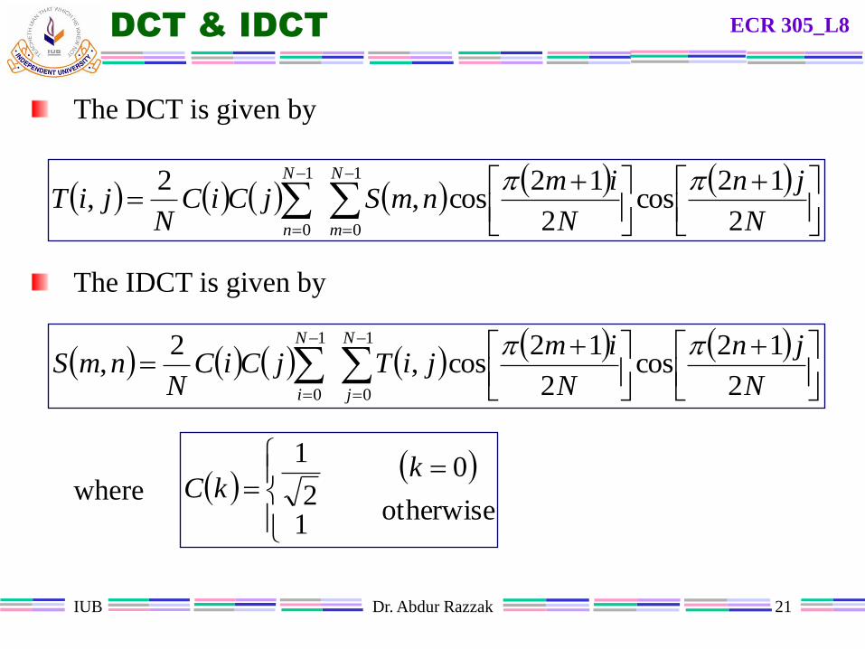
DCT & IDCT ECR 305_L8
The DCT is given by
The IDCT is given by
where
N
jn
N
imnmSjCiC
NjiT
N
m
N
n 2
12cos
2
12cos,
2,
1
0
1
0
otherwise
0
12
1
k
kC
N
jn
N
imjiTjCiC
NnmS
N
j
N
i 2
12cos
2
12cos,
2,
1
0
1
0
IUB Dr. Abdur Razzak 22
Fast Fourier Transform
Although DFT is a computable transform, the numerical
computation of the DFT is time consuming and its straightforward
implementation is very inefficient especially for large sequences.
Therefore, several algorithms have been developed to efficiently
compute the DFT. These are collectively called Fast Fourier
Transform (FFT) algorithms.
In 1965, Cooley and Tukey showed a procedure to substantially
reduce the amount of computations involved in the DFT, which
led to the explosion of the application of the DFT including in the
digital signal processing area and to the development of other
efficient algorithms. These are collectively known as Fast Fourier
Transform (FFT).
ECR 305_L8
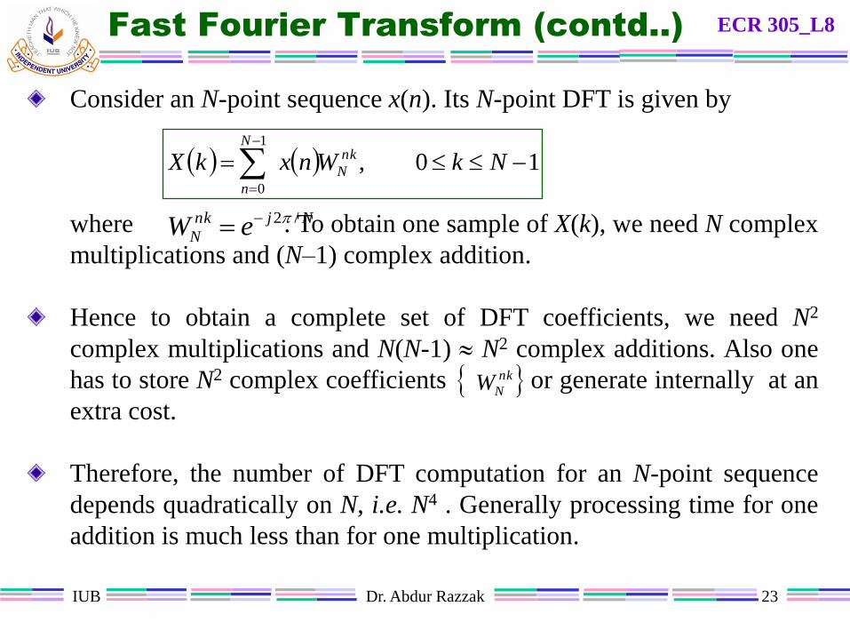
IUB Dr. Abdur Razzak 23
Fast Fourier Transform (contd..)
10,1
0
NkWnxkX nk
N
N
n
Consider an N-point sequence x(n). Its N-point DFT is given by
where . To obtain one sample of X(k), we need N complex
multiplications and (N–1) complex addition.
Hence to obtain a complete set of DFT coefficients, we need N2
complex multiplications and N(N-1) N2 complex additions. Also one
has to store N2 complex coefficients or generate internally at an
extra cost.
Therefore, the number of DFT computation for an N-point sequence
depends quadratically on N, i.e. N4 . Generally processing time for one
addition is much less than for one multiplication.
Njnk
N eW /2
nk
NW
ECR 305_L8

IUB Dr. Abdur Razzak 24
Fast Fourier Transform (contd..)
Goal of an efficient computation: In an efficiently designed
algorithm the number of computation should be constant per data
sample, and therefore the total number of computation should be
linear with respect to N.
The quadratic dependence of N can be reduced by realizing that
most of the computations (which are done again and again) can
be eliminated using the periodicity property
and the symmetry property
of the factor .
nk
N
Nnk
N WW 2/
Nkn
N
Nnk
N
nk
N WWW
nk
NW
ECR 305_L8
IUB Dr. Abdur Razzak 25
Example-5
Compute a 4-point DFT of x(n) = {1, 1, 1, 1} and develop an
efficient algorithm for its computation.
The above computation can be done in the matrix form
which requires 16 complex multiplications.
Efficient approach: Using periodicity
jeWkWnxkX jnk
n
4/2
44
3
0
;30,
3
2
1
0
3
2
1
0
9
4
6
4
3
4
0
4
6
4
4
4
2
4
0
4
3
4
2
4
1
4
0
4
0
4
0
4
0
4
0
4
x
x
x
x
WWWW
WWWW
WWWW
WWWW
X
X
X
X
jWWW
jWWWW
3
4
6
4
2
4
9
4
1
4
4
4
0
4
;1
;1
ECR 305_L8
IUB Dr. Abdur Razzak 26
Example-5 (contd..)
Putting these values into previous equation, we have
Using symmetry we obtain
3
2
1
0
11
1111
11
1111
3
2
1
0
x
x
x
x
jj
jj
X
X
X
X
21
21
21
21
312032103
312032102
312032101
312032100
hh
gg
hh
gg
xxjxxjxxjxxX
xxxxxxxxX
xxjxxjxxjxxX
xxxxxxxxX
ECR 305_L8

IUB Dr. Abdur Razzak 27
4-point DFT (contd..)
Hence an efficient algorithm is
These requires only 2 complex multiplications, which is a
considerably smaller number. A signal flow graph structure of
this algorithm is shown below:
212
211
212
211
331
220
131
020
21
jhhXxxh
ggXxxh
jhhXxxg
ggXxxg
stepstep
ECR 305_L8
IUB Dr. Abdur Razzak 28
Assignment-7 (due on next class)
Problems : 7.8, 7.12, 7.14, 7.17, 7.24, 7.25
ECR305_L8
IUB Dr. Abdur Razzak 29
MATLAB implementation
MATLAB
Examples
ECR 305_L8
IUB Dr. Abdur Razzak 30
MATLAB implementation of DFS
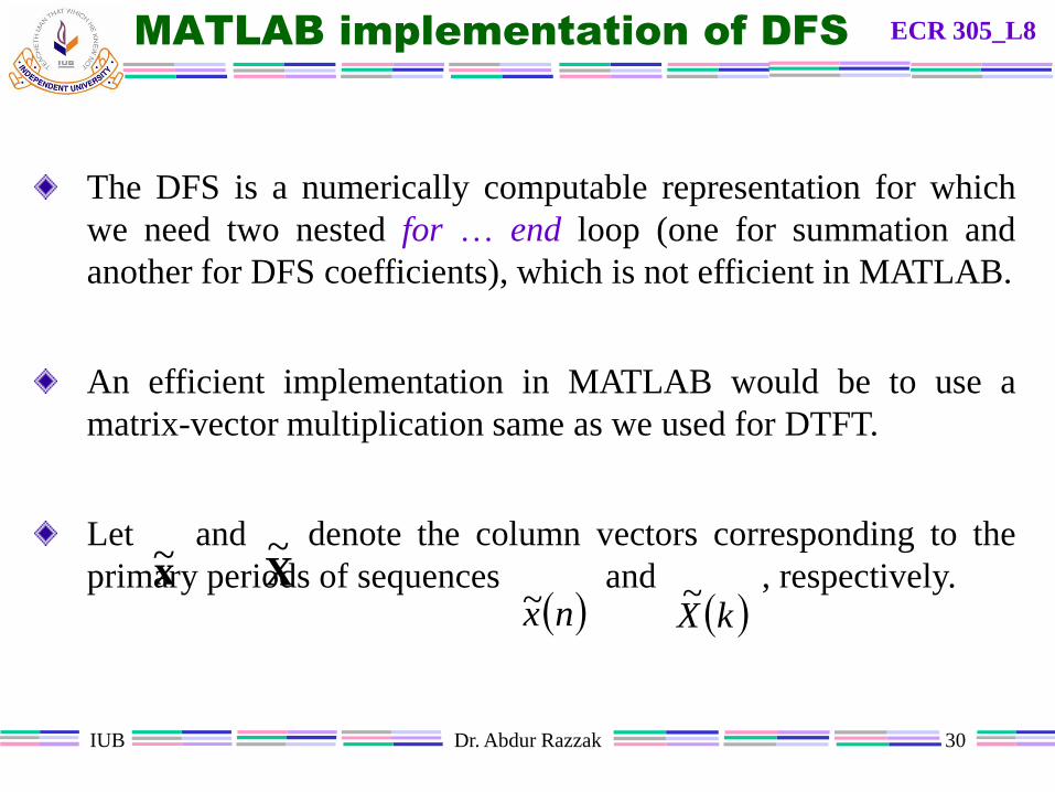
The DFS is a numerically computable representation for which
we need two nested for … end loop (one for summation and
another for DFS coefficients), which is not efficient in MATLAB.
An efficient implementation in MATLAB would be to use a
matrix-vector multiplication same as we used for DTFT.
Let and denote the column vectors corresponding to the
primary periods of sequences and , respectively.x~ X~
nx~ kX~
ECR 305_L8

IUB Dr. Abdur Razzak 31
MATLAB implementation of DFS (contd..)
Then DFS and IDFS equations can be rewritten as
where the matrix called a DFS matrix given by
xWX ~~N
XWx* ~1~N
N
211
11
1,0
...1
...::
...1
1...11
ˆ
N
N
N
N
N
NNkn
NnkNN
WW
WWk
n
WW
NW
ECR 305_L8
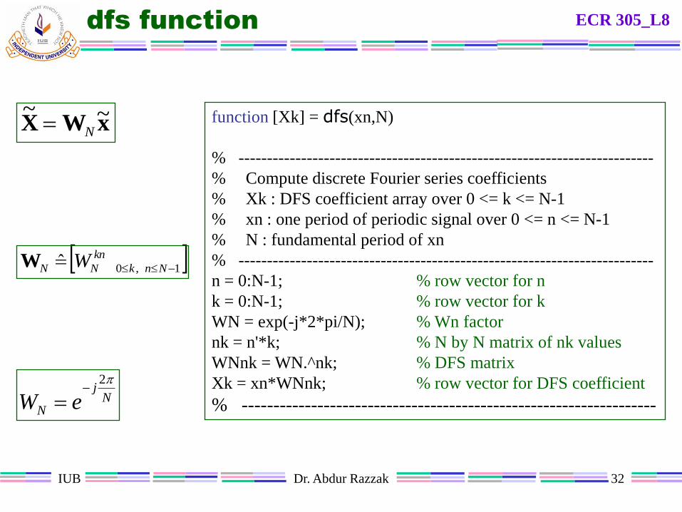
IUB Dr. Abdur Razzak 32
dfs function
function [Xk] = dfs(xn,N)
% -------------------------------------------------------------------------
% Compute discrete Fourier series coefficients
% Xk : DFS coefficient array over 0 <= k <= N-1
% xn : one period of periodic signal over 0 <= n <= N-1
% N : fundamental period of xn
% -------------------------------------------------------------------------
n = 0:N-1; % row vector for n
k = 0:N-1; % row vector for k
WN = exp(-j*2*pi/N); % Wn factor
nk = n'*k; % N by N matrix of nk values
WNnk = WN.^nk; % DFS matrix
Xk = xn*WNnk; % row vector for DFS coefficient
% ------------------------------------------------------------------N
j
N eW
2
xWX ~~N
kn
NnkNN W 1,0ˆ W
ECR 305_L8
IUB Dr. Abdur Razzak 33
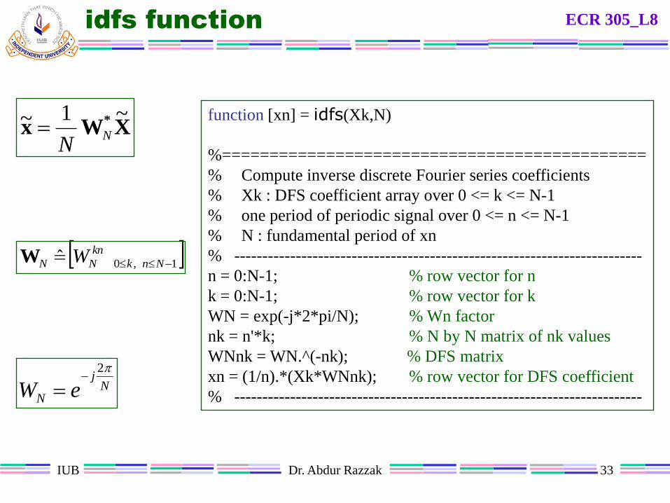
idfs function
Nj
N eW
2
kn
NnkNN W 1,0ˆ W
XWx* ~1~N
N
function [xn] = idfs(Xk,N)
%=============================================
% Compute inverse discrete Fourier series coefficients
% Xk : DFS coefficient array over 0 <= k <= N-1
% one period of periodic signal over 0 <= n <= N-1
% N : fundamental period of xn
% -------------------------------------------------------------------------
n = 0:N-1; % row vector for n
k = 0:N-1; % row vector for k
WN = exp(-j*2*pi/N); % Wn factor
nk = n'*k; % N by N matrix of nk values
WNnk = WN.^(-nk); % DFS matrix
xn = (1/n).*(Xk*WNnk); % row vector for DFS coefficient
% -------------------------------------------------------------------------
ECR 305_L8
IUB Dr. Abdur Razzak 34
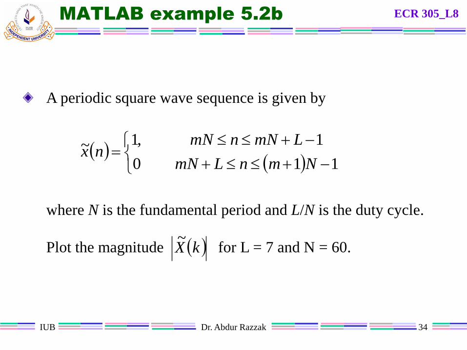
MATLAB example 5.2b
A periodic square wave sequence is given by
where N is the fundamental period and L/N is the duty cycle.
Plot the magnitude for L = 7 and N = 60.
11
1
0
,1~
NmnLmN
LmNnmNnx
kX~
ECR 305_L8
IUB Dr. Abdur Razzak 35
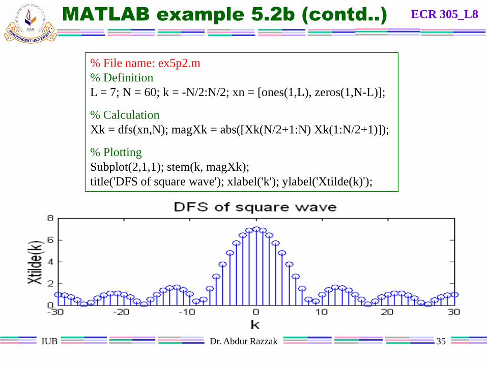
MATLAB example 5.2b (contd..)
% File name: ex5p2.m
% Definition
L = 7; N = 60; k = -N/2:N/2; xn = [ones(1,L), zeros(1,N-L)];
% Calculation
Xk = dfs(xn,N); magXk = abs([Xk(N/2+1:N) Xk(1:N/2+1)]);
% Plotting
Subplot(2,1,1); stem(k, magXk);
title('DFS of square wave'); xlabel('k'); ylabel('Xtilde(k)');
ECR 305_L8

IUB Dr. Abdur Razzak 36
MATLAB implementation of DFT
Then DFT and IDFT equations can be rewritten as
where the matrix called a DFT matrix given by
xWX N
XWx*
NN
1
211
11
1,0
...1
...::
...1
1...11
ˆ
N
N
N
N
N
NNkn
NnkNN
WW
WWk
n
WW
NW
ECR 305_L8

IUB Dr. Abdur Razzak 37
dft function
function [Xk] = dft(xn,N)
% -------------------------------------------------------------------------
% Compute discrete Fourier transform
% Xk : DFT coefficient array over 0 <= k <= N-1
% xn : N-point finite duration sequence
% N : Length of DFT
% -------------------------------------------------------------------------
n = 0:N-1; % row vector for n
k = 0:N-1; % row vector for k
WN = exp(-j*2*pi/N); % Wn factor
nk = n'*k; % N by N matrix of nk values
WNnk = WN.^nk; % DFT matrix
Xk = xn*WNnk; % row vector for DFT coefficient
% ------------------------------------------------------------------N
j
N eW
2
xWX N
kn
NnkNN W 1,0ˆ W
ECR 305_L8
IUB Dr. Abdur Razzak 38
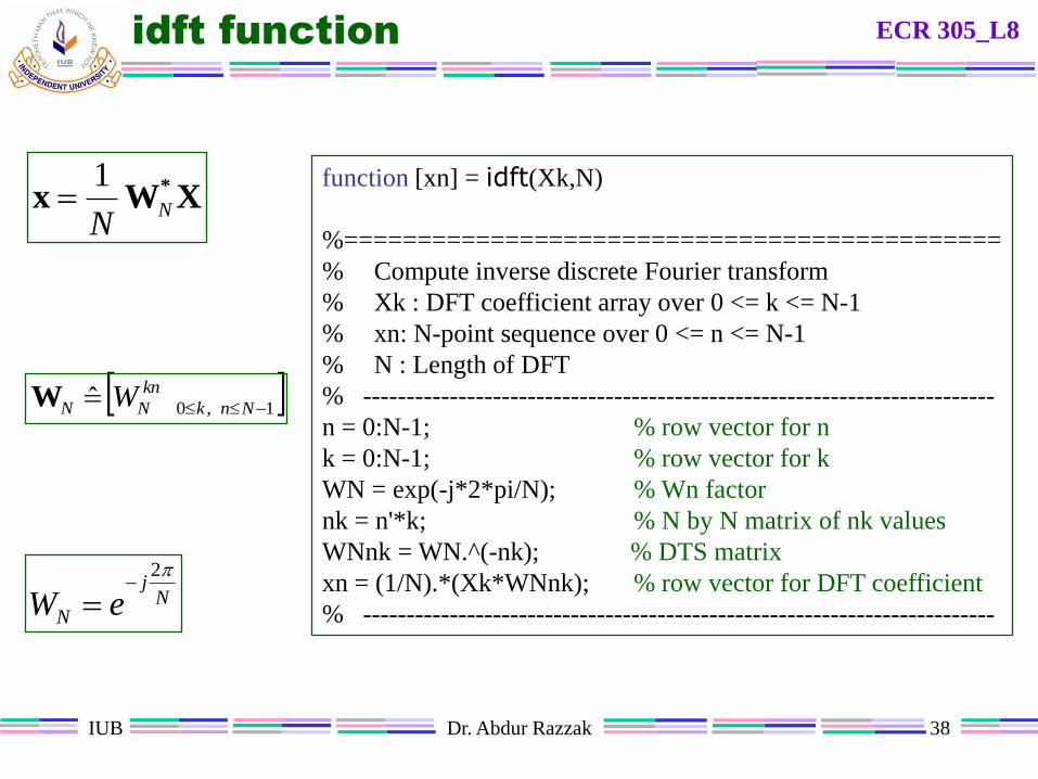
idft function
Nj
N eW
2
kn
NnkNN W 1,0ˆ W
XWx*
NN
1
function [xn] = idft(Xk,N)
%=============================================
% Compute inverse discrete Fourier transform
% Xk : DFT coefficient array over 0 <= k <= N-1
% xn: N-point sequence over 0 <= n <= N-1
% N : Length of DFT
% -------------------------------------------------------------------------
n = 0:N-1; % row vector for n
k = 0:N-1; % row vector for k
WN = exp(-j*2*pi/N); % Wn factor
nk = n'*k; % N by N matrix of nk values
WNnk = WN.^(-nk); % DTS matrix
xn = (1/N).*(Xk*WNnk); % row vector for DFT coefficient
% -------------------------------------------------------------------------
ECR 305_L8

IUB Dr. Abdur Razzak 39
MATLAB example 5.6
Let x(n) be an N-point sequence:
(a) Compute the DTFT and plot its magnitude and phase.
(b) Compute the 4-point DFT of x(n).
otherwise
30
,0
,1
n
nx
% Definition
n1=0; n2=3; n=n1:n2; M = 200; k = 0:M;
w=(4*pi/M)*k; N = 4; m = 0:N-1;
x = [1,1,1,1]; xn = [1,1,1,1];
% DTFT
X = dtft(x,n,k); magX=abs(X);
angX=angle(X)*180/pi;
% DFT
Xk = dft(xn,N); magXk = abs(Xk);
PhaXk = angle(Xk)*180/pi;
% Plotting
Subplot(2,1,1); stem(m,magXk);
title('Magnitude','fontsize',15);
xlabel('k','fontsize',15);
ylabel('X(k)','fontsize',15);
grid; hold on
plot(w/pi,magX,'--'); axis([0 4 0 5]);
Subplot(2,1,2); stem(m,PhaXk);
title('Angle','fontsize',15);
xlabel('k','fontsize',15);
ylabel('Degrees','fontsize',15);
grid; hold on
plot(w/pi,angX,'--'); axis([0 4 -200 200]);
ECR 305_L8

IUB Dr. Abdur Razzak 40
MATLAB example 5.6 (contd..) ECR 305_L8

IUB Dr. Abdur Razzak 41
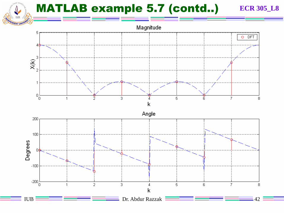
MATLAB example 5.7
How can we obtain further samples of X(ej)?
Ans:
% Definition
n1=0; n2=7; n=n1:n2; M = 200; k = 0:M;
w=(8*pi/M)*k; N = 8; m = 0:N-1;
x = xn = [ones(1,4),zeros(1,4)];
% DTFT
X = dtft(x,n,k); magX=abs(X);
angX=angle(X)*180/pi;
% DFT
Xk = dft(xn,N); magXk = abs(Xk);
PhaXk = angle(Xk)*180/pi;
% Plotting
Subplot(2,1,1); stem(m,magXk);
title('Magnitude','fontsize',15);
xlabel('k','fontsize',15);
ylabel('X(k)','fontsize',15);
grid; hold on
plot(w/pi,magX,'--'); axis([0 4 0 5]);
Subplot(2,1,2); stem(m,PhaXk);
title('Angle','fontsize',15);
xlabel('k','fontsize',15);
ylabel('Degrees','fontsize',15);
grid; hold on
plot(w/pi,angX,'--'); axis([0 4 -200 200]);
0,0,0,0,1,1,1,1nx <= By padding zeros
ECR 305_L8
IUB Dr. Abdur Razzak 42
MATLAB example 5.7 (contd..) ECR 305_L8

IUB Dr. Abdur Razzak 43
MATLAB example 5.7 (contd..)
How can we obtain further samples of X(ej)?
Ans:
0,0,0,0,0,0,0,0,0,0,0,0,1,1,1,1nx
ECR 305_L8

IUB Dr. Abdur Razzak 44
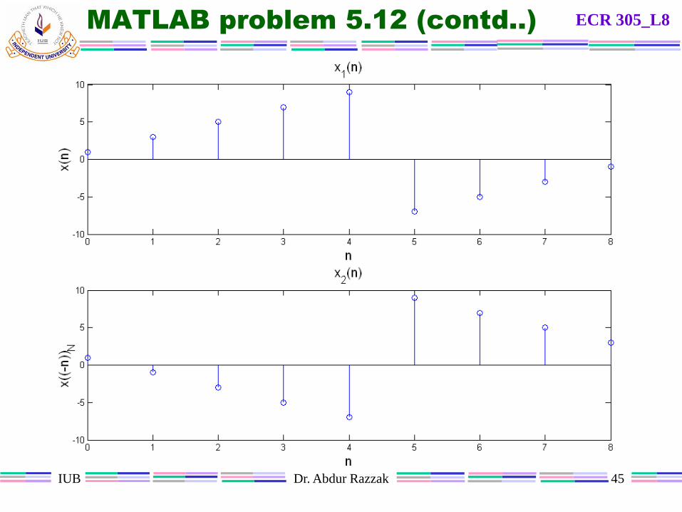
MATLAB problem 5.12
(a) Design a MATLAB function to implement an N-point circular
folding operation x2(n) = x1((-n))N.
(b) determine the circular folding of the sequence:
x1(n) = {1,3,5,7,9,-7,-5,-3,-1}
function x2 = circfold(x1,N)
n = 0:N-1;
x2 = x1(mod(-n,N)+1);
% Function
x1 = [1,3,5,7,9,-7,-5,-3,-1];
N = length(x1);
% Circular fold of x1
x2 = circfold(x1,N);
% Plotting
subplot(2,1,1)
stem(0:N-1,x1); title ('x_1(n)','fontsize',15);
xlabel('n','fontsize',15); ylabel('x(n)','fontsize',15);
subplot(2,1,2)
stem(0:N-1,x2); title ('x_2(n)','fontsize',15);
xlabel('n','fontsize',15);
ylabel('x((-n))_N','fontsize',15);
ECR 305_L8
IUB Dr. Abdur Razzak 45
MATLAB problem 5.12 (contd..) ECR 305_L8
IUB Dr. Abdur Razzak 46
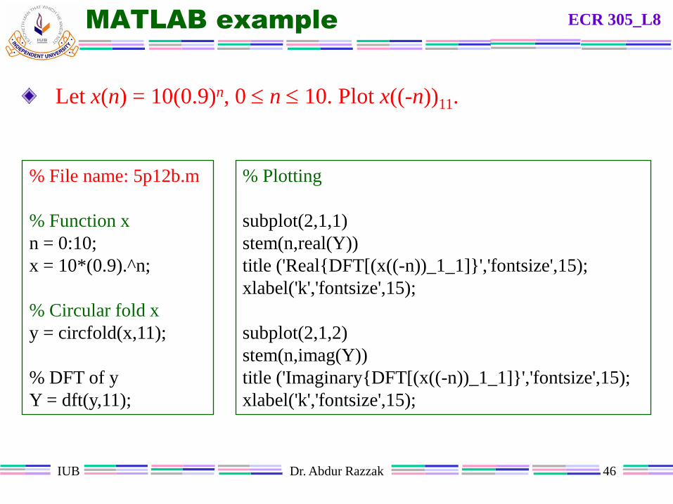
MATLAB example
Let x(n) = 10(0.9)n, 0 n 10. Plot x((-n))11.
% File name: 5p12b.m
% Function x
n = 0:10;
x = 10*(0.9).^n;
% Circular fold x
y = circfold(x,11);
% DFT of y
Y = dft(y,11);
% Plotting
subplot(2,1,1)
stem(n,real(Y))
title ('Real{DFT[(x((-n))_1_1]}','fontsize',15);
xlabel('k','fontsize',15);
subplot(2,1,2)
stem(n,imag(Y))
title ('Imaginary{DFT[(x((-n))_1_1]}','fontsize',15);
xlabel('k','fontsize',15);
ECR 305_L8

IUB Dr. Abdur Razzak 47
MATLAB example (contd..) ECR 305_L8

IUB Dr. Abdur Razzak 48
MATLAB example 5.6-fft
Let x(n) be an N-point sequence:
(a) Compute the DTFT and plot its magnitude and phase.
(b) Compute the 4-point DFT of x(n).
otherwise
30
,0
,1
n
nx
% File name: ex5p6fft.m
% Definition
N = 4; m = 0:N-1;
% Function
xn = [1,1,1,1];
% Calculation
Xk = fft(xn,N);
magXk = abs(Xk);
PhaXk = angle(Xk)*180/pi;
% Plotting
Subplot(2,1,1);
stem(m,magXk');
title('Magnitude','fontsize',15);
xlabel('k','fontsize',15);
ylabel('X(k)','fontsize',15);
Subplot(2,1,2);
stem(m,PhaXk');
title('Angle','fontsize',15);
xlabel('k','fontsize',15);
ylabel('Degrees','fontsize',15);
ECR 305_L8

IUB Dr. Abdur Razzak 49
MATLAB example 5.6-fft (contd..) ECR 305_L8
IUB Dr. Abdur Razzak 50
References
1. John G. Proakis, Digital Signal Processing, Pearson, 4th
Edition, Seventh Impression, 2011. (pp. 449–562)
2. Vinay K. Ingle, and John G. Proakis, Digital Signal
Processing using MATLAB, Thomson Learning
Bookware Companion Series, 2007. (pp. 118–185)
ECR 305_L8

IUB Dr. Abdur Razzak 51
Next class..
Digital Filter
Structure
ECR 305_L8