Lecture 8: Linear Programming

CS 506 Lecture: Linear Programming S’ 2020

Lecture 8: Linear Programming

Linear Programming: One of the most important computational problems in science and engineering islinear programming, or LP for short. LP is perhaps the simplest and best known example of multi-dimensional constrained optimization problems. In constrained optimization, the objective is to finda point in d-dimensional space that minimizes (or maximizes) a given objective function, subject tosatisfying a set of constraints on the set of allowable solutions. LP is distinguished by the fact that boththe constraints and objective function are linear functions. In spite of this apparent limitation, linearprogramming is a very powerful way of modeling optimization problems. Typically, linear programmingis performed in spaces of very high dimension (hundreds to thousands or more). There are, however, anumber of useful (and even surprising) applications of linear programming in low-dimensional spaces.

Formally, in linear programming we are given a set of linear inequalities, called constraints, in reald-dimensional space Rd. Given a point (x1, . . . , xd) 2 Rd, we can express such a constraint as a1x1 +. . . + adxd b, by specifying the coecient ai and b. (Note that there is no loss of generality inassuming that the inequality relation is , since we can convert a relation to this form by simplynegating the coecients on both sides.) Geometrically, each constraint defines a closed halfspace inRd. The intersection of these halfspaces intersection defines a (possibly empty or possibly unbounded)polyhedron in Rd, called the feasible polytope

5 (see Fig. 41(a)).

(a)

feasiblepolytope

feasiblepolytope

c

optimalvertex

(b)

Fig. 41: 2-dimensional linear programming.

We are also given a linear objective function, which is to be minimized or maximized subject to thegiven constraints. We can express such as function as c1x1+ . . .+cdxd, by specifying the coecients ci.(Again, there is no essential di↵erence between minimization and maximization, since we can simplynegate the coecients to simulate the other.) We will assume that the objective is to maximize theobjective function. If we think of (c1, . . . , cd) as a vector in Rd, the value of the objective function isjust the projected length of the vector (x1, . . . , xd) onto the direction defined by the vector c. It is nothard to see that (assuming general position), if a solution exists, it will be achieved by a vertex of thefeasible polytope, called the optimal vertex (see Fig. 41(b)).

5To some geometric purists this an abuse of terminology, since a polytope is often defined to be a closed, bounded convexpolyhedron, and feasible polyhedra need not be bounded.

Lecture Notes 45 CMSC 754

Figure 1. Left: The feasible polytope is defined by multiple half-planes; Right: Goal is to find optimal vertex in the feasiblepolytope that is furthest in the direction of the objective function vector c.

Note: These lecture notes are based on the textbook “Computational Geometry” by Berg et al.;lecture notes from [1]; and lecture notes from MIT 6.854J Advanced Algorithms class by M. Goe-mans

1 The Linear Programming Problem

In linear programming (LP), we want to find a point in d dimensional space that minimizes a givenlinear objective function subject to a set of linear constraints. Frequently, LP is done in 100’s or1, 000’s of dimensions, but many applications occur in low-dimensional spaces.

Formally, we’re given a set of linear inequalities, called constraints in Rd. Given a point(x1, . . . xd) ∈ Rd, we can express a constraint as a1x1 + . . . adxd ≤ b, by specifying coefficientsai, b ∈ R.1 Each constraint defines a halfspace in Rd and the intersection of halfspaces defines a(possibly empty or unbounded) polytope called the feasible polytope.

Next we’re given a linear objective function to be maximized. Given a point x ∈ Rd, we expressthe objective function as c1x1 + . . . cdxd, for coefficients ci.

2 We can think of the coefficients as avector c ∈ Rd, and then the value of the objective function for x ∈ Reald is just x · c. Assuminggeneral position, it’s not hard to see that if a solution exists, it’ll be achieved by a vertex of thefeasible polytope. See Figure 1.

In general, a d-dimensional LP can be expressed as.

Maximize: c1x1 + c2x2 + . . . cdxd.Subject to:

a1,1x1 + . . . a1,dxd ≤ b1

a2,1x1 + . . . a2,dxd ≤ b2

. . .

an,1x1 + . . . an,dxd ≤ bn

1Note that there is no loss in generality by assuming ≤ constrains, since we can convert a ≥ to this form by simplymultiplying the inequality by −1.

2Again there is no difference between minimization or maximization since we can negate the coefficients to gofrom one to the other.

1


In general, a d-dimensional linear programming problem can be expressed as:

Maximize: c1x1 + c2x2 + · · ·+ cdxd

Subject to: a1,1x1 + · · ·+ a1,dxd b1a2,1x1 + · · ·+ a2,dxd b2...an,1x1 + · · ·+ an,dxd bn,

where ai,j , ci, and bi are given real numbers. This can be also be expressed in matrix notation:

Maximize: cTx,Subject to: Ax b.

where c and x are d-vectors, b is an n-vector and A is an nd matrix. Note that c should be a nonzerovector, and n should be at least as large as d and may generally be much larger.

There are three possible outcomes of a given LP problem:

Feasible: The optimal point exists (and assuming general position) is a unique vertex of the feasiblepolytope (see Fig. 42(a)).

Infeasible: The feasible polytope is empty, and there is no solution (see Fig. 42(b)).

Unbounded: The feasible polytope is unbounded in the direction of the objective function, and sono finite optimal solution exists (see Fig. 42(c)).

feasiblepolytope

optimal

c c

vertex

c

optimum

(a) (b) (c)

feasible infeasible unbounded

Fig. 42: Possible outcomes of linear programming.

In our figures (in case we don’t provide arrows), we will assume the feasible polytope is the intersectionof upper halfspaces. Also, we will usually take the objective vector c to be a vertical vector pointingdownwards. (There is no loss of generality here, because we can always rotate space so that c is parallelany direction we like.) In this setting, the problem is just that of finding the lowest vertex (minimumy-coordinate) of the feasible polytope.

Linear Programming in High Dimensional Spaces: As mentioned earlier, typical instances of linearprogramming may involve hundreds to thousands of constraints in very high dimensional space. It canbe proved that the combinatorial complexity (total number of faces of all dimensions) of a polytopedefined by n halfspaces can be as high as (nbd/2c). In particular, the number of vertices alone mightbe this high. Therefore, building a representation of the entire feasible polytope is not an ecientapproach (except perhaps in the plane).

The principal methods used for solving high-dimensional linear programming problems are the simplex

algorithm and various interior-point methods. The simplex algorithm works by finding a vertex on


Figure 2. Possible Outcomes of a LP

where x1, . . . xd are the d variables,and ai,j , ci and bi are given real numbers. This can be writtenin matrix notation as

Maximize: cTx,Subject to: Ax ≤ b

Here c and x are d-vectors, b is an n and A is a n by d matrix, where n is the number of constraints.Note that n should be at least as large as d.

There are three possible outcomes for a given LP problem. See Figure 2Feasible: An optimal point exists and (assuming general position) is a unique vertex of the feasiblepolytope.InFeasible: The feasible polytope is empty and there is no solution

Unbounded: The feasible polytope is unbounded in the direction of c and so no finite optimal

solution exists.

2 Solving LP in Constant Dimensions

We now discuss the incremental construction method for efficiently solving LP in constant di-mensions. There are other methods for general LP (such as the interior point method). Thesealgorithms have weakly polynomial time in that they are polynomial in the number of bits of the in-put. (This is in contrast to strongly polynomial time algorithms that are polynomial in the numberof values (i.e. numbers) in the input, not in their size).

Incremental construction is a technique that is frequently used in computational geometry.

2.1 Initialization

Recall that we are given n halfspaces h1, . . . hd in Rd, and an objective vector c, and we want tocompute the vertex of the feasible polytope that is the most extreme in the direction of c.

We will initially assume that the LP is bounded and that we have d halfspaces that provide uswith an initial feasible point. Our approach will be to add halfspaces one at a time and successivelyupdate this feasible point.

Finding a set of initial d bounding halfplanes is non-trivial. Assume that there is some maximumvalue M that any variable can take on. The we add d constraints of the following form for allvariables1 ≤ i ≤ d xi ≤ M if ci > 0, and −xi ≤ M otherwise. These will be our initial d constraints. Laterwe will show how to also handle unbounded LPs. See Figure 3 left.

2


the feasible polytope, then walking edge by edge downwards until reaching a local minimum. (Byconvexity, any local minimum is the global minimum.) It has been long known that there are instanceswhere the simplex algorithm runs in exponential time, but in practice it is quite ecient.

The question of whether linear programming is even solvable in polynomial time was unknown untilKhachiyan’s ellipsoid algorithm (late 70’s) and Karmarkar’s more practical interior-point algorithm(mid 80’s). Both algorithms are polynomial in the total number of bits needed to describe the input.This is called a weakly polynomial time algorithm. It is not known whether there is a strongly poly-nomial time algorithm, that is, one whose running time is polynomial in both n and d, irrespective ofthe number of bits used for the input coecients. Indeed, like P versus NP, this is recognized by someas one of the great unsolved problems of mathematics.

Solving LP in Spaces of Constant Dimension: There are a number of interesting optimization prob-lems that can be posed as a low-dimensional linear programming problem. This means that the numberof variables (the xi’s) is constant, but the number of constraints n may be arbitrarily large.

The algorithms that we will discuss for linear programming are based on a simple method calledincremental construction. Incremental construction is among the most common design techniques incomputational geometry, and this is another important reason for studying the linear programmingproblem.

(Deterministic) Incremental Algorithm: Recall our geometric formulation of the LP problem. We aregiven n halfspaces h1, . . . , hd in Rd and an objective vector c, and we wish to compute the vertexof the feasible polytope that is most extreme in direction c. Our incremental approach will be basedon starting with an initial solution to the LP problem for a small set of constraints, and then we willsuccessively add one new constraint and update the solution.

In order to get the process started, we need to assume (1) that the LP is bounded and (2) we can finda set of d halfspaces that provide us with an initial feasible point. Getting to this starting point isactually not trivial.6 For the sake of focusing on the main elements of the algorithm, we will skip thispart and just assume that the first d halfspaces define a bounded feasible polytope (actually it will bea polyhedral cone). The the unique point where all d bounding hyperplanes, h1, . . . , hd, intersect willbe our initial feasible solution. We denote this vertex as vd (see Fig. 43(a)).

c

h1h2

v2c

vi1

vi?

hi

(a)

vi = vi1

`i

(b) (c)

c

hi

Fig. 43: (a) Starting the incremental construction and (b) the proof that the new optimum lies on `i.

We will then add halfspaces one by one, hd+1, hd+2, . . ., and with each addition we update the cur-rent optimum vertex, if necessary. Let vi denote the optimal feasible vertex after the addition ofh1, h2, . . . , hi. Notice that with each new constraint, the feasible polytope generally becomes smaller,and hence the value of the objective function at optimum vertex can only decrease. (In terms of ourillustrations, the y-coordinate of the feasible vertex increases.)

6Our textbook explains how to overcome these assumptions in O(n) additional time.


Figure 3. Left: Starting the incremental construction; Right: Proof that new optimum lies on ℓi

Note that if one of these “max value” constraints turns out to intersect the point that iseventually output, then we know that the original LP is unbounded. In this way, we can detectunbounded LPs also.

Additionally, we’ll assume that there is a unique solution, which we call the optimal vertex.This follows via the general position assumption (or by rotating the plane slightly).

2.2 Incremental Algorithm

We can imagine adding the halfspaces hd+1, hd+2, . . . and with each addition, update the currentoptimum vertex if necessary. Note that the feasible polytope gets smaller with each halfplaneaddition and so the value of the objective function can only decrease. In Figure 4, the y-coordinateof the feasible vertex decreases.

Let vi be the current optimum vertex after halfplane hi is added. There are two cases that canoccur when hi is added. In the easy case, vi−1 lies in the halfspace hi, and so already satisfies theconstraint. Thus vi = vi−1.

In the hard case, vi−1 is not in the halfplane hi, i.e. it violates the constraint. In this case, thefollowing lemma shows that vi must lie on the hyperplane that bounds hi.

Lemma 1. After addition of halfplane hi, if the LP is still feasible but vi ∕= vi−1, then vi lies onthe hyperplane bounding hi.

Proof: Let ℓi denote the bounding hyperplane for hi. By way of contradiction, suppose vi doesnot lie on ℓi (see Figure 3). Now consider the line segment between vi−1 and vi. First note thatthis line segment must cross ℓi since vi is in hi and vi−1 is not. Further, the entire segment is in theregion bounded by the first i− 1 hyperplanes, and so by convexity, the part of the segment that isin hi is in the region bounded by the first i hyperplanes.

Next, note that the objective function is maximized on this line segment at the point vi−1.Also, since the objective function is linear, it must be non-decreasing as we move from vi to vi−1.Thus, there is a point on ℓi with objective function at least equal to vi. But this contradicts theuniqueness property, so vi must be on ℓi.

2.3 Recursively updating vi

Consider the case where vi−1 does not lie in hi (Figure 4, left). Again, let ℓi denote the hyperplanebounding hi. We basically project everything onto that hyperplane and solve a d− 1 dimensionalLP. In particular, we first project c onto ℓi to get the vector c′ (Figure 4, right). Next intersecteach of the halfspaces h1, . . . hi−1 with ℓi. Each projection in a d − 1 dimensional halfspace thatlies on ℓi. Finally, since ℓi is a d − 1 dimensional hyperplane, we can project ℓi onto Rd−1 with a

3


There are two cases that can arise when hi is added. In the first case, vi1 lies within the halfspace hi,and so it already satisfies this constraint (see Fig. 43(b)). If so, then it is easy to see that the optimumvertex does not change, that is vi = vi1.

In the second case vi1 violates constraint hi. In this case we need to find a new optimum vertex(see Fig. 44(c)). Let us consider this case in greater detail. The key observation is presented in thefollowing claim, which states that whenever the old optimum vertex is infeasible, the new optimumvertex lies on the bounding hyperplane of the new constraint.

Lemma: If after the addition of constraint hi the LP is still feasible but the optimum vertex changes,then the new optimum vertex lies on the hyperplane bounding hi.

Proof: Let ì denote the bounding hyperplane for hi. Let vi1 denote the old optimum vertex.Suppose towards contradiction that the new optimum vertex vi does not lie on ì (see Fig. 43(c)).Consider the directed line segment vi1vi. Observe first that as you travel along this segmentthe value of the objective function decreases monotonically. (This follows from the linearity ofthe objective function and the fact that vi1 is no longer feasible.) Also observe that, because itconnects a point that is infeasible (lying below ì) to one that is feasible (lying strictly above ì),this segment must cross ì. Thus, the objective function is maximized at the crossing point itself,which lies on ì, a contradiction.

Recursively Updating the Optimum Vertex: Using this observation, we can reduce the problem offinding the new optimum vertex to an LP problem in one lower dimension. Let us consider an instancewhere the old optimum vertex vi1 does not lie within hi (see Fig. 44(a)). Let ì denote the hyperplanebounding hi. We first project the objective vector c onto ì, letting c0 be the resulting vector (seeFig. 44(b)). Next, intersect each of the halfspaces h1, . . . , hi1 with ì. Each intersection is a (d1)-dimensional halfspace that lies on ì. Since ì is a (d 1)-dimensional hyperplane, we can project ìonto Rd1 space (see Fig. 44(b)). We will not discuss how this is done, but the process is a minormodification of Gauss elimination in linear algebra. We now have an instance of LP in Rd1 involvingi 1 constraints. We recursively solve this LP. The resulting optimum vertex vi is then projected backonto ì and can now be viewed as a point in d-dimensional space. This is the new optimum point thatwe desire.

vi1

chi

vivi

(a) (b)

ì ì c0intersect with ì

c0

project onto Rd1

Fig. 44: Incremental construction.

The recursion ends when we drop down to an LP in 1-dimensional space (see Fig. 44(b)). The projectedobjective vector c0 is a vector pointing one way or the other on the real line. The intersection of eachhalfspace with ì is a ray, which can be thought of as an interval on the line that is bounded on oneside and unbounded on the other. Computing the intersection of a collection of intervals on a line canbe done easily in linear time, that is, O(i 1) time in this case. (This interval is the heavy solid line inFig. 44(b).) The new optimum is whichever endpoint of this interval is extreme in the direction of c0.If the interval is empty, then the feasible polytope is also empty, and we may terminate the algorithm


Figure 4. Projection during the incremental construction.

1-to-1 mapping. Then we apply this mapping to all the other vectors to get a LP in Rd−1 withi− 1 constraints.

Algebraically, the way we can do this is simply to set the constraint associated with ℓi to equalityand then remove a variable and a constraint from the LP. For example, if the constraint associatedwith ℓi is x1 + 2x2 − 3x3 ≤ 5. Then we set x1 = 5− 2x2 + 3x3, do a substitution in the LP usingthis equation wherever we see the variable x1 and then remove the variable x1 from the LP. Wecan do all this in O(di) time.

2.4 Base Case

The recursion ends when we get an LP in 1-dimensional space. Then the projected objective vectorjust points one way or the other on the real line; the intersection of each half-space with ℓi is a ray.Computing the intersection of a collection of rays on the line can be done in linear time. (This isthe heavy solid line in Figure 4, right). The new optimum is whichever endpoint of this intervalis most extreme in the direction of c′. If the interval is empty, then the feasible polytope is alsoempty. So when d = 1, we can solve the LP over i halfplanes in O(i) time.

2.5 Worst-Case Analysis

Let T (d, n) be the runtime for the LP with n constraints in d dimensional space. For simplicity, wewill analyze the recursive algorithm where we remove a constraint, recursively solve the LP, andthen either return the recursive solution or project onto the constraint. Then we get the followinganalysis.

What is T (d, n)? If xn−1 satisfies the removed constraint (which takes O(d) time to check),we’re done. If not, we reduce the LP to only d− 1 variables in O(dn) time (O(d) time to eliminatethe variable in each constraint). So, in the worst case, we get

T (d, n) = T (d, n− 1) +O(dn) + T (d− 1, n− 1)

Unfortunately, the solution to this recurrence is Θ(nd).

2.6 Randomization to the Rescue

Note that the above analysis assumes we always require a projection, and that we never get thelucky case where vi−1 is in hi. If we first randomly permute the hyperplanes, we can calculatethe probability of the “lucky” and “unlucky” cases to get an expected runtime. Let pi be theprobability that there is no change to vi−1. Then the expected runtime is given by the recurrencerelation:

4


• On the other hand, if any of them were the last to be inserted, then vi did not exist yet, andhence the optimum must have changed as a result of this insertion. (As is the case in Fig. 45(c),where h7 is the last to be inserted.)

c

(a)

vi

h5

h4

h7h6

h3

h1

h3

h2c

(b)

vi vi1

h5

h4

h6

h3

h1

h3

h2c

(c)

vi = vi1

h4

h7h6

h3

h1

h3

h2

h7

h5

Fig. 45: Backwards analysis for the randomized LP algorithm.

Thus, the optimum changes if and only if either one of the d defining halfspaces was the last halfspaceinserted. Since all of the i halfspaces are equally likely to be last, this happens with probability d/i.Therefore, pi = d/i.

This probabilistic analysis has been conditioned on the assumption that Si was the subset of halfspaceseen so far, but since the final probability does not depend on any properties of Si (just on d and i),the probabilistic analysis applies unconditionally to all subsets of size i.

Returning to our analysis, since pi = d/i, and applying the induction hypothesis that Td1(i) =d1(d 1)! i, we have

Td(n) nX

i=d+1

d+ pi

di+ Td1(i)

nX

i=d+1

d+

d

i

di+ d1(d 1)! i

nX

i=d+1

(d+ d2 + d1d!) (d+ d2 + d1d!)n.

To complete the proof, we just need to select d so that the right hand side is at most dd!. To achievethis, it suces to set

d =d+ d2

d!+ d1.

Plugging this value into the above formula yields

Td(n) (d+ d2 + d1d!)n d+ d2

d!+ d1

d! n dd! n,

as desired.

Eliminating the Dependence on Dimension: As mentioned above, we don’t like the fact that the “con-stant” d changes with the dimension. To remedy this, note that because d! grows so rapidly comparedto either d or d2, it is easy to show that (d+ d2)/d! 1/2d for almost all suciently large values of d.Because the geometric series

P1d=1 1/2

d, converges, it follows that there is a constant (independentof dimension) such that d for all d. Thus, we have that Td(n) O(d! n), where the constantfactor hidden in the big-Oh does not depend on dimension.


Figure 5. Backwards analysis for Randomized LP

T (d, n) = T (d, n− 1) +O(d) + pi(O(dn) + T (d− 1, n− 1))

So what is pi? Assuming general position, there are exactly d halfspaces whose intersectiondefines the point vi. At step i, there have been i total halfspaces inserted, exactly d of which definethe point vi. Since the halfspaces are randomly permuted, this means that

pi =d

i

For example, in Figure 5, h7 and h4 define the point vi, so vi changes iff one of these two is thelast of the 7 halfspaces inserted. Note that in this analysis, we have denoted d halfspaces as special(those that define vi) and only then revealed the permutation order of the first i halfspaces. Thistechnique is sometimes called backwards analysis or principle of deferred decision.

Plugging pi back into the recurrence, we now get:

T (d, n) = T (d, n− 1) +d

nT (d− 1, n− 1) +O(d2)

with base cases T (1, n) = O(n) and T (d, 1) = O(d). We can now prove the following.

Lemma 2.

T (d, n) = O

!

"

!

"#

1≤i≤d

i2

i!

$

% d!n

$

% = O(d!n)

Proof: The base case is clear. For simplicity, assume the constant in the asymptotic notation is1. Then, for the inductive hypotheses, we have that

T (d, n− 1) ≤

!

"#

1≤i≤d

i2

i!

$

% d!(n− 1)

and

T (d− 1, n− 1) ≤

!

"#

1≤i≤(d−1)

i2

i!

$

% (d− 1)!(n− 1)

5


.So we can write

T (n, d) ≤#

1≤i≤d

i2

i!· d!(n− 1) +

d

n

#

1≤i≤(d−1)

i2

i!· (d− 1)!(n− 1) + d2

≤

!

"#

1≤i≤d

i2

i!

$

% d!n

where the first step holds by the IH, and the second holds when (n− 1) + (n− 1)/n ≤ n

3 Higher Dimension Convex Hull Algorithms

Note: These lecture notes are based on lecture notes from MIT 6.854J Advanced Algorithms classby M. Goemans

3.1 Definitions

A polytope is informally a geometric object with “flat” sides. More formally, it is the convex hullof a finite number of points. Another recursive definition is:

• A 0-polytope is a point

• A 1-polytope is a line segment (edge)

• The sides (faces) of a k-polytope are (k-1)-polytopes that may have (k-2)-polytopes in com-mon. (For example a 2-polytope has sides that are line segments, which may meet at points.

A simplex is k-polytope that is the convex hull of its k + 1 vertices. Informally, it is thegeneralization of the idea of a triangle or tetrahedron.

For any 0 ≤ k < d, a k-face of a d-polytope, P is a face of P with dimension k. A (d-1)-face iscalled a facet. A (d-2)-face is called a ridge. A 1-face is a edge, and a 0-face is a vertex.

A simplicial polytope is a polytope where ever face is a simplex.Every facet of a d-polytope has a supporting hyperplane, which is the hyperplane in dimension

d that intersects the entire facet.

3.2 Number of Facets

Even outputting a convex hull in high dimensions can be a challenge. In particular, the number offacets is exponential in the dimension.

Claim: Number of facets of P is O(n⌊d/2⌋)Proof of this is on page 143 of:

http://www.cs.umd.edu/class/fall2016/cmsc754/Lects/cmsc754-fall16-lects.pdfThis bound is tight. A cyclic polytope has Ω(n⌊d/2⌋) facets.

6

http://www.cs.umd.edu/class/fall2016/cmsc754/Lects/cmsc754-fall16-lects.pdf


Figure1: Thefigureonthe left ispartofa3-dimensionalsimplicialpolytopewithfourverticeslabeledx1, x2, x3, x4.On the right is the corresponding facet graph, where the facesx1x2x3,x2x3x4,andtheedgex2x3 are labeled.

Wewill illustrate Seidel’salgorithm [3],which hasrunningtimeO(n2 +n!d/2"). Ford =2andd = 3, Seidel’s algorithm takes timeO(n2), which is not optimal.But for larger d, Seidel’s algorithmisoptimal,andisconsiderablysimpler.

Wetakearandompermutationx1, x2, . . . , xn ofthepoints. LetPi betheconvexhullofthepointsx1, . . . , xi.

Initially Pd+1 = conv(x1, . . . , xd+1) is a d-dimensionalsimplex.F(Pd+1) is the complete graph ond +1 points.We incrementallycomputePd+2, . . . , Pn.Todothis,weneedthefollowingdefinitions.

Definition 4A facet F of a polytope P is visible from a point xi if the supporting hyperplane of F seperates xi from P . Otherwise, F is called obscured.

Definition 5A ridge of a polytope P is called visible from a point xi if both facets it connects are visible, and obscured if both facets are obscured. A ridge is called a horizon ridge if one of the facets it connects is visible and the other is obscured.

TocomputetheconvexhullPi whenaddinganewpointxi,Seidel’salgorithmperformsthefollowingfoursteps.

Step1 FindonevisiblefacetF ifoneexists. Ifthereisnovisiblefacet,wearedone. ThisstepcanbedoneusinglinearprogramminginO(d!i) time. IndeedwewouldliketofindahyperplaneaT x b (where theunknownsarea Rd andb) such thataT xi = b andaT xi b for≤ ∈ ≤j = 1, , i − 1.Anyextremesolutionwillcorrespondtoanewfacetandtoahorizonridge.· · ·Oneofthetwofacetsindicidenttothishorizonridgeisvisible.

Step2 Findallvisiblefacets. Determineallhorizonridges. Deleteallvisiblefacetsandallvisibleridges.

Thiscan be done bydepth-first-search (DFS),since thevisible facetsand invisible facetsareseperated by horizon ridges.In terms ofrunningtime, we charge the deletion time ofthe facetstowhenthefacetswerecreated.

Step3 Constructallnewfacets.Eachhorizonridgecorrespondstoanewfacetcontainingthepointxi and theridge (Figure 4).

Step4 Eachnewfacetcontainsd ridges. Generateall thesenewridges. EverynewridgeR isasequenceofd − 1 pointsa1 < a2 < . . . < ad−1.Thenmatchcorrespondingridgesusingradixsorttoconstructthefacetgraph.

22-4

Figure 6. Left: Part of a 3D Simplex, with four vertices labelled X1, X2, X3, X4; Right: The corresponding facet graphwith the vertices associated with facets X1, X2, X3 and X2, X3, X4 labelled; and also the ridge associated with verticesX2, X3 is labelled.

3.3 Output of convex-hull algorithm

Note that if the points are randomly perturbed, the convex hull in d dimensions will be a simplexdefined by d+1 points, and containing d facets. But in general, things may not be this simple. Aswe will see, a convex hull over n points can have many more facets.

In general, the convex hull algorithm outputs a facet graph, F(P ):

• Vertices of F(P ) are the facets of conv(P ) (each vertex is associated with d + 1 points thatdefine the facet)

• Edges of F(P ) are the ridges of conv(P ), which connect two facets (whose intersection is theridge.)

An example facet graph is give in Figure 6.

4 An algorithm

Seidel’s algorithm has runtime O(n+n⌊d/2⌋) and assumes points are in general position. For d ≥ 3,it is optimal. Take a random permutation x1, x2, . . . xn of the points Let Pi be the convex hull ofx1, . . . xi. We incrementally compute Pd+2, . . . , Pn, using notions of visibility.

4.1 Visibility

We make use of the following definitions about visibility.

• A facet F is visible from a point x, if the supporting hyperplane of F separates x from P .Otherwise F is called obscured.

• From the vantage of a point x, a ridge of P is called

– visible: if both facets it connects are visible

– obscured: if both facets are obscured

– a horizon ridge: if one facet is visible and the other obscured.

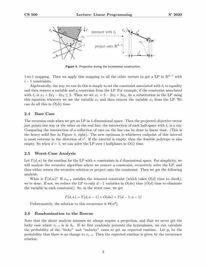
The algorithm is incremental, keeping track of the convex hull of points x1, . . . , xi−1. It addsvertex xi in step i, removing all facets visible from xi and adding in all the new facets induced byxi. See Figure 7.

7


Figure4:Inthefigureonthetop,theshadedregionsarevisiblefacets.Inthefigureonthebottom,visiblefacetsareremovedandnewfacetsareadded.

22-6

Figure 7. Top: Shaded regions are the facets visible from the point X. Bottom: Visible facets are removed and new facetsare added.

4.2 Seidel’s algorithm

First, randomly permutes all the points in P . Then, start out with the convex hull formed by thefirst d points. Let Ci−1 be the convex hull of points p1, . . . pi−1. All ridges in the current hull aremaintained in a search tree, with each ridge having doubly-linked pointers to the two facets formingthat ridge. The search tree for the ridges is height O(d), enabling lookups and insertions in O(d)time. The algorithm adds points xd+1, . . . xn as follows.

1. Find one facet F of Ci−1 that is visible from xi. If there is no visible facet, skip all stepsbelow. A visible facet can be found via linear programming in O(d!i) time as follows. Wewant to find a hyperplane aTx = b (where unknowns are a, b ∈ Rd) such that aTxi = b andeither (1) aTxj ≤ b for all j = 1, . . . , i−1; or (2) aTxj ≥ b for all j = 1, . . . , i−1. This can befound by a linear program in O(d) dimensions, with O(i) constraints. Any solution to this LPwill correspond to a hyperplane supporting a new facet in Ci and a horizon ridge. (Verticesin the facet can be found by finding the d points on the hyperplane in O(di) time; all incidentridges in O(d) time). One of the two facets incident to the horizon ridge is a visible facet.

2. Find all visible facets. Determine all horizon ridges. Delete all visible facets and all visibleridges. Can do this via depth first search since visible facets and invisible facets are separatedby horizon ridges. (Charge deletion time of facets to when they were created.)

3. Construct all new facets. Each horizon ridge corresponds to a new facet combining xi andthe points in the ridge.

8


4. Each new facet contains d ridges. Find each ridge in the ridge search tree, or insert if new.Keep pointers back to appropriate new facets in order to match each ridge to the two facetsthat neighbor it.

4.3 Example for Step 1

The equation (2, 1)T (x, y) = (3, 4) defines a line in R2. In general, aT (x, y) = b defines a line in R2.In Step 1, we want to find a vector a and a vector b to ensure that the point xi is on the line, andthat all other points x1, . . . , xi−1 are on the same side of the halfspace. For example, if i = 3 andx1 = (1, 0), x1 = (0, 1), and x2 = (1, 2), we want to solve the following linear program:

Find variables a1, a2, b1, b2, such that:

(a1, a2)T (1, 2) = (b1, b2)

(a1, a2)T (1, 0) ≤ (b1, b2)

(a1, a2)T (0, 1) ≤ (b1, b2)

Note that technically, each of these lines expands to two linear inequalities. Also, there isnothing to maximize or minimize, we just want to find any feasible point (which is easier than ausual LP). Finally, we also can check feasibility for a LP where the last two lines have ≥ instead of≤.

4.4 Runtime

We assume d is a constant. The time to add point xi is O(i +Ni) where Ni is a random variablegiving the number of new facets created at step i. To see this, first note that step (1) takes O(d!i)time to solve the linear program this is O(i) time assuming d is fixed. In step 2, we delete all visiblefacets and ridges, but the time to do this is charged to when they were created. In step 3, we createNi new facets, taking time O(Ni). In step 4, there are at most O(d ·Ni) new ridges, each of thesecan be processed in the ridge tree in O(d) time, so this step takes O(d2Ni) time. So the total timeto process xi is O(i+Ni).

(Digression: There are d ridges bordering each facet. To see this, note that each facet is uniquelydetermined by d points. And each ridge bordering that facet is uniquely determined by d−1 points.This implies that each facet borders d ridges. For example, if we have the facet v1, v5, v7, v8, v9.Then this facet borders the 5 ridges: (v5, v7, v8, v9); (v1, v7, v8, v9); (v1, v5, v8, v9); (v1, v5, v7, v9);(v1, v5, v7, v8).)

To get the expected runtime, we can compute E(Ni) using the principle of deferred decision(aka backward analysis). Recall our claim that if we have a polytope with i vertices in Rd, then thenumber of facets is O(i⌊d/2⌋). First, we fix one of the O(i⌊d/2⌋) facets of Ci (see Section 5 for how wecan show there are at most O(i⌊d/2⌋) facets). The probability that the i-th point (xi) participatesin this facet is d/i.

Hence using linearity of expectation over allO(i⌊d/2⌋) facets, we can say that E(Ni) = O(di i⌊d/2⌋) =

O(i⌊d/2⌋−1). Thus, the expected runtime of Seidel’s algorithm is:

n#

i=1

O(i+Ni) =

n#

i=1

O(i+ i⌊d/2⌋−1)

= O(n⌊d/2⌋)

9


point p ∈ Rd can be viewed as a d-element vector. (IfO is not the origin, then p can be identified with the vectorp−O.) The polar hyperplane of p, denoted p∗ is defined by

p∗ = x ∈ Rd | (p · x) = 1,

where the expression (p ·x) is just the standard vector dot-product ((p ·x) = p1x1+p2x2+ · · ·+pdxd). Observethat if p is on the unit sphere centered about O, then p∗ is a hyperplane that passes through p and is orthogonalto the vector Op. As we move p away from the origin along this vector, the dual hyperplane moves closer to theorigin, and vice versa, so that the product of their distances from the origin is always 1.Now, let h be any hyperplane that does not contain O. The pole of h, denoted h∗ is the point that satisfies

(h∗ · x) = 1 for all x ∈ h.

1/c

O

O

O

h+

O

h*

p*

O p*+h*

p

ph

Inclusion Reversing

Incidence Preserving

p

c

p*

The Polar Transformation

Fig. 148: The polar transformation and its properties.

Clearly this double transformation is an involution, that is, (p∗)∗ = p and (h∗)∗ = h. The polar transformationpreserves important geometric relationships. Given a hyperplane h, define

h+ = x ∈ Rd | (x · h∗) < 1 h− = x ∈ R

d | (x · h∗) > 1.

That is, h+ is the open halfspace containing the origin and h− is the other open halfspace for h.

Claim: Let p be any point in Rd and let h be any hyperplane in Rd. The polar transformation satisfies thefollowing two properties.Incidence preserving: The polarity transformation preserves incidence relationships between points and

hyerplanes. That is, p belongs to h if and only if h∗ belongs to p∗.Inclusion Reversing: The polarity transformation reverses relative position relationships in the sense that

p belongs to h+ if and only if h∗ belongs to (p∗)+, and p belongs to h− if and only if h∗ belongs to(p∗)−.

In general, any bijective transformation that preserves incidence relations is called a duality. The above claimimplies that polarity is a duality.We can now formalize the aforementioned notion of polytope equivalence. The idea will be to transform apolytope defined as the convex hull of a finite set of points to a polytope defined as the intersection of a finiteset of closed halfspaces. To do this, we need a way of mapping a point to a halfspace. Our approach will be totake the halfspace that contains the origin. For any point p ∈ Rd define the following closed halfspace based onits polar:

p# = p∗+ = x ∈ Rd | (x · p) ≤ 1.

(The notation is ridiculous, but this is easy to parse. First consider the polar hyperplane of p, and take the closedhalfspace containing the origin.) Observe that if a halfspace h+ contains p, then by the inclusion-reversingproperty of polarity, the polar point h∗ is contained within p#.


Figure 8.

Side note: For any value d,&n

i=1 id = O(id+1). This is true since

n#

i=1

id ≤n#

i=1

nd

= nd+1

5 Bounding the Number of Facets

5.1 Polarity

There are two ways to create polytopes: (1) convex hull of a set of points; and (2) intersection ofa collection of closed halfspaces. We show that these are essentially identical through a conceptcaller polar transformation. A polar transformation maps points to hyperplanes and vice versa.This transformation is another example of duality.

Fix any point O in d-dimensional space. O can be the origin, and then we can view any pointp ∈ Rd as a d-element vector. (If O is not the origin then p can be identified with the vector p−O.)Given two vectors p and x, recall that p ·x is the dot-product of p and x. Then the polar hyperplaneof p is denoted :

p∗ = x ∈ Rd, p · x = 1.

Clearly this is linear in the coordinates of x, and so p∗ is a hyperplane in Rd. If p is on theunit sphere centered at O, then p∗ is a hyperplane that passes through p and is orthogonal to the

vector−→Op.

As pmoves away from the origin along this vector, the dual hyperplane move closer to the origin,and vice versa, so that the product of their distances from the origin is always 1. See Figure 8(a).

5.2 Properties

Like with point-line duality, the polar transformation satisfies certain incidence and inclusion prop-erties between points and hyperplanes. For example, let h be any hyperplane that does not containO. The polar point of h, denoted h∗ is the point that satisfies h∗ · x = 1 for all x ∈ h.

Let p be any point in Rd and let h be any hyperplane in Rd. The polar transformation satisfiesthe following properties. For a hyperplane h, let h+ be the halfspace containing the origin and h−

be the otherhalfspace for h. See Figure 8(b).

• Incidence Preserving: Point p belongs to hyperplane h iff h∗ belongs to p∗

10


number of ways, e.g., by translating P so its center of mass coincides with the origin.) By definition,the convex hull is the intersection of the set of all closed halfspaces that contain S. That is, P is theintersection of an infinite set of closed halfspaces. What are these halfspaces? If h+ is a halfspace thatcontains all the points of S, then by the inclusion-reversing property of polarity, the polar point h

is contained within all the hyperplanes p+i , which implies that h 2 P#. This means that, throughpolarity, the halfspaces whose intersection is the convex hull of a set of points is essentially equivalentto the polar points that lie within the polar image of the convex hull. (For example, in Fig. 135(b) thevertices appearing on convex hull of P correspond to the edges of P#, and they appear in the samecyclic order. The redundant point d lies inside of P corresponds to a redundant halfplane d that liesoutside of P#. Observe that every edge of P corresponds to a vertex of P#.)

O

(a) (b)

O

Pa

b c

ef

da

b

c

e

df

P#

Fig. 135: The polar image of a convex hull.

Lemma: Let S = p1, . . . , pn be a set of points in Rd and let P = conv(S). Then its polar image isthe intersection of the corresponding polar halfspaces, that is,

P# =n\

i=1

p+i .

Furthermore:

(i) A point a 2 Rd lies on the boundary of P if and only if the polar hyperplane a supports P#.

(ii) Each k-face of P corresponds to a (d 1 k)-face of P# and given faces f1, f2 of P wheref1 f2, the corresponding faces f#

1 , f#2 of P# satisfy f#

1 f#2 . (That is, inclusion relations

are reversed.)

It is not hard to prove that the polar image of a polytope is an involution, that is (P#)# = P . (SeeBoissonnat and Yvinec for proofs of all these facts.)

Thus, the polar image P# of a polytope is structurally isomorphic to P and all ane relations onP map through polarity to P#. From a computational perspective, this means that we compute thepolar of all the points of P , consider the halfspaces that contain the origin, and take the intersectionof these halfspaces. Thus, the problems of computing convex hulls and computing the intersection ofhalfspaces are computationally equivalent. (In fact, once you have computed the incidence graph forone, you just flip it “upside-down” to get the other!)

Simple and Simplicial Polytopes: Our next objective is to investigate the relationship between the num-ber of vertices and number of facets on a convex polytope. Earlier in the semester we saw that a3-dimensional polyhedron with n vertices has O(n) edges and faces. This was a consequence of Euler’sformula. In order to investigate the generalization of this to higher dimensions, we begin with somedefinitions. A polytope is simplicial if all its proper faces are simplices (see Fig. 136(a)). Observe thatif a polytope is the convex hull of a set of points in general position, then for 0 j d 1, each j-faceis a j-simplex. (For example, in R3 a face with four vertices would imply that these four points arecoplanar, which would violate general position.)


Figure 9.

• Inclusion Reversing: Point p belongs to halfspace h+ iff point h∗ belongs to halfspace(p∗)+. This implies that point p belongs to halfspace h− iff point h∗ belongs to halfspace(p∗)−). Intuitively, this means that the polarity transform reverses relative positions.

Note that a bijective transformation that preserves incidence relations is called a duality. Sothe above claim shows that the polarity transform is another dualtiy.

5.3 Convex Hulls and Halfspace Intersection

We now want to transform a polytope defined as the convex hull of a finite set of points to apolytope defined as the intersection of a finite set of closed halfspaces. To do this, we need amapping from a point to a halfspace. For any point p ∈ Rd, define

p# = (p∗)− = x ∈ Rd | x · p ≤ 1

This just first finds the polar hyperplane of p, and then takes the closed halfspace containing theorigin.

Now for any set of points P ⊆ Rd, define its polar image to be the intersection of these halfspaces.

P# = x ∈ Rd | x · p ≤ 1, ∀p ∈ P

Thus, P# is the intersection of a finite set of closed halfspaces, one for each p ∈ P . Is P#

convex? Yes, since each halfspace is convex, and the intersection of any set of convex spaces isconvex.

The following lemma shows that P and P# are essentially equivalent via polarity.

Lemma 3. Let S = p1, . . . pn be a set of points in Rd and let P = conv(S). Then:

P# = S#

Furthermore:

1. A point a ∈ Rd is on the boundary of P iff the hyperplane a∗ supports P#.

2. Each k-face of P corresponds to a (d− 1− k)-face of P#

Proof: Assume that O is contained within P . We can guarantee this by, e.g., translating P sothat its center of mass coincides with the origin.

11


a

c

b d

3-D polytope: Incidence Graph:

abc acd bcdabd

ab ac ad bc bd

a b c d

cd

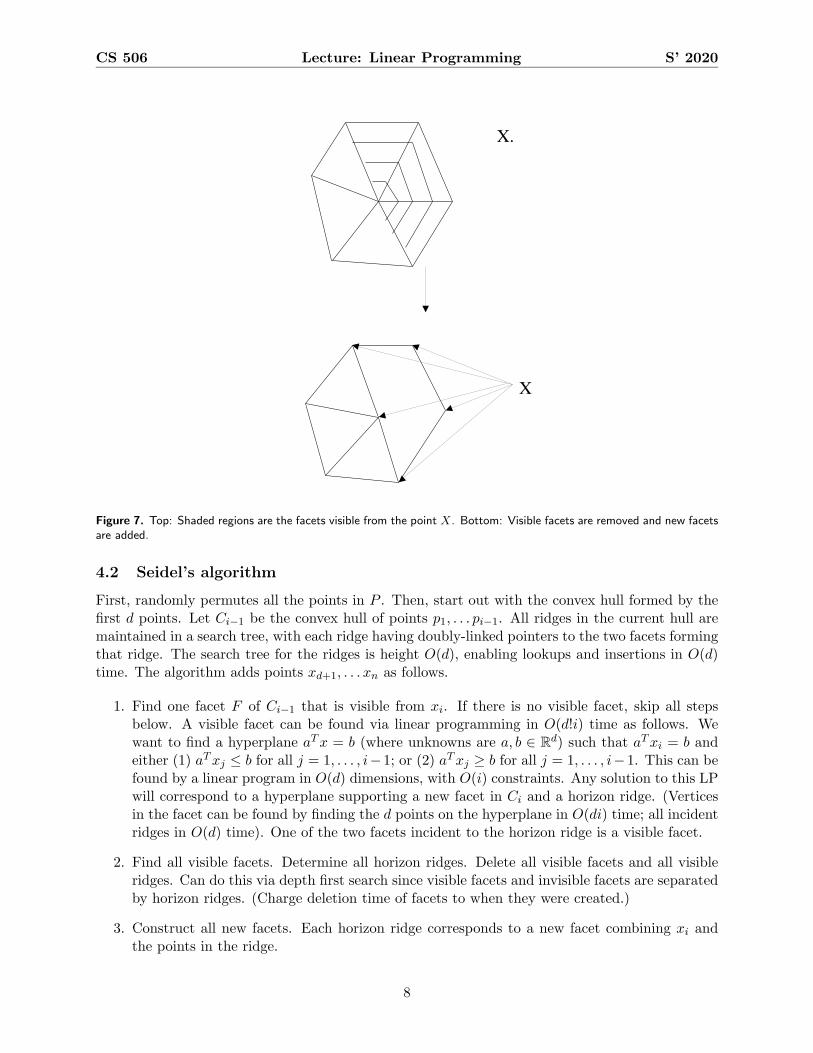
Figure 10. Left: Polytope; Right: Incidence graph for all faces

If we take a dual view, consider a polytope that is the intersection of a set of n halfspaces in general position.Then each j-face is the intersection of exactly (d−j) hyperplanes. A polytope is said to be simple if each j-faceis the intersection of exactly (d−j)-hyperplanes. In particular, this implies that each vertex is incident to exactlyd facets. Further, each j-face can be uniquely identified with a subset of d− j hyperplanes, whose intersectiondefines the face. Following the same logic as in the previous paragraph, it follows that the number of vertices insuch a polytope is naively at most O(nd). (Again, we’ll see later that the tight bound is O(n!d/2").) It followsfrom the results on polarity that a polytope is simple if any only if its polar is simplicial.An important observation about simple polytopes is that the local region around each vertex is equivalent to avertex of a simplex. In particular, if we cut off a vertex of a simple polytope by a hyperplane that is arbitrarilyclose to the vertex, the piece that has been cut off is a d-simplex.It easy to show that among all polytopes having a fixed number of vertices, simplicial polytopes maximize thenumber of faces of all higher degrees. (Observe that otherwise there must be degeneracy among the vertices.Perturbing the points breaks the degeneracy, and will generally split faces of higher degree into multiple facesof lower degree.) Dually, among all polytopes having a fixed number of facets, simple polytopes maximize thenumber of faces of all lower degrees.Another observation allows us to provide crude bounds on the number of faces of various dimensions. Considerfirst a simplicial polytope having n vertices. Each (j − 1)-face can be uniquely identified with a subset of jpoints whose convex hull gives this face. Of course, unless the polytope is a simplex, not all of these subsets willgive rise to a face. Nonetheless this yields the following naive upper bound on the numbers of faces of variousdimensions. By applying the polar transformation we in fact get two bounds, one for simplicial polytopes andone for simple polytopes.

Simplicial Polytope Simple Polytope

Fig. 150: Simplicial and simple polytopes.

Lemma: (Naive bounds)(i) The number faces of dimension j of a polytope with n vertices is at most

( nj+1

)

.(ii) The number of faces of dimension j of a polytope with n facets is at most

( nd−j

)

.

These naive bounds are not tight. Tight bounds can be derived using more sophisticated relations on the numbersof faces of various dimensions, called the Dehn-Sommerville relations. We will not cover these, but see thediscussion below of the Upper Bound Theorem.

The Combinatorics of Polytopes: Let P be a d-polytope. For −1 ≤ k ≤ d, let nk(P ) denote the number of k-facesof P . Clearly n−1(P ) = nd(P ) = 1. The numbers of faces of other dimensions generally satisfy a number ofcombinatorial relationships. The simplest of these is called Euler’s relation:

Theorem: (Euler’s Relation) Given any d-polytope P we have∑d

k=−1(−1)knk(P ) = 0.

This says that the alternating sum of the numbers of faces sums to 0. For example, a cube has 8 vertices, 12edges, 6 facets, and together with the faces of dimension −1 and d we have

−1 + 8− 12 + 6− 1 = 0.


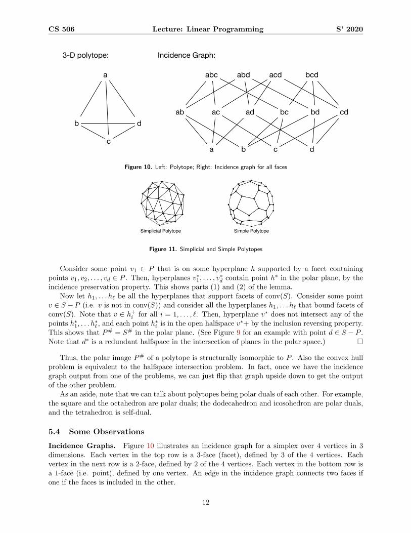
Figure 11. Simplicial and Simple Polytopes

Consider some point v1 ∈ P that is on some hyperplane h supported by a facet containingpoints v1, v2, . . . , vd ∈ P . Then, hyperplanes v∗1, . . . , v

∗d contain point h∗ in the polar plane, by the

incidence preservation property. This shows parts (1) and (2) of the lemma.Now let h1, . . . hℓ be all the hyperplanes that support facets of conv(S). Consider some point

v ∈ S −P (i.e. v is not in conv(S)) and consider all the hyperplanes h1, . . . hℓ that bound facets ofconv(S). Note that v ∈ h+i for all i = 1, . . . , ℓ. Then, hyperplane v∗ does not intersect any of thepoints h∗1, . . . h

∗ℓ , and each point h∗i is in the open halfspace v∗+ by the inclusion reversing property.

This shows that P# = S# in the polar plane. (See Figure 9 for an example with point d ∈ S − P .Note that d∗ is a redundant halfspace in the intersection of planes in the polar space.)

Thus, the polar image P# of a polytope is structurally isomorphic to P . Also the convex hullproblem is equivalent to the halfspace intersection problem. In fact, once we have the incidencegraph output from one of the problems, we can just flip that graph upside down to get the outputof the other problem.

As an aside, note that we can talk about polytopes being polar duals of each other. For example,the square and the octahedron are polar duals; the dodecahedron and icosohedron are polar duals,and the tetrahedron is self-dual.

5.4 Some Observations

Incidence Graphs. Figure 10 illustrates an incidence graph for a simplex over 4 vertices in 3dimensions. Each vertex in the top row is a 3-face (facet), defined by 3 of the 4 vertices. Eachvertex in the next row is a 2-face, defined by 2 of the 4 vertices. Each vertex in the bottom row isa 1-face (i.e. point), defined by one vertex. An edge in the incidence graph connects two faces ifone if the faces is included in the other.

12


v

This 3-face is charged by vxd

Fig. 137: Proof of the Upper Bound Theorem in R5. In this case the three edges above v span a 3-face whoselowest vertex is v.

number of (dj)-element subsets of hyerplanes.) Summing this up over all the faces of dimensiondd/2e and higher we find that the number of vertices is at most

2dX

j=dd/2e

n

d j

.

By changing the summation index to k = d j and making the observation thatnk

is O(nk), we

have that the number of vertices is at most

2

bd/2cX

k=0

n

k

=

bd/2cX

k=0

O(nk).

This is a geometric series, and so is dominated asymptotically by its largest term. Therefore itfollows that the number of charges, that is, the number of vertices is at most

Onbd/2c

,

and this completes the proof.

Is this bound tight? Yes it is. There is a family of polytopes, called cyclic polytopes, which match thisasymptotic bound. (See Boissonnat and Yvinec for a definition and proof.)

Lecture 25: Kirkpatrick’s Planar Point Location

Point Location: In point location we are given a polygonal subdivision (formally, a cell complex). Theobjective is to preprocess this subdivision into a data structure so that given a query point q, we caneciently determine which face of the subdivision contains q. We may assume that each face has someidentifying label, which is to be returned. We also assume that the subdivision is represented in any“reasonable” form (e.g., as a DCEL). In general q may coincide with an edge or vertex. To simplifymatters, we will assume that q does not lie on an edge or vertex, but these special cases are not hardto handle.

It is remarkable that although this seems like such a simple and natural problem, it took quite a longtime to discover a method that is optimal with respect to both query time and space. Let n denotethe number of vertices of the subdivision. By Euler’s formula, the number of edges and faces are O(n).It has long been known that there are data structures that can perform these searches reasonably well(e.g. quad-trees and kd-trees), but for which no good theoretical bounds could be proved. There were


Figure 12.

Two observations. First, the incidence graph of the simplex in the polar plane, can be readbottom up by just taking the polar halfplane v∗ for each vertex v in the incidence graph, andthinking of each face as the intersection of a collection of these halfplanes. Second, for a simplex,there are exactly d + 1 facets. But for a arbitrary polytope, that is the convex hull of n points,there may be many more facets.

Simple and Simplicial Polytopes. If a polytope is the convex hull of a set of points in Rd ingeneral position, then for all 0 ≤ j ≤ d − 1, each j-face is a j-simplex. Such a polytope is calledsimplicial (see Figure 11.)

In the dual view, consider a polytope that is the intersection of n halfspaces in general position.Each j-face for 0 ≤ j ≤ d − 1 is the intersection of exactly d − j hyperplanes. Such a polytope issaid to be simple. Note that in simple polytopes, each vertex is incident to exactly d facets. Thus,the local region around any vertex is equivalent to a simplex.

Among all polytopes with a fixed number of vertices, simplicial polytopes maximize the numberof facets. To see this, note that if there is a degeneracy (i.e. d+1 points on one facet), perturbingsome point on this facet will break it into multiple facets. Dually, among all polytopes with a fixednumber of facets, simple polytopes maximize the number of vertices.

5.5 How Many Facets?

So, how many facets are in a convex hull defined by n points in d dimensional space? The followingtheorem has a remarkably beautiful proof (also due to Seidel) that uses polar duality.

Theorem 1. A polytope in Rd that is the convex hull of n points has O(n⌊d/2⌋) facets. A polytopein Rd that is the intersection of n halfspaces has O(n⌊d/2⌋) vertices.

Proof: We will prove the polar form of the theorem. Consider a polytope defined by intersectionof n halfspaces in general position. By the discussion in the last section, this gives rise to asimple polytope, which maximizes the number of vertices. Suppose by convention that xd is thevertical axis. Then given a face, its highest and lowest vertices are defined as those having themaximum and minimum xd coordinates, respectively. (Note that there are no ties, assumingsymbolic perturbation). Our proof is based on a charging argument. We place a charge at eachvertex. We then move the charge at each vertex to a specially chosen incident face so that no facereceives more than 2 charges.

Consider some vertex v. Note that there are d edges (1-faces) that are incident to v (SeeFigure 12 for example in R5). Consider a horizontal (i.e. orthogonal to xd) hyperplane that passes

13


through v. Note that at least ⌈d/2⌉ of the edges must lie on the same side of this hyperplane (again,use symbolic perturbation to ensure no two points have exactly the same xd coordinate, so none ofthese edges lie on this hyperplane).

Hence, there is a face of dimension at least ⌈d/2⌉ that spans these edges and is incident to v(i.e. the 3-face above v in Figure 12). So v is either the highest or lowest vertex on this face. Weassign v’s charge to this face. Thus, we charge every vertex to a face of dimension at least ⌈d/2⌉,and every such face will be charged twice.

So how many charges are there in total? The number of j faces is'

nd−j

(, since each j face is the

intersection of d− j halfspaces. Thus, the total number of charges is:

2

d−1#

j=⌈d/2⌉

)n

d− j

*= 2

⌊d/2⌋#

i=1

)n

i

*

≤ 2

⌊d/2⌋#

i=1

ni

= O(n⌊d/2⌋)

Note the second step holds since'nx

(≤ nx. True since

'nx

(is the number of ways to choose x

items from a set of size n without replacement, and nx is the number of ways to choose x itemsfrom a set of n with replacement.

The last step holds since

S =

ℓ#

i=1

bi

implies that

bS =

ℓ+1#

i=2

bi

Subtracting the top equation from the bottom, we get that S− bS = b− bℓ+1. This implies that

S = b−bℓ+1

1−b = bℓ+1−bb−1 = b(bℓ−1)

b−1 = O(bℓ)

Is this bound tight? Yes. There is a family of polytopes called cyclic polytopes which matchthis asymptotic bound.

References

[1] David Mount. Computational Geometry. http://www.cs.umd.edu/class/fall2016/cmsc754/Lects/cmsc754-fall16-lects.pdf, 2016.

14

http://www.cs.umd.edu/class/fall2016/cmsc754/Lects/cmsc754-fall16-lects.pdf

Lecture 8: Linear Programming

Documents

Transcript of Lecture 8: Linear Programming