Lecture 8 Inferences about Population Variance. Goodness ...

Lecture 8. Inferences about population variance. Goodness of fit and independence

BIOSTATISTICS

4-04-2020

dr. Petr Nazarov

[email protected]

Lecture 8

Inferences about Population Variance.

Goodness of Fit and Independence

Multiomics Data Science

Lecture 8. Inferences about population variance. Goodness of fit and independence 2

OUTLINELecture 8

PART I

Interval estimation for population variance

variance sampling distribution, 2 statistics

calculation of interval estimation

hypothesis tests for a population variance

Comparison of variances of two populations

F-statistics

formulation of hypotheses and testing

PART II

2 criterion of goodness of fit

multinomial distribution

continuous distributions

Independence


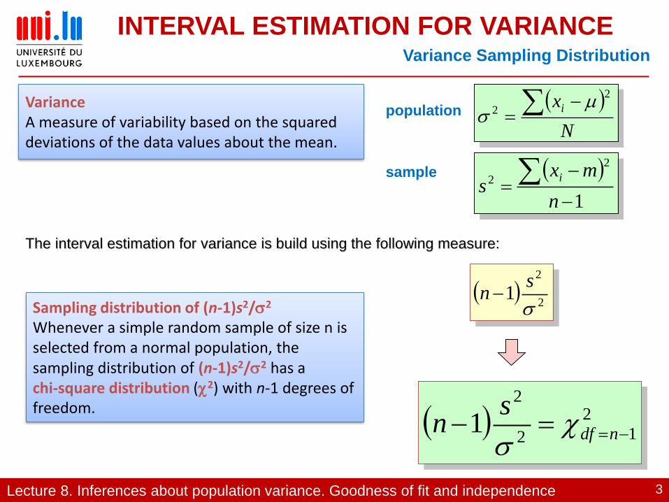
INTERVAL ESTIMATION FOR VARIANCEVariance Sampling Distribution

Sampling distribution of (n-1)s2/2

Whenever a simple random sample of size n is selected from a normal population, the sampling distribution of (n-1)s2/2 has achi-square distribution (2) with n-1 degrees of freedom.

VarianceA measure of variability based on the squared deviations of the data values about the mean.

N

xi

2

2

1

2

2

n

mxs

isample

population

The interval estimation for variance is build using the following measure:

2

2

1

sn

2

12

2

1 ndf

sn


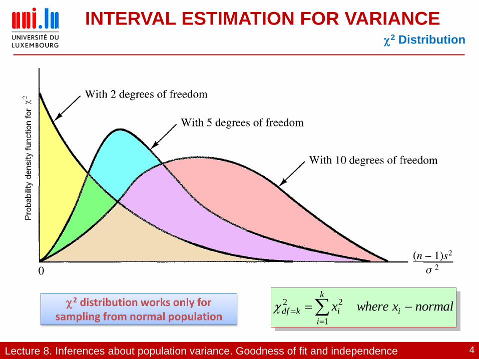
INTERVAL ESTIMATION FOR VARIANCE2 Distribution

2 distribution works only for sampling from normal population

normalxwherex i

k

i

ikdf

1

22


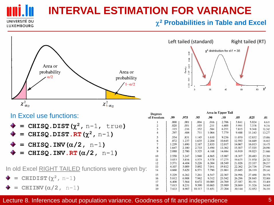
INTERVAL ESTIMATION FOR VARIANCE2 Probabilities in Table and Excel

In Excel use functions:

= CHISQ.DIST(2, n-1, true)

= CHISQ.DIST.RT(2, n-1)

= CHISQ.INV(/2, n-1)

= CHISQ.INV.RT(/2, n-1)

In old Excel RIGHT TAILED functions were given by:

= CHIDIST(2, n-1)

= CHIINV(/2, n-1)

Right tailed (RT)Left tailed (standard)


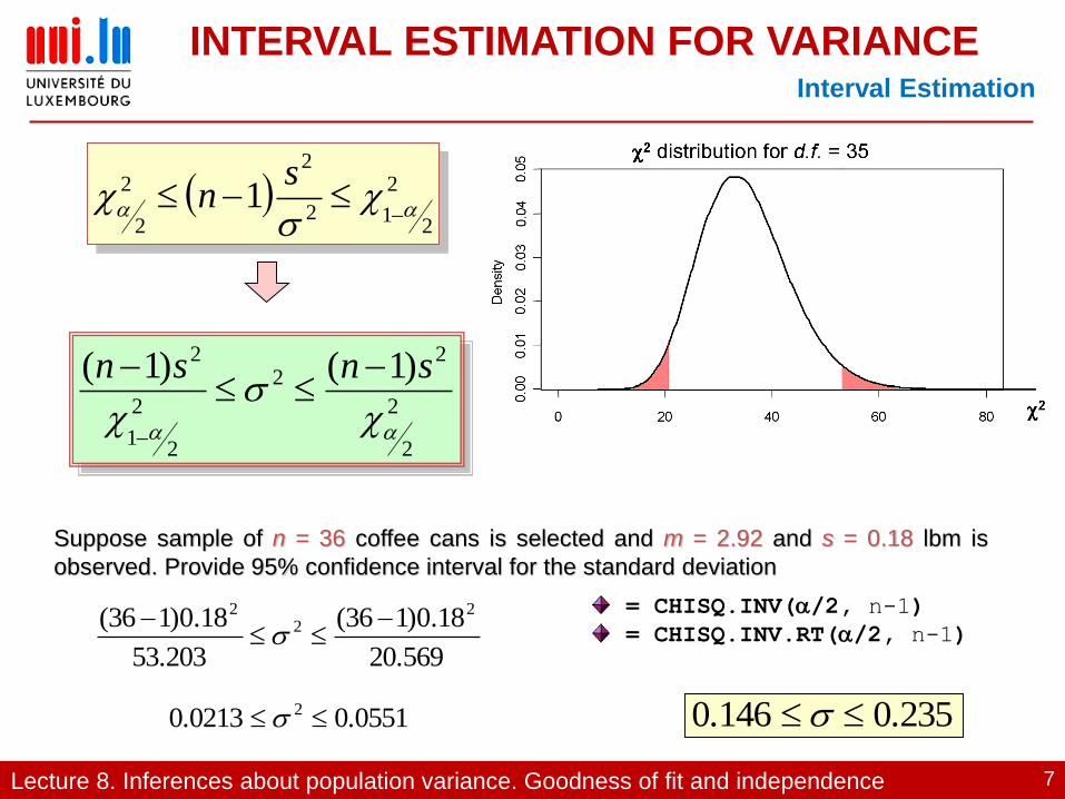
INTERVAL ESTIMATION FOR VARIANCE2 Distribution for Interval Estimation

2

22 1

sn

2 distribution for d.f. = 19


INTERVAL ESTIMATION FOR VARIANCEInterval Estimation

2

212

22

2

1

s

n

2

2

22

2

21

2 )1()1(

snsn

Suppose sample of n = 36 coffee cans is selected and m = 2.92 and s = 0.18 lbm is

observed. Provide 95% confidence interval for the standard deviation

20.569

18.0)136(

53.203

18.0)136( 22

2

0.2350.146 0.05510.0213 2

= CHISQ.INV(/2, n-1)

= CHISQ.INV.RT(/2, n-1)


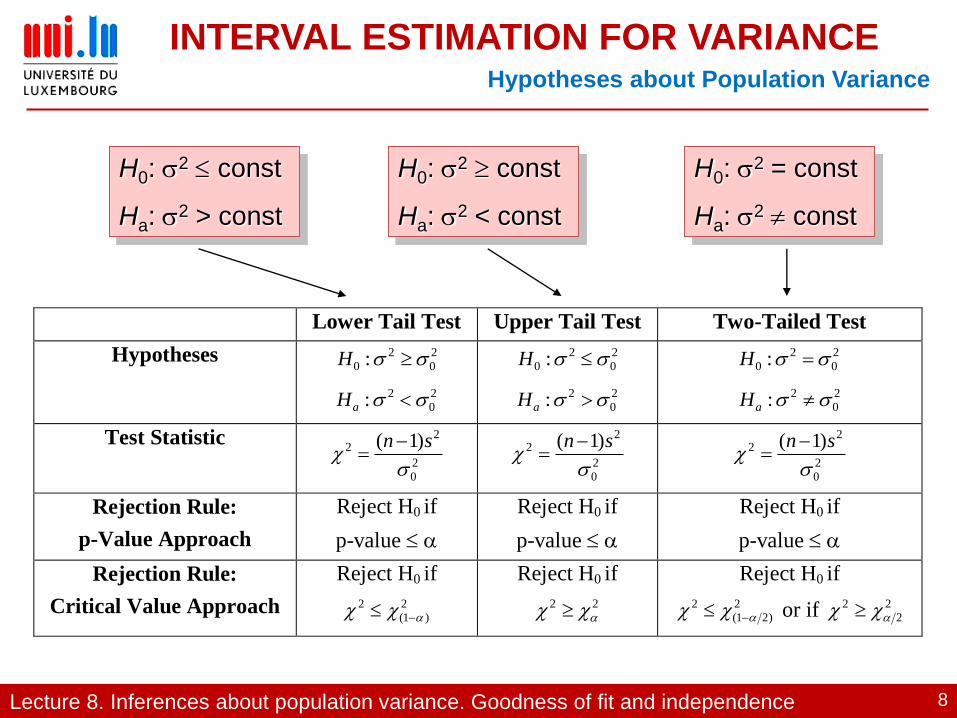
INTERVAL ESTIMATION FOR VARIANCEHypotheses about Population Variance

H0: 2 const

Ha: 2 > const

H0: 2 const

Ha: 2 < const

H0: 2 = const

Ha: 2 const

Lower Tail Test Upper Tail Test Two-Tailed Test

Hypotheses 2

0

2

0 : H

2

0

2: aH

2

0

2

0 : H

2

0

2: aH

2

0

2

0 : H

2

0

2: aH

Test Statistic 2

0

22 )1(

sn

2

0

22 )1(

sn

2

0

22 )1(

sn

Rejection Rule:

p-Value Approach

Reject H0 if

p-value

Reject H0 if

p-value

Reject H0 if

p-value

Rejection Rule:

Critical Value Approach

Reject H0 if

2

)1(

2

Reject H0 if

22

Reject H0 if

2

)21(

2

or if 2

2

2


VARIANCES OF TWO POPULATIONSSampling Distribution

In many statistical applications we need a comparison between variances of two

populations. In fact well-known ANOVA-method is base on this comparison.

The statistics is build for the following measure:22

21

s

sF

Sampling distribution of s12/s2

2 when 12= 2

2

Whenever a independent simple random samples of size n1 and n2 are selected from two normal populations with equal variances, the sampling of s1

2/s22 has F-distribution

with n1-1 degree of freedom for numerator and n2-1 for denominator.

F-distribution for 20 d.f. in numerator and 20 d.f. in denominator

In Excel use functions:

= F.TEST(data1,data2)


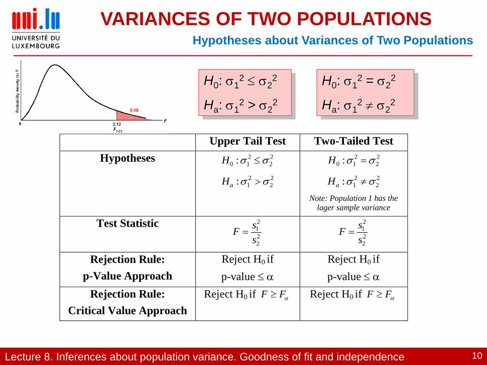
VARIANCES OF TWO POPULATIONSHypotheses about Variances of Two Populations

H0: 12 2

2

Ha: 12 > 2

2

H0: 12 = 2

2

Ha: 12 2

2

Upper Tail Test Two-Tailed Test

Hypotheses 2

2

2

10 : H

2

2

2

1: aH

2

2

2

10 : H

2

2

2

1: aH

Note: Population 1 has the lager sample variance

Test Statistic 2

2

2

1

s

sF

2

2

2

1

s

sF

Rejection Rule:

p-Value Approach

Reject H0 if

p-value

Reject H0 if

p-value

Rejection Rule:

Critical Value Approach

Reject H0 if FF Reject H0 if FF


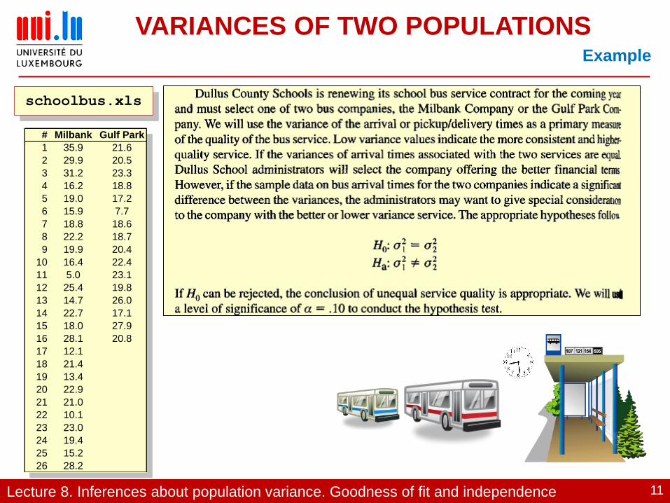
VARIANCES OF TWO POPULATIONSExample

schoolbus.xls

# Milbank Gulf Park

1 35.9 21.6

2 29.9 20.5

3 31.2 23.3

4 16.2 18.8

5 19.0 17.2

6 15.9 7.7

7 18.8 18.6

8 22.2 18.7

9 19.9 20.4

10 16.4 22.4

11 5.0 23.1

12 25.4 19.8

13 14.7 26.0

14 22.7 17.1

15 18.0 27.9

16 28.1 20.8

17 12.1

18 21.4

19 13.4

20 22.9

21 21.0

22 10.1

23 23.0

24 19.4

25 15.2

26 28.2


VARIANCES OF TWO POPULATIONSExample

schoolbus.xls

# Milbank Gulf Park

1 35.9 21.6

2 29.9 20.5

3 31.2 23.3

4 16.2 18.8

5 19.0 17.2

6 15.9 7.7

7 18.8 18.6

8 22.2 18.7

9 19.9 20.4

10 16.4 22.4

11 5.0 23.1

12 25.4 19.8

13 14.7 26.0

14 22.7 17.1

15 18.0 27.9

16 28.1 20.8

17 12.1

18 21.4

19 13.4

20 22.9

21 21.0

22 10.1

23 23.0

24 19.4

25 15.2

26 28.2

1. Let us start from estimation of the variances for 2 data sets

Milbank: s12 = 48

Gulf Park: s22 = 20

Milbank: 12 48 (29.5 91.5)

Gulf Park: 22 20 (10.9 47.9)

interval estimation (optionally)

2. Let us calculate the F-statistics

40.220

4822

21

s

sF

3. … and p-value = 0.08

In Excel use one of the functions:

= 2*F.DIST.RT(F,n1-1,n2-1)

= F.TEST(data1,data2)

p-value = 0.08 < = 0.1


Goodness of Fit and

Independence


TEST OF GOODNESS OF FITMultinomial Population

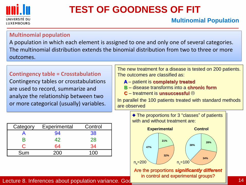
Multinomial population A population in which each element is assigned to one and only one of several categories. The multinomial distribution extends the binomial distribution from two to three or more outcomes.

The proportions for 3 “classes” of patients

with and without treatment are:

Experimental Control

ne=200 nc=100

Are the proportions significantly different

in control and experimental groups?

The proportions for 3 The proportions for 3 ““classesclasses”” of patients of patients

with and without treatment are:with and without treatment are:

Experimental ControlExperimental Control

nnee=200 =200 nncc=100 =100

Are the proportions Are the proportions significantly differentsignificantly different

in control and experimental groups? in control and experimental groups?

21%

32%

47%

21%

32%

47%38%

34%

28%38%

34%

28%




ne=200 nc=100






nnee=200 =200 nncc=100 =100



21%

32%

47%

21%

32%

47%38%

34%

28%38%

34%

28%

The new treatment for a disease is tested on 200 patients.

The outcomes are classified as:

A – patient is completely treated

B – disease transforms into a chronic form

C – treatment is unsuccessful

In parallel the 100 patients treated with standard methods

are observed

Contingency table = CrosstabulationContingency tables or crosstabulations are used to record, summarize and analyze the relationship between two or more categorical (usually) variables.

Category Experimental Control

A 94 38

B 42 28

C 64 34

Sum 200 100


TEST OF GOODNESS OF FITGoodness of Fit




ne=200 nc=100






nnee=200 =200 nncc=100 =100



21%

32%

47%

21%

32%

47%38%

34%

28%38%

34%

28%




ne=200 nc=100






nnee=200 =200 nncc=100 =100



21%

32%

47%

21%

32%

47%38%

34%

28%38%

34%

28%

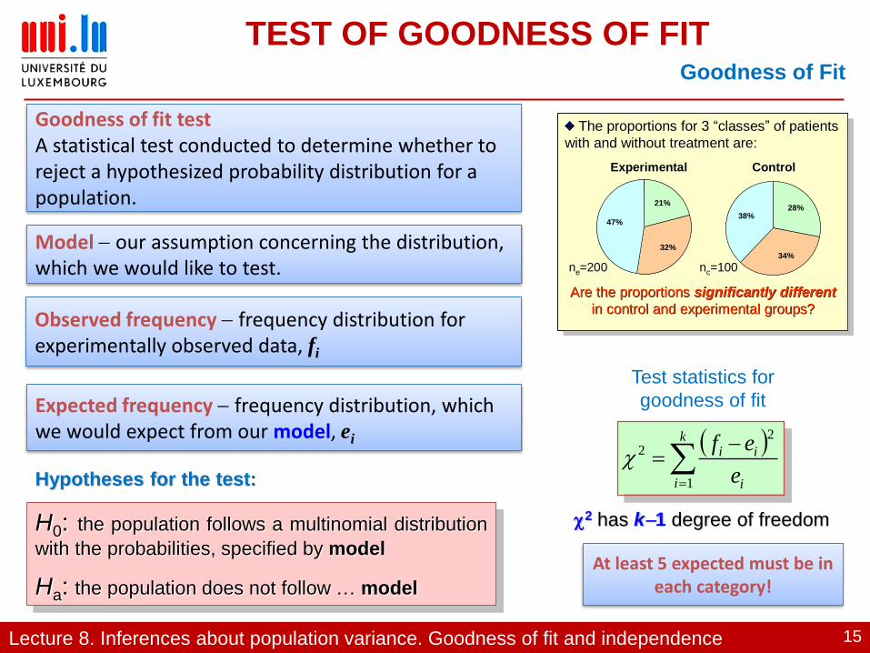
Goodness of fit test A statistical test conducted to determine whether to reject a hypothesized probability distribution for a population.

Model our assumption concerning the distribution, which we would like to test.

Observed frequency frequency distribution for experimentally observed data, fi

Expected frequency frequency distribution, which we would expect from our model, ei

k

i i

ii

e

ef

1

2

2

Test statistics for

goodness of fit

2 has k1 degree of freedom

Hypotheses for the test:

H0: the population follows a multinomial distribution

with the probabilities, specified by model

Ha: the population does not follow … model

At least 5 expected must be in each category!


TEST OF GOODNESS OF FITExample

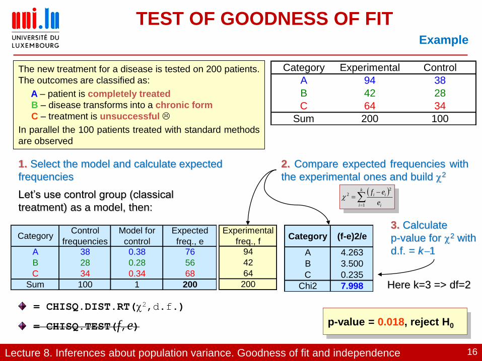
The new treatment for a disease is tested on 200 patients.

The outcomes are classified as:

A – patient is completely treated

B – disease transforms into a chronic form

C – treatment is unsuccessful

In parallel the 100 patients treated with standard methods

are observed

1. Select the model and calculate expected

frequencies

Let’s use control group (classical

treatment) as a model, then:

3. Calculate

p-value for 2 with

d.f. = k1

= CHISQ.DIST.RT(2,d.f.)

= CHISQ.TEST(f,e) p-value = 0.018, reject H0

2. Compare expected frequencies with

the experimental ones and build 2

k

i i

ii

e

ef

1

2

2

CategoryControl

frequencies

Model for

control

Expected

freq., e

A 38 0.38 76

B 28 0.28 56

C 34 0.34 68

Sum 100 1 200

Experimental

freq., f

94

42

64

200

Category (f-e)2/e

A 4.263

B 3.500

C 0.235

Chi2 7.998

Category Experimental Control

A 94 38

B 42 28

C 64 34

Sum 200 100

Here k=3 => df=2


TEST OF INDEPENDENCEGoodness of Fit for Independence Test: Example

Alber's Brewery manufactures and distributes three types of beer: white, regular, and

dark. In an analysis of the market segments for the three beers, the firm's market

research group raised the question of whether preferences for the three beers differ

among male and female beer drinkers. If beer preference is independent of the gender

of the beer drinker, one advertising campaign will be initiated for all of Alber's beers.

However, if beer preference depends on the gender of the beer drinker, the firm will tailor

its promotions to different target markets.

H0: Beer preference is independent of

the gender of the beer drinker

Ha: Beer preference is not independent

of the gender of the beer drinker

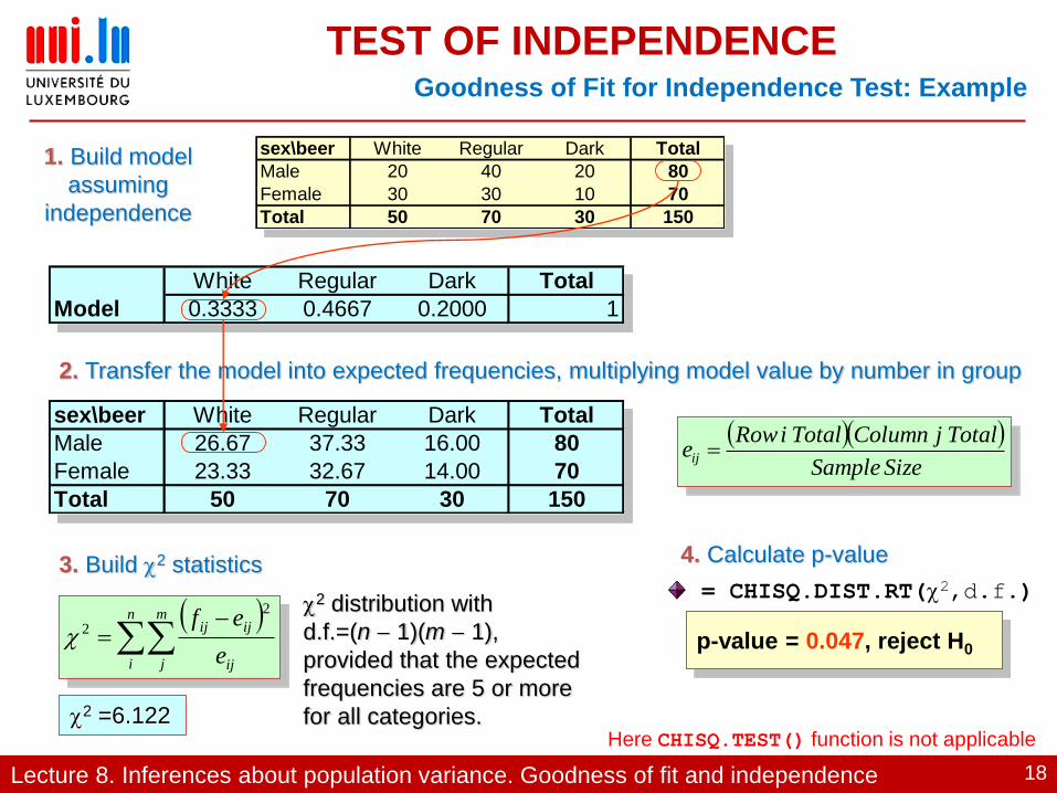
sex\beer White Regular Dark Total

Male 20 40 20 80

Female 30 30 10 70

Total 50 70 30 150

beer.xls


TEST OF INDEPENDENCEGoodness of Fit for Independence Test: Example

White Regular Dark Total

Model 0.3333 0.4667 0.2000 1


Male 20 40 20 80

Female 30 30 10 70

Total 50 70 30 150

1. Build model

assuming

independence

2. Transfer the model into expected frequencies, multiplying model value by number in group


Male 26.67 37.33 16.00 80

Female 23.33 32.67 14.00 70

Total 50 70 30 150

SizeSample

TotaljColumnTotaliRoweij

n

i

m

j ij

ijij

e

ef2

2

3. Build 2 statistics

2 distribution with

d.f.=(n 1)(m 1),

provided that the expected

frequencies are 5 or more

for all categories.2 =6.122

4. Calculate p-value

p-value = 0.047, reject H0

= CHISQ.DIST.RT(2,d.f.)

Here CHISQ.TEST() function is not applicable


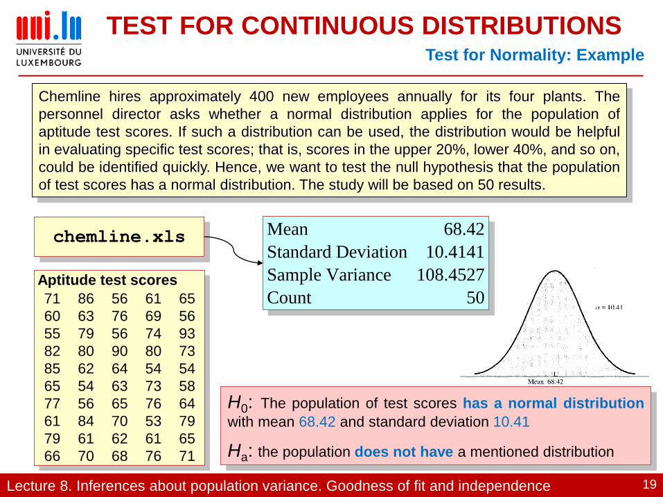
TEST FOR CONTINUOUS DISTRIBUTIONSTest for Normality: Example

Chemline hires approximately 400 new employees annually for its four plants. The

personnel director asks whether a normal distribution applies for the population of

aptitude test scores. If such a distribution can be used, the distribution would be helpful

in evaluating specific test scores; that is, scores in the upper 20%, lower 40%, and so on,

could be identified quickly. Hence, we want to test the null hypothesis that the population

of test scores has a normal distribution. The study will be based on 50 results.

Aptitude test scores

71 86 56 61 65

60 63 76 69 56

55 79 56 74 93

82 80 90 80 73

85 62 64 54 54

65 54 63 73 58

77 56 65 76 64

61 84 70 53 79

79 61 62 61 65

66 70 68 76 71

chemline.xls

H0: The population of test scores has a normal distribution

with mean 68.42 and standard deviation 10.41

Ha: the population does not have a mentioned distribution

Mean 68.42

Standard Deviation 10.4141

Sample Variance 108.4527

Count 50


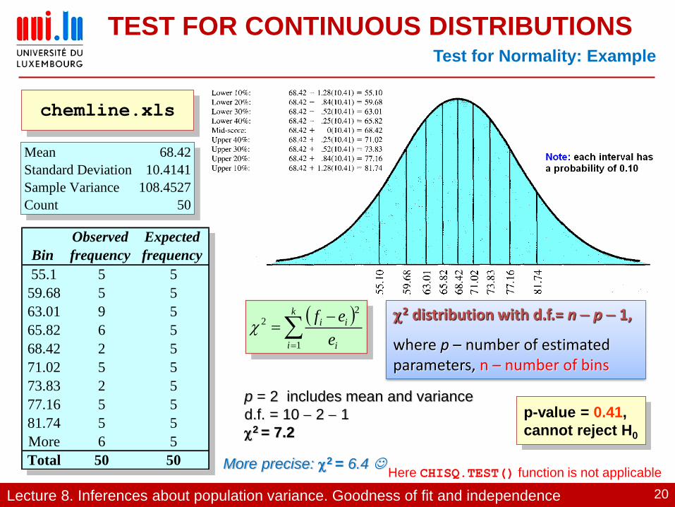
TEST FOR CONTINUOUS DISTRIBUTIONSTest for Normality: Example

chemline.xls

Mean 68.42

Standard Deviation 10.4141

Sample Variance 108.4527

Count 50

Bin

Observed

frequency

Expected

frequency

55.1 5 5

59.68 5 5

63.01 9 5

65.82 6 5

68.42 2 5

71.02 5 5

73.83 2 5

77.16 5 5

81.74 5 5

More 6 5

Total 50 50

k

i i

ii

e

ef

1

2

22 distribution with d.f.= n p 1,

where p – number of estimated parameters, n – number of bins

p = 2 includes mean and variance

d.f. = 10 2 1

2 = 7.2

p-value = 0.41,

cannot reject H0

Here CHISQ.TEST() function is not applicableMore precise: 2 = 6.4


Thank you for your

attention

QUESTIONS ?

Lecture 8 Inferences about Population Variance. Goodness ...

Documents

Transcript of Lecture 8 Inferences about Population Variance. Goodness ...