Lecture 7: Signal Transduction - Ed
33
1 computational systems biology Lecture 8: Signal Transduction Computational Systems Biology Images from: D. L. Nelson, Lehninger Principles of Biochemistry, IV Edition – Chapter 12 E. Klipp, Systems Biology in Practice, Wiley-VCH, 2005 – Chapter 6
Transcript of Lecture 7: Signal Transduction - Ed
1
computational systems biology
Lecture 8: Signal Transduction
Computational Systems Biology
Images from: D. L. Nelson, Lehninger Principles of Biochemistry, IV Edition – Chapter 12E. Klipp, Systems Biology in Practice, Wiley-VCH, 2005 – Chapter 6
computational systems biology
2
Summary:
• Introduction on cell signalling– Metabolism vs. Signal transduction
• The signalling paradigm and some typical components:– The receptor– G protein– MAP kinase cascade

computational systems biology
3
Cell Signalling
computational systems biology
4
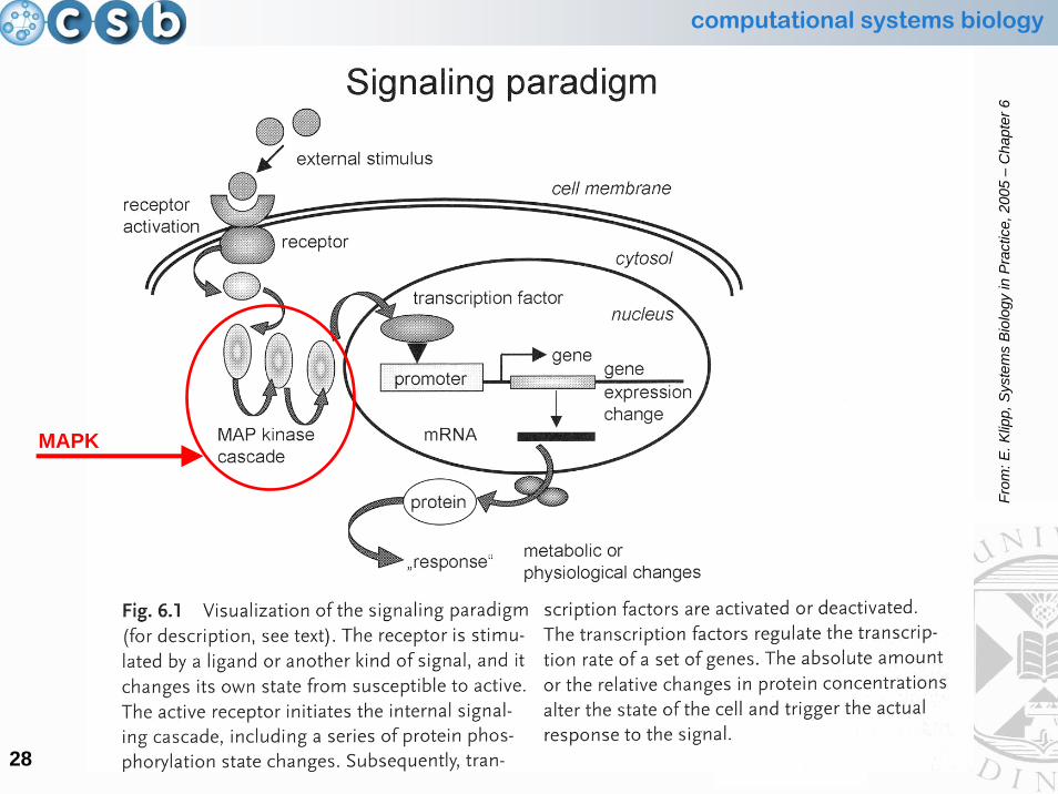
Signal Transduction
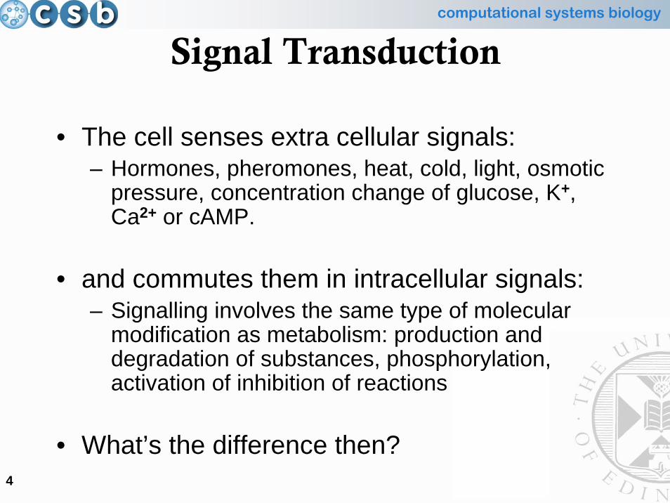
• The cell senses extra cellular signals:– Hormones, pheromones, heat, cold, light, osmotic
pressure, concentration change of glucose, K+, Ca2+ or cAMP.
• and commutes them in intracellular signals:– Signalling involves the same type of molecular
modification as metabolism: production and degradation of substances, phosphorylation, activation of inhibition of reactions
• What’s the difference then?

computational systems biology
5
Metabolism vs. Signal Transduction
Metabolism
• Provides mass transfer
• Quantity of converted material: μM or mM
• A metabolic network is determined by the present set of enzymes
• The catalyst to substrate ratio is low (quasi-steady-state assumption in Michaelis-Menten kinetics)
Signal Transduction
• Provides information transfer
• Quantities: 10 to 104
molecules per cell
• A signal pathway may assemble dynamically
• Amount of catalyst and substrate in the same order of magnitude
computational systems biology
6
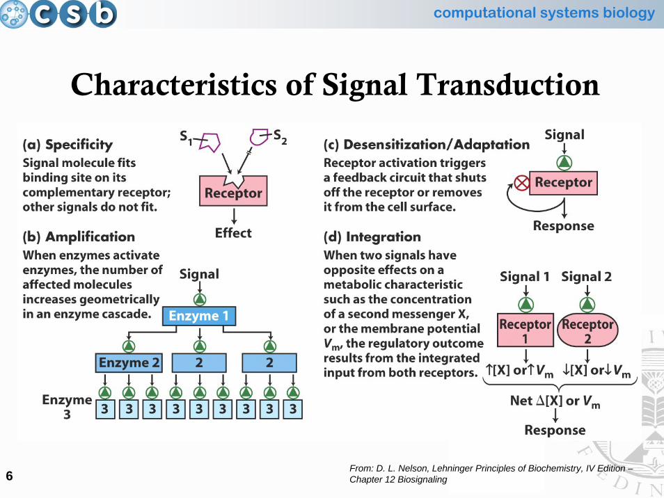
Characteristics of Signal Transduction
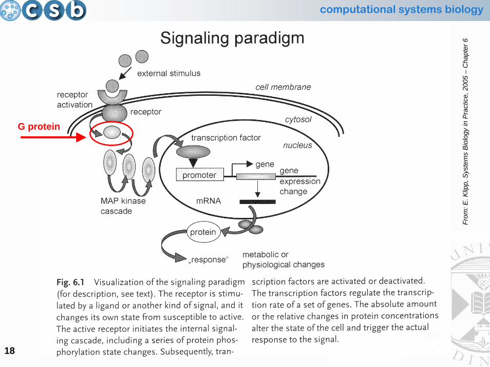
From: D. L. Nelson, Lehninger Principles of Biochemistry, IV Edition –Chapter 12 Biosignaling
computational systems biology
7
Signalling Paradigm:the Receptor
computational systems biology
8
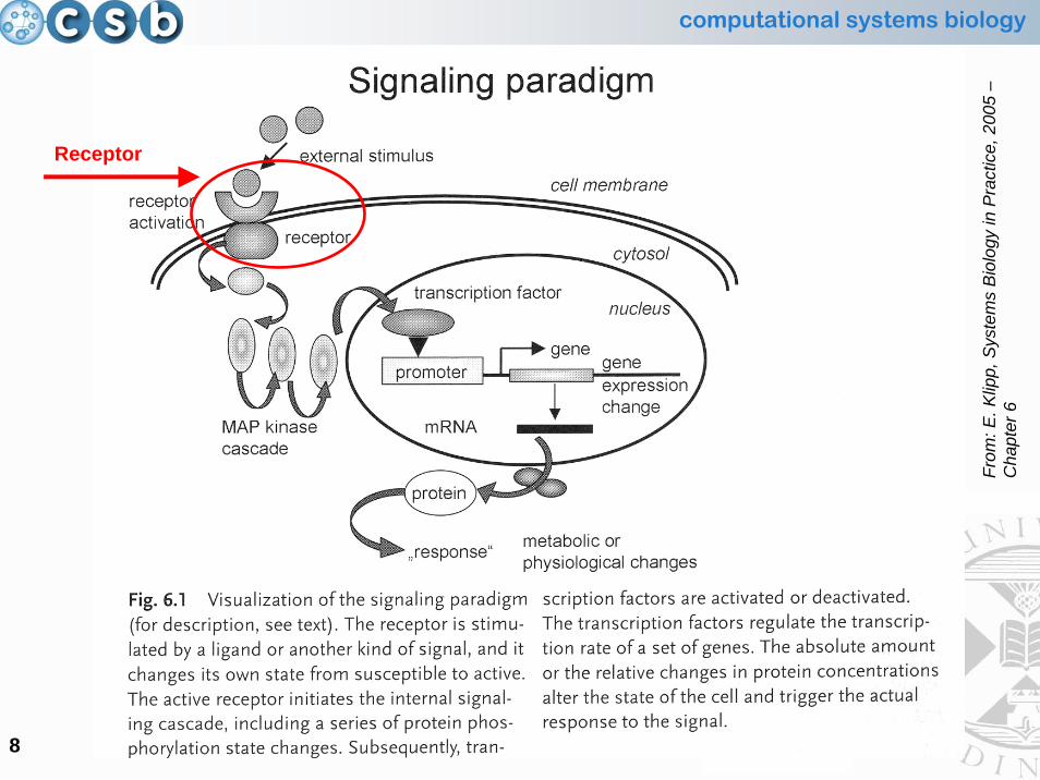
Receptor
From
: E. K
lipp,
Sys
tem
s B
iolo
gy in
Pra
ctic
e, 2
005
–C
hapt
er 6
computational systems biology
9
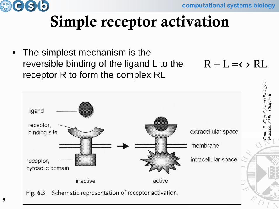
Simple receptor activation
• The simplest mechanism is the reversible binding of the ligand L to the receptor R to form the complex RL
RLLR =↔+
From
: E. K
lipp,
Sys
tem
s B
iolo
gy in
P
ract
ice,
200
5 –
Cha
pter
6
computational systems biology
10
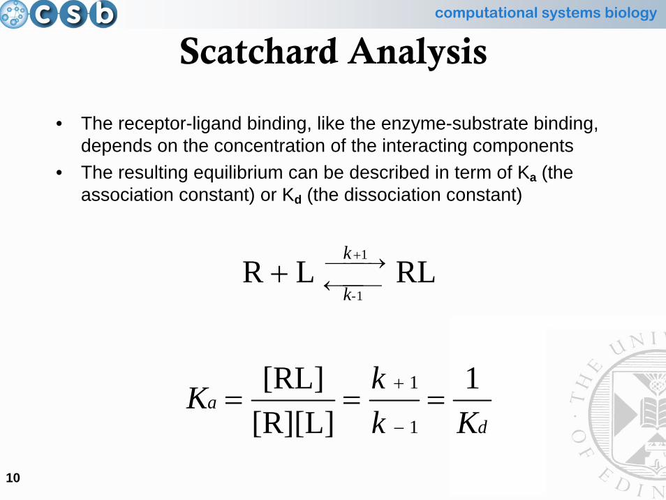
Scatchard Analysis
• The receptor-ligand binding, like the enzyme-substrate binding, depends on the concentration of the interacting components
• The resulting equilibrium can be described in term of Ka (the association constant) or Kd (the dissociation constant)
da
k
k
KkkK
-
1[R][L][RL]
RL LR
1
1
1
1
===
+
−
+
⎯⎯ →⎯⎯⎯⎯←
+
computational systems biology
11
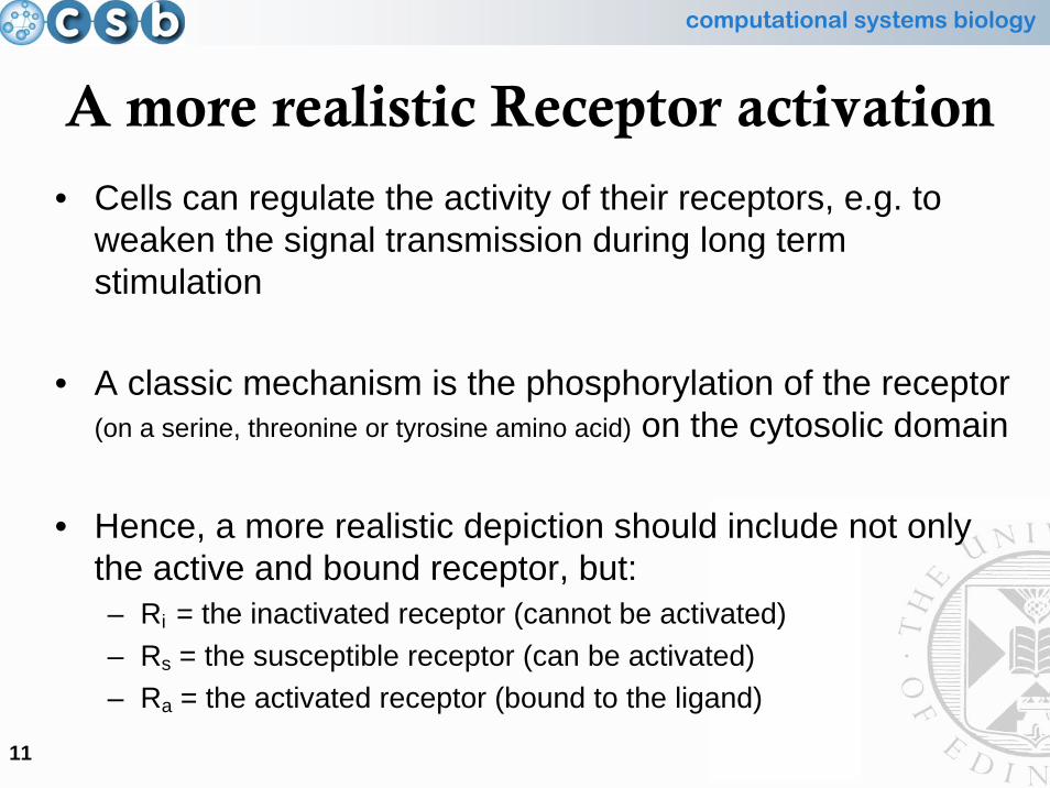
A more realistic Receptor activation
• Cells can regulate the activity of their receptors, e.g. to weaken the signal transmission during long term stimulation
• A classic mechanism is the phosphorylation of the receptor (on a serine, threonine or tyrosine amino acid) on the cytosolic domain
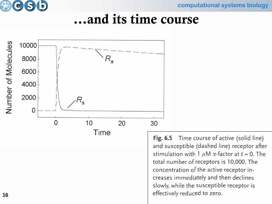
• Hence, a more realistic depiction should include not only the active and bound receptor, but:– Ri = the inactivated receptor (cannot be activated)– Rs = the susceptible receptor (can be activated)– Ra = the activated receptor (bound to the ligand)
computational systems biology
12
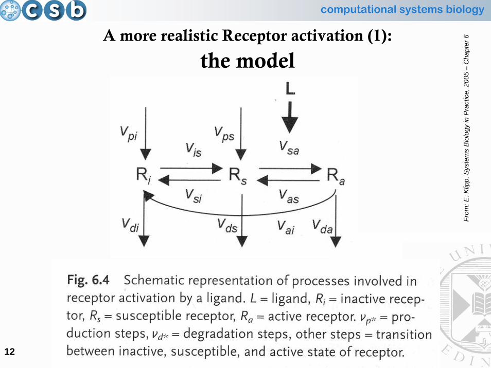
A more realistic Receptor activation (1):
the model
From
: E. K
lipp,
Sys
tem
s B
iolo
gy in
Pra
ctic
e, 2
005
–C
hapt
er 6
computational systems biology
13
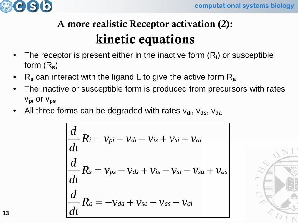
A more realistic Receptor activation (2):
kinetic equations• The receptor is present either in the inactive form (Ri) or susceptible
form (Rs)• Rs can interact with the ligand L to give the active form Ra
• The inactive or susceptible form is produced from precursors with rates vpi or vps
• All three forms can be degraded with rates vdi, vds, vda
aiassadaa
assasiisdspss
aisiisdipii
vvvvRdtd
vvvvvvRdtd
vvvvvRdtd
−−+−=
+−−+−=
++−−=
computational systems biology
14
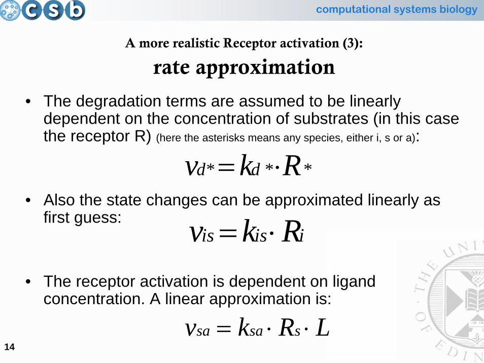
A more realistic Receptor activation (3):
rate approximation
• The degradation terms are assumed to be linearly dependent on the concentration of substrates (in this case the receptor R) (here the asterisks means any species, either i, s or a):
• Also the state changes can be approximated linearly as first guess:
• The receptor activation is dependent on ligand concentration. A linear approximation is:
** Rkv dd* ⋅=
iisis Rkv ⋅=
LRkv ssasa ⋅⋅=

computational systems biology
15
A practical example…
computational systems biology
16
…and its time course
computational systems biology
17
Signalling Paradigm: the structural components
•• G protein cycleG protein cycle
• MAP kinase cascade
computational systems biology
18
G protein
From
: E. K
lipp,
Sys
tem
s B
iolo
gy in
Pra
ctic
e, 2
005
–C
hapt
er 6

computational systems biology
19
Guanosine nucleotide-binding protein(G protein)
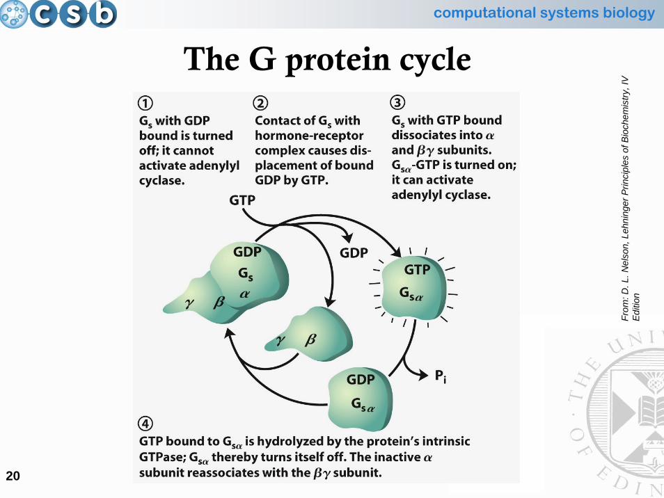
• The G protein is an heterotrimer, consisting of 3 different subunits (alpha, beta and gamma)
• The alpha subunit bound to GDP (guanosine di-[two] phosphate)has high affinity for the beta and gamma subunits
• When it is stimulated by the activated receptor, the alpha subunit exchanges bound GDP for GTP (guanosine tri-[three] phosphate)
• The GTP-bound alpha subunit dissociates from the beta/gamma components, and it binds to a nearby enzyme, altering its activity
• GTP is then hydrolysed to GDP (looses a phosphate group) by the intrinsic GTPase activity of the alpha subunit, that regains itsaffinity for the beta/gamma subunits
computational systems biology
20
The G protein cycle
From
: D. L
. Nel
son,
Leh
ning
er P
rinci
ples
of B
ioch
emis
try, I
V
Editi
on

computational systems biology
21
G protein Coupled Receptors
• The human genome encodes more than 1000 G-protein Coupled Receptors (GPCR), that transduce messages as diverse as light, smells, taste, and hormones
• An example is the beta-adrenergic receptor, that mediates the effects of epinephrine on many tissues:…
computational systems biology
22
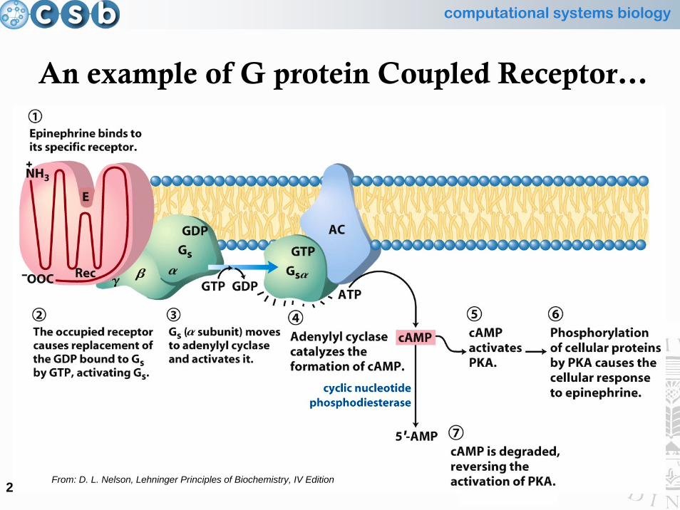
An example of G protein Coupled Receptor…
From: D. L. Nelson, Lehninger Principles of Biochemistry, IV Edition

computational systems biology
23
• An example of signal transduction amplification
… and the following signalling cascade
From: D. L. Nelson, Lehninger Principles of Biochemistry, IV Edition
computational systems biology
24
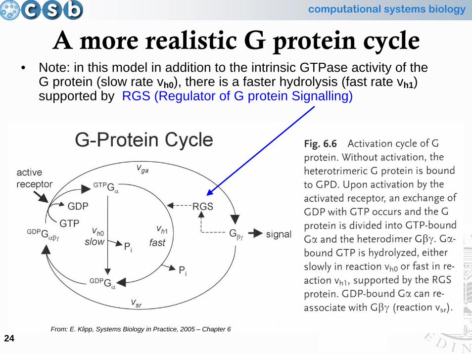
A more realistic G protein cycle• Note: in this model in addition to the intrinsic GTPase activity of the
G protein (slow rate vh0), there is a faster hydrolysis (fast rate vh1) supported by RGS (Regulator of G protein Signalling)
From: E. Klipp, Systems Biology in Practice, 2005 – Chapter 6
computational systems biology
25
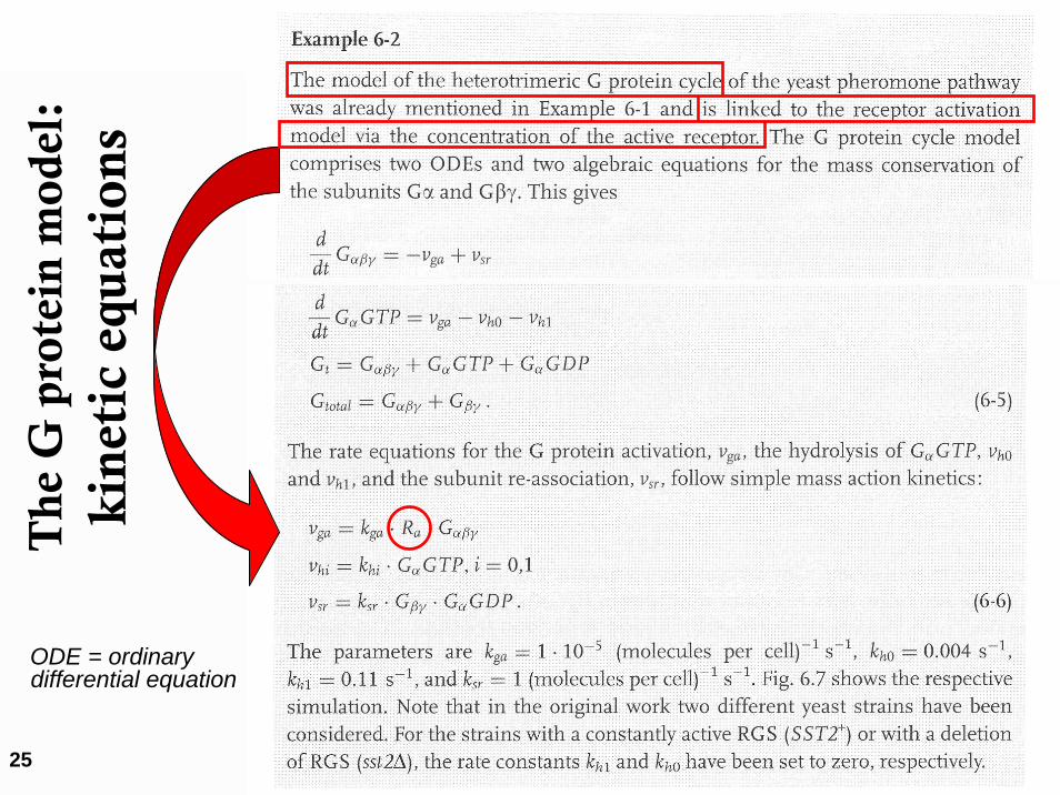
The
G p
rote
in m
odel
:ki
neti
c eq
uati
ons
ODE = ordinary differential equation
computational systems biology
26
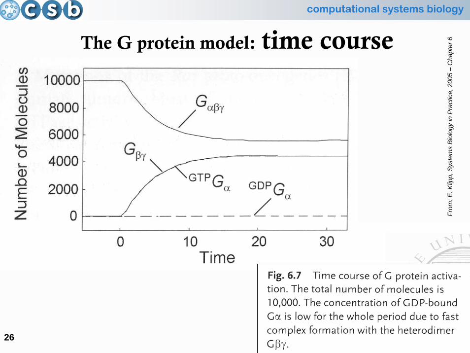
The G protein model: time course
From
: E. K
lipp,
Sys
tem
s B
iolo
gy in
Pra
ctic
e, 2
005
–C
hapt
er 6
computational systems biology
27
Signalling Paradigm: the structural components
• G protein cycle
•• MAP kinase cascadeMAP kinase cascade
computational systems biology
28
MAPK
From
: E. K
lipp,
Sys
tem
s B
iolo
gy in
Pra
ctic
e, 2
005
–C
hapt
er 6
computational systems biology
29
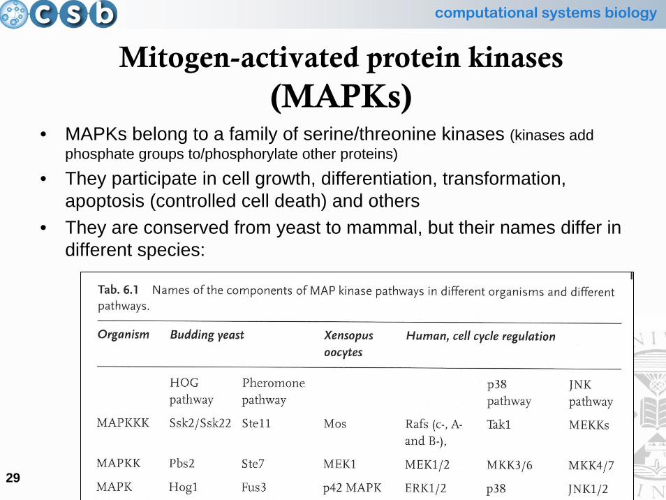
Mitogen-activated protein kinases(MAPKs)
• MAPKs belong to a family of serine/threonine kinases (kinases add phosphate groups to/phosphorylate other proteins)
• They participate in cell growth, differentiation, transformation, apoptosis (controlled cell death) and others
• They are conserved from yeast to mammal, but their names differ in different species:
computational systems biology
30
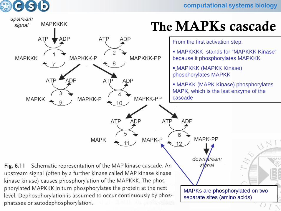
The MAPKs cascadeFrom the first activation step:
MAPKKKK stands for “MAPKKK Kinase”because it phosphorylates MAPKKK
MAPKKK (MAPKK Kinase) phosphorylates MAPKK
MAPKK (MAPK Kinase) phosphorylates MAPK, which is the last enzyme of the cascade
MAPKs are phosphorylated on two separate sites (amino acids)

computational systems biology
31
Reading
• D. L. Nelson, Lehninger Principles of Biochemistry, IV Edition:
– Parts of Chapter 12 on Biosignalling
• E. Klipp, Systems Biology in Practice, Wiley-VCH, 2005:
– Parts of Chapter 6 on Signal Transduction
computational systems biology
32
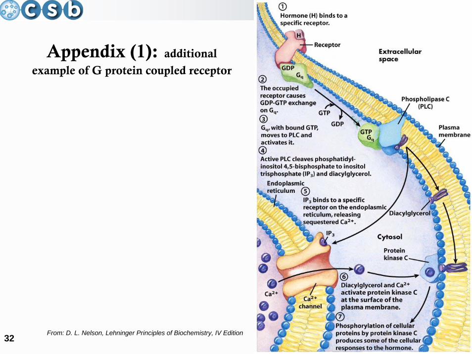
Appendix (1): additional
example of G protein coupled receptor
From: D. L. Nelson, Lehninger Principles of Biochemistry, IV Edition
computational systems biology
33
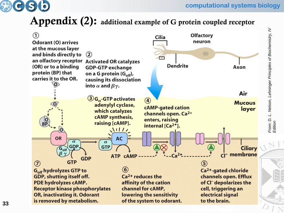
From
: D. L
. Nel
son,
Leh
ning
er P
rinci
ples
of B
ioch
emis
try, I
V
Editi
on
Appendix (2): additional example of G protein coupled receptor


![[VII]. Regulation of Gene Expression Via Signal Transduction Reading List VII: Signal transduction Signal transduction in biological systems.](https://static.fdocuments.net/doc/165x107/56649e385503460f94b28319/vii-regulation-of-gene-expression-via-signal-transduction-reading-list-vii.jpg)