Lecture 7. Multilayer Perceptron. Backpropagation · • Backpropagation ∗Step-by-step derivation...

Semester 2, 2017Lecturer: Andrey Kan

Lecture 7. Multilayer Perceptron. Backpropagation

COMP90051 Statistical Machine Learning

Copyright: University of Melbourne

Statistical Machine Learning (S2 2017) Deck 7

This lecture

• Multilayer perceptron∗ Model structure∗ Universal approximation∗ Training preliminaries

• Backpropagation∗ Step-by-step derivation∗ Notes on regularisation

2


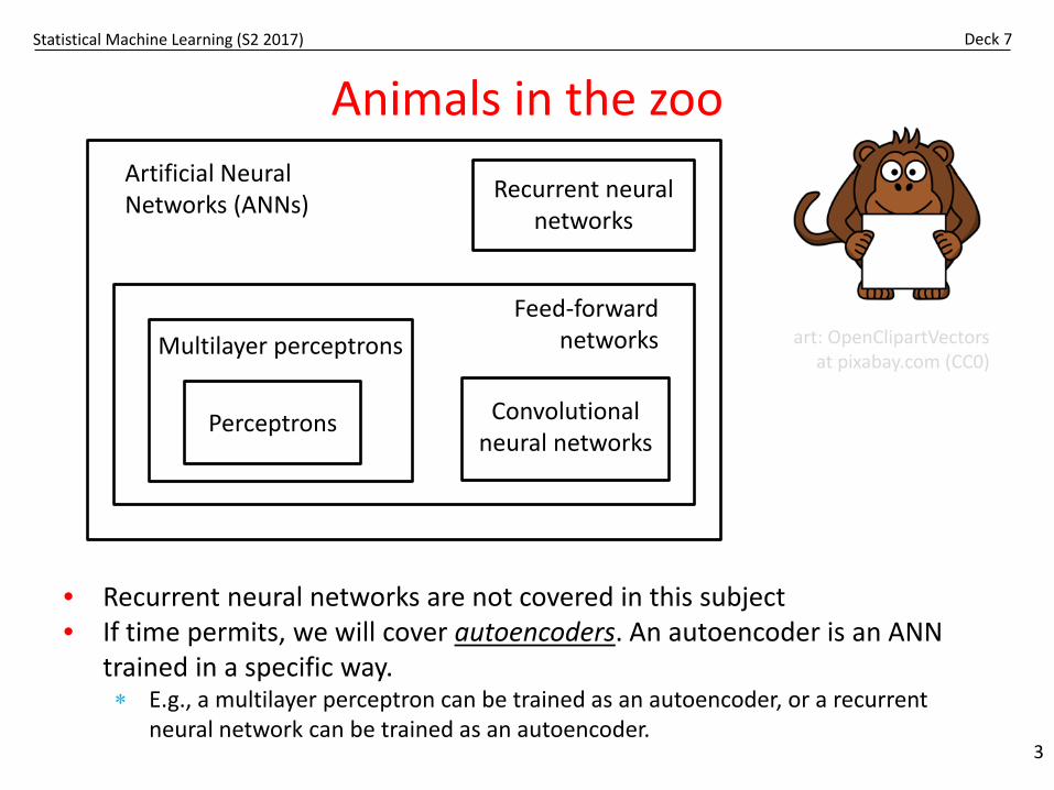
Animals in the zoo

3

Artificial Neural Networks (ANNs)

Feed-forward networksMultilayer perceptrons

Perceptrons Convolutional neural networks

Recurrent neural networks

art: OpenClipartVectorsat pixabay.com (CC0)

• Recurrent neural networks are not covered in this subject• If time permits, we will cover autoencoders. An autoencoder is an ANN

trained in a specific way.∗ E.g., a multilayer perceptron can be trained as an autoencoder, or a recurrent

neural network can be trained as an autoencoder.


Multilayer Perceptron

Modelling non-linearity via function composition

4


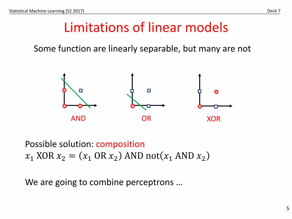
Limitations of linear models

5

AND

Some function are linearly separable, but many are not

OR

Possible solution: composition𝑥𝑥1 XOR 𝑥𝑥2 = 𝑥𝑥1 OR 𝑥𝑥2 AND not 𝑥𝑥1 AND 𝑥𝑥2

XOR

We are going to combine perceptrons …


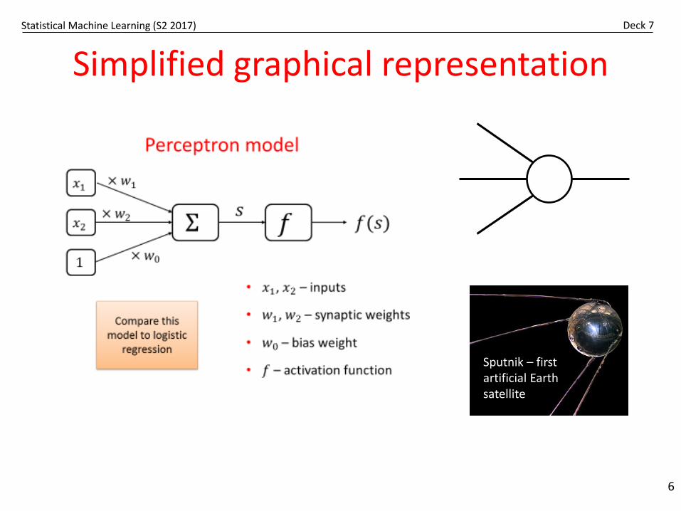
Simplified graphical representation

6

Sputnik – first artificial Earth satellite


Perceptorn is sort of a building block for ANN

7

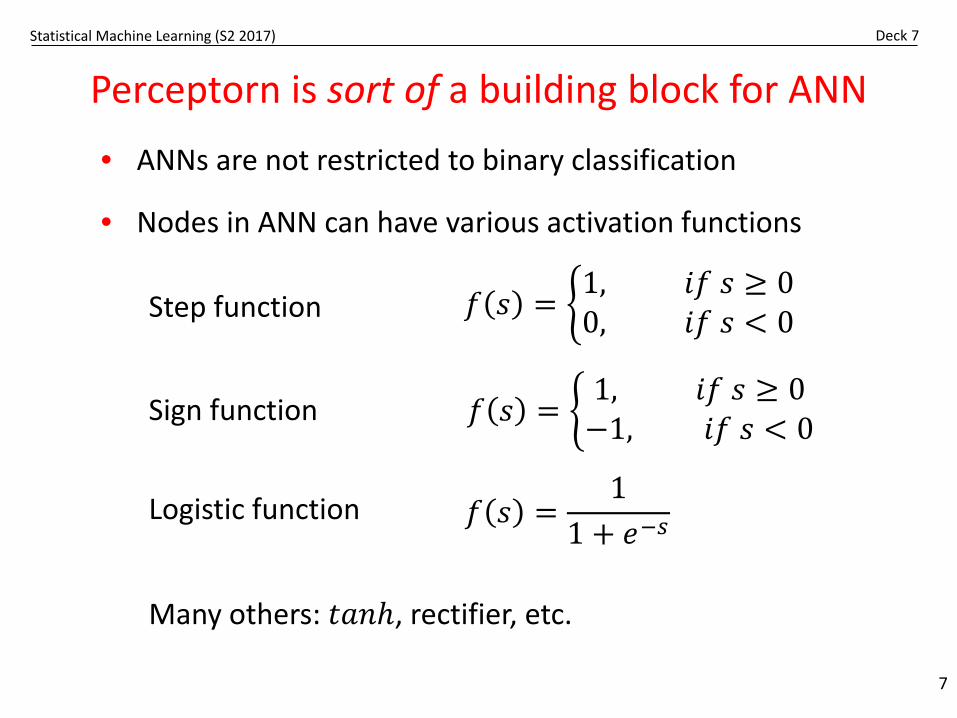
• ANNs are not restricted to binary classification

• Nodes in ANN can have various activation functions

𝑓𝑓 𝑠𝑠 = �1, 𝑖𝑖𝑓𝑓 𝑠𝑠 ≥ 00, 𝑖𝑖𝑓𝑓 𝑠𝑠 < 0

𝑓𝑓 𝑠𝑠 = � 1, 𝑖𝑖𝑓𝑓 𝑠𝑠 ≥ 0−1, 𝑖𝑖𝑓𝑓 𝑠𝑠 < 0

𝑓𝑓 𝑠𝑠 =1

1 + 𝑒𝑒−𝑠𝑠

Step function

Sign function

Logistic function

Many others: 𝑡𝑡𝑡𝑡𝑡𝑡𝑡, rectifier, etc.


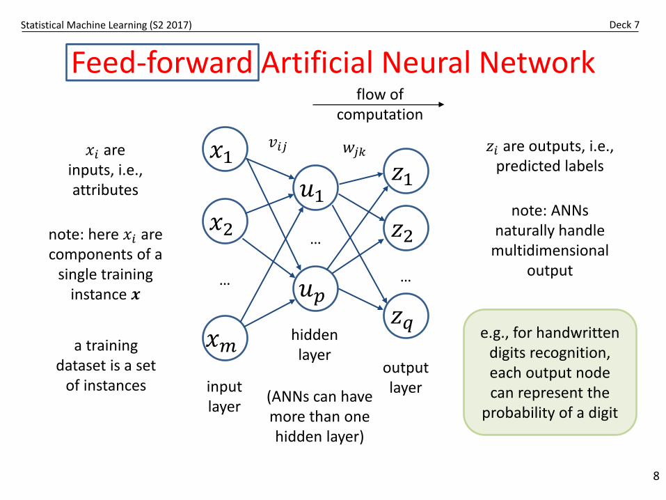
Feed-forward Artificial Neural Network

8

𝑥𝑥1

𝑥𝑥2

𝑥𝑥𝑚𝑚

𝑢𝑢1𝑧𝑧1

𝑧𝑧2

𝑧𝑧𝑞𝑞𝑢𝑢𝑝𝑝…

…

…

input layer

hidden layer

(ANNs can have more than one hidden layer)

output layer

𝑥𝑥𝑖𝑖 are inputs, i.e., attributes

𝑧𝑧𝑖𝑖 are outputs, i.e., predicted labels

note: here 𝑥𝑥𝑖𝑖 are components of a

single training instance 𝒙𝒙

𝑤𝑤𝑗𝑗𝑗𝑗𝑣𝑣𝑖𝑖𝑗𝑗

e.g., for handwritten digits recognition, each output node can represent the

probability of a digit

a training dataset is a set

of instances

note: ANNs naturally handle

multidimensional output

flow of computation


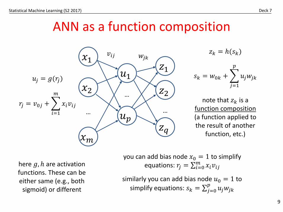
ANN as a function composition

9

𝑥𝑥1

𝑥𝑥2

𝑥𝑥𝑚𝑚

𝑢𝑢1𝑧𝑧1

𝑧𝑧2

𝑧𝑧𝑞𝑞𝑢𝑢𝑝𝑝…

…

…

𝑢𝑢𝑗𝑗 = 𝑔𝑔(𝑟𝑟𝑗𝑗)

𝑟𝑟𝑗𝑗 = 𝑣𝑣0𝑗𝑗 + �𝑖𝑖=1

𝑚𝑚

𝑥𝑥𝑖𝑖𝑣𝑣𝑖𝑖𝑗𝑗

𝑧𝑧𝑗𝑗 = 𝑡(𝑠𝑠𝑗𝑗)

𝑠𝑠𝑗𝑗 = 𝑤𝑤0𝑗𝑗 + �𝑗𝑗=1

𝑝𝑝

𝑢𝑢𝑗𝑗𝑤𝑤𝑗𝑗𝑗𝑗

you can add bias node 𝑥𝑥0 = 1 to simplify equations: 𝑟𝑟𝑗𝑗 = ∑𝑖𝑖=0𝑚𝑚 𝑥𝑥𝑖𝑖𝑣𝑣𝑖𝑖𝑗𝑗here 𝑔𝑔, 𝑡 are activation

functions. These can be either same (e.g., both

sigmoid) or different

note that 𝑧𝑧𝑗𝑗 is a function composition(a function applied to the result of another

function, etc.)

𝑤𝑤𝑗𝑗𝑗𝑗𝑣𝑣𝑖𝑖𝑗𝑗

similarly you can add bias node 𝑢𝑢0 = 1 to simplify equations: 𝑠𝑠𝑗𝑗 = ∑𝑗𝑗=0

𝑝𝑝 𝑢𝑢𝑗𝑗𝑤𝑤𝑗𝑗𝑗𝑗


ANN in supervised learning

10

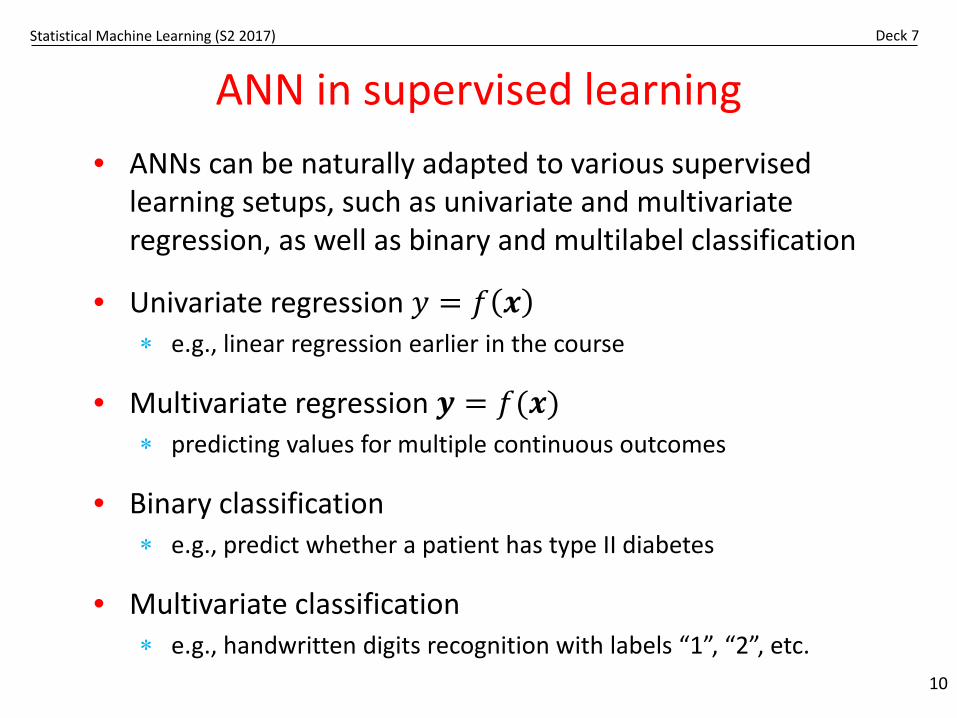
• ANNs can be naturally adapted to various supervised learning setups, such as univariate and multivariate regression, as well as binary and multilabel classification

• Univariate regression 𝑦𝑦 = 𝑓𝑓 𝒙𝒙∗ e.g., linear regression earlier in the course

• Multivariate regression 𝒚𝒚 = 𝑓𝑓(𝒙𝒙)∗ predicting values for multiple continuous outcomes

• Binary classification∗ e.g., predict whether a patient has type II diabetes

• Multivariate classification∗ e.g., handwritten digits recognition with labels “1”, “2”, etc.


The power of ANN as a non-linear model

11

𝑥𝑥

𝑢𝑢1

𝑧𝑧

𝑢𝑢3

𝑢𝑢2

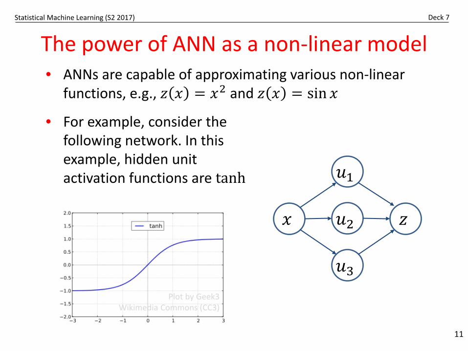
• ANNs are capable of approximating various non-linear functions, e.g., 𝑧𝑧 𝑥𝑥 = 𝑥𝑥2 and 𝑧𝑧 𝑥𝑥 = sin 𝑥𝑥

• For example, consider the following network. In this example, hidden unit activation functions are tanh

Plot by Geek3Wikimedia Commons (CC3)


The power of ANN as a non-linear model

12

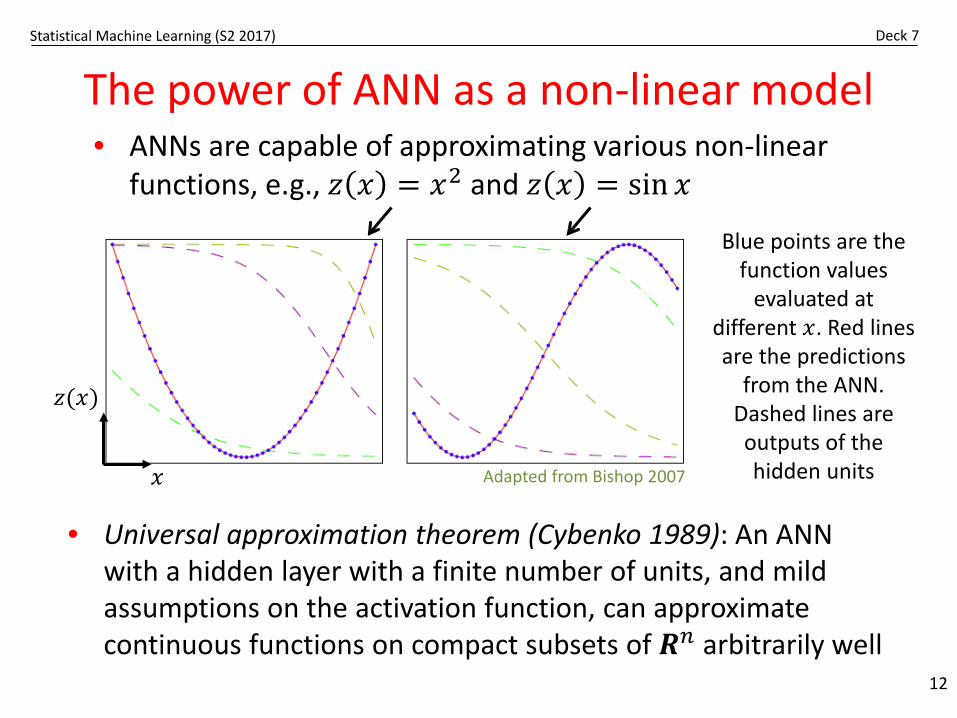
Blue points are the function values

evaluated at different 𝑥𝑥. Red lines are the predictions

from the ANN. Dashed lines are outputs of the hidden units

• Universal approximation theorem (Cybenko 1989): An ANN with a hidden layer with a finite number of units, and mild assumptions on the activation function, can approximate continuous functions on compact subsets of 𝑹𝑹𝑛𝑛 arbitrarily well

Adapted from Bishop 2007𝑥𝑥

𝑧𝑧(𝑥𝑥)

• ANNs are capable of approximating various non-linear functions, e.g., 𝑧𝑧 𝑥𝑥 = 𝑥𝑥2 and 𝑧𝑧 𝑥𝑥 = sin 𝑥𝑥


How to train your dragon network?

13

• You know the drill: Define the loss function and find parameters that minimise the loss on training data

• In the following, we are going to use stochastic gradient descent with a batch size of one. That is, we will process training examples one by one

Adapted from Movie Poster from Flickr user jdxyw (CC BY-SA 2.0)


Training setup: univariate regression

14

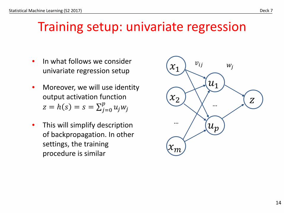
• In what follows we consider univariate regression setup

• Moreover, we will use identity output activation function 𝑧𝑧 = 𝑡 𝑠𝑠 = 𝑠𝑠 = ∑𝑗𝑗=0

𝑝𝑝 𝑢𝑢𝑗𝑗𝑤𝑤𝑗𝑗

• This will simplify description of backpropagation. In other settings, the training procedure is similar

𝑥𝑥1

𝑥𝑥2

𝑥𝑥𝑚𝑚

𝑢𝑢1𝑧𝑧

𝑢𝑢𝑝𝑝…

…

𝑤𝑤𝑗𝑗𝑣𝑣𝑖𝑖𝑗𝑗


Training setup: univariate regression

15

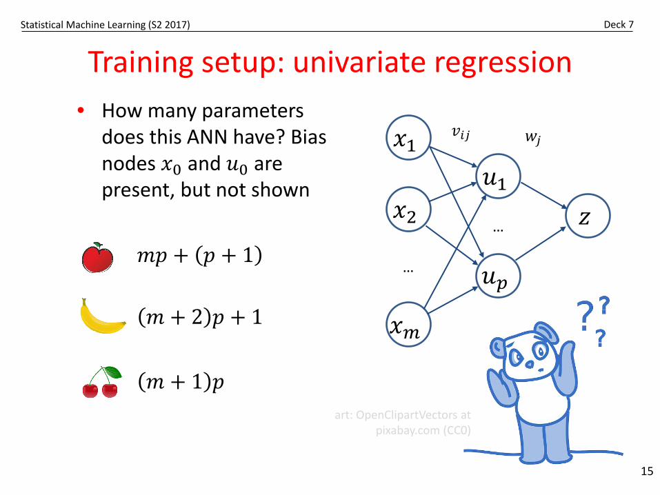
• How many parameters does this ANN have? Bias nodes 𝑥𝑥0 and 𝑢𝑢0 are present, but not shown

𝑥𝑥1

𝑥𝑥2

𝑥𝑥𝑚𝑚

𝑢𝑢1𝑧𝑧

𝑢𝑢𝑝𝑝…

…


art: OpenClipartVectors at pixabay.com (CC0)

𝑚𝑚 + 2 𝑝𝑝 + 1

𝑚𝑚𝑝𝑝 + 𝑝𝑝 + 1

𝑚𝑚 + 1 𝑝𝑝


Loss function for ANN training

16

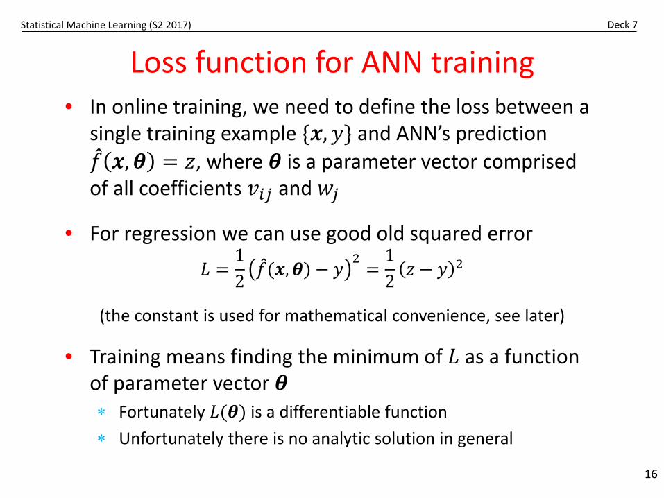
• In online training, we need to define the loss between a single training example {𝒙𝒙,𝑦𝑦} and ANN’s prediction 𝑓𝑓 𝒙𝒙,𝜽𝜽 = 𝑧𝑧, where 𝜽𝜽 is a parameter vector comprised of all coefficients 𝑣𝑣𝑖𝑖𝑗𝑗 and 𝑤𝑤𝑗𝑗

• For regression we can use good old squared error𝐿𝐿 =

12𝑓𝑓(𝒙𝒙,𝜽𝜽) − 𝑦𝑦

2=

12𝑧𝑧 − 𝑦𝑦 2

(the constant is used for mathematical convenience, see later)

• Training means finding the minimum of 𝐿𝐿 as a function of parameter vector 𝜽𝜽∗ Fortunately 𝐿𝐿(𝜽𝜽) is a differentiable function∗ Unfortunately there is no analytic solution in general


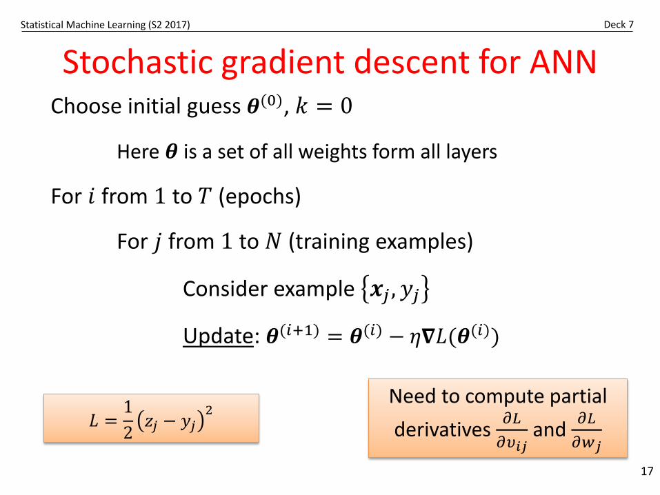
𝐿𝐿 =12𝑧𝑧𝑗𝑗 − 𝑦𝑦𝑗𝑗

2

Stochastic gradient descent for ANNChoose initial guess 𝜽𝜽(0), 𝑘𝑘 = 0

Here 𝜽𝜽 is a set of all weights form all layers

For 𝑖𝑖 from 1 to 𝑇𝑇 (epochs)

For 𝑗𝑗 from 1 to 𝑁𝑁 (training examples)

Consider example 𝒙𝒙𝑗𝑗 , 𝑦𝑦𝑗𝑗

Update: 𝜽𝜽(𝑖𝑖+1) = 𝜽𝜽(𝑖𝑖) − 𝜂𝜂𝛁𝛁𝐿𝐿(𝜽𝜽(𝑖𝑖))

17

Need to compute partial derivatives 𝜕𝜕𝐿𝐿

𝜕𝜕𝜐𝜐𝑖𝑖𝑗𝑗and 𝜕𝜕𝐿𝐿

𝜕𝜕𝑤𝑤𝑗𝑗


Backpropagation

Calculating the gradient of a loss function

18

= “backward propagation of errors”


Backpropagation: start with the chain rule

19

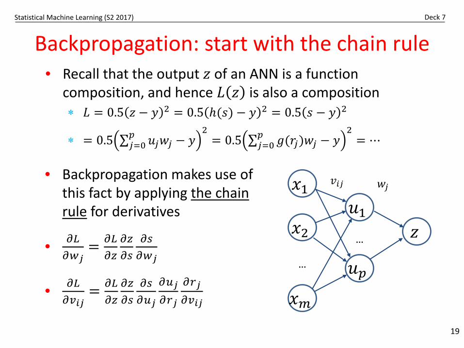
• Recall that the output 𝑧𝑧 of an ANN is a function composition, and hence 𝐿𝐿 𝑧𝑧 is also a composition∗ 𝐿𝐿 = 0.5 𝑧𝑧 − 𝑦𝑦 2 = 0.5 𝑡(𝑠𝑠) − 𝑦𝑦 2 = 0.5 𝑠𝑠 − 𝑦𝑦 2

∗ = 0.5 ∑𝑗𝑗=0𝑝𝑝 𝑢𝑢𝑗𝑗𝑤𝑤𝑗𝑗 − 𝑦𝑦

2= 0.5 ∑𝑗𝑗=0

𝑝𝑝 𝑔𝑔(𝑟𝑟𝑗𝑗)𝑤𝑤𝑗𝑗 − 𝑦𝑦2

= ⋯

• Backpropagation makes use of this fact by applying the chain rule for derivatives

• 𝜕𝜕𝐿𝐿𝜕𝜕𝑤𝑤𝑗𝑗

= 𝜕𝜕𝐿𝐿𝜕𝜕𝑧𝑧

𝜕𝜕𝑧𝑧𝜕𝜕𝑠𝑠

𝜕𝜕𝑠𝑠𝜕𝜕𝑤𝑤𝑗𝑗

• 𝜕𝜕𝐿𝐿𝜕𝜕𝑣𝑣𝑖𝑖𝑗𝑗



𝜕𝜕𝑠𝑠𝜕𝜕𝑢𝑢𝑗𝑗

𝜕𝜕𝑢𝑢𝑗𝑗𝜕𝜕𝑟𝑟𝑗𝑗

𝜕𝜕𝑟𝑟𝑗𝑗𝜕𝜕𝑣𝑣𝑖𝑖𝑗𝑗

𝑥𝑥1

𝑥𝑥2

𝑥𝑥𝑚𝑚

𝑢𝑢1𝑧𝑧

𝑢𝑢𝑝𝑝…

…



Backpropagation: intermediate step

20

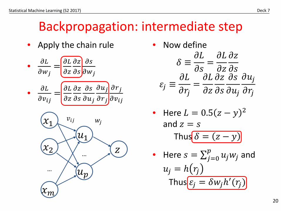
• Apply the chain rule

• 𝜕𝜕𝐿𝐿𝜕𝜕𝑤𝑤𝑗𝑗



𝜕𝜕𝑠𝑠𝜕𝜕𝑤𝑤𝑗𝑗

• 𝜕𝜕𝐿𝐿𝜕𝜕𝑣𝑣𝑖𝑖𝑗𝑗





𝜕𝜕𝑟𝑟𝑗𝑗𝜕𝜕𝑣𝑣𝑖𝑖𝑗𝑗

𝑥𝑥1

𝑥𝑥2

𝑥𝑥𝑚𝑚

𝑢𝑢1𝑧𝑧

𝑢𝑢𝑝𝑝…

…


• Now define

𝛿𝛿 ≡𝜕𝜕𝐿𝐿𝜕𝜕𝑠𝑠

=𝜕𝜕𝐿𝐿𝜕𝜕𝑧𝑧


𝜀𝜀𝑗𝑗 ≡𝜕𝜕𝐿𝐿𝜕𝜕𝑟𝑟𝑗𝑗

=𝜕𝜕𝐿𝐿𝜕𝜕𝑧𝑧




• Here 𝐿𝐿 = 0.5 𝑧𝑧 − 𝑦𝑦 2

and 𝑧𝑧 = 𝑠𝑠Thus 𝛿𝛿 = 𝑧𝑧 − 𝑦𝑦

• Here 𝑠𝑠 = ∑𝑗𝑗=0𝑝𝑝 𝑢𝑢𝑗𝑗𝑤𝑤𝑗𝑗 and

𝑢𝑢𝑗𝑗 = 𝑡 𝑟𝑟𝑗𝑗Thus 𝜀𝜀𝑗𝑗 = 𝛿𝛿𝑤𝑤𝑗𝑗𝑡′(𝑟𝑟𝑗𝑗)


Backpropagation equations

21

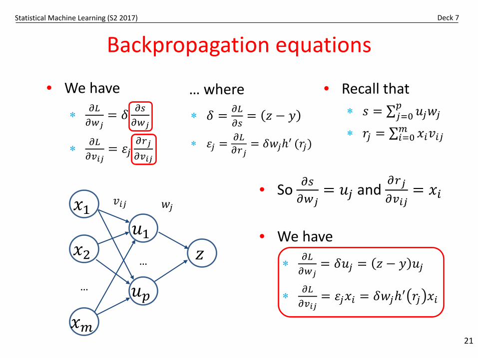
• We have

∗ 𝜕𝜕𝐿𝐿𝜕𝜕𝑤𝑤𝑗𝑗

= 𝛿𝛿 𝜕𝜕𝑠𝑠𝜕𝜕𝑤𝑤𝑗𝑗

∗ 𝜕𝜕𝐿𝐿𝜕𝜕𝑣𝑣𝑖𝑖𝑗𝑗

= 𝜀𝜀𝑗𝑗𝜕𝜕𝑟𝑟𝑗𝑗𝜕𝜕𝑣𝑣𝑖𝑖𝑗𝑗

𝑥𝑥1

𝑥𝑥2

𝑥𝑥𝑚𝑚

𝑢𝑢1𝑧𝑧

𝑢𝑢𝑝𝑝…

…


… where

∗ 𝛿𝛿 = 𝜕𝜕𝐿𝐿𝜕𝜕𝑠𝑠

= 𝑧𝑧 − 𝑦𝑦

∗ 𝜀𝜀𝑗𝑗 = 𝜕𝜕𝐿𝐿𝜕𝜕𝑟𝑟𝑗𝑗

= 𝛿𝛿𝑤𝑤𝑗𝑗𝑡′ (𝑟𝑟𝑗𝑗)

• So 𝜕𝜕𝑠𝑠𝜕𝜕𝑤𝑤𝑗𝑗

= 𝑢𝑢𝑗𝑗 and 𝜕𝜕𝑟𝑟𝑗𝑗𝜕𝜕𝑣𝑣𝑖𝑖𝑗𝑗

= 𝑥𝑥𝑖𝑖

• We have


= 𝛿𝛿𝑢𝑢𝑗𝑗 = 𝑧𝑧 − 𝑦𝑦 𝑢𝑢𝑗𝑗


= 𝜀𝜀𝑗𝑗𝑥𝑥𝑖𝑖 = 𝛿𝛿𝑤𝑤𝑗𝑗𝑡′ 𝑟𝑟𝑗𝑗 𝑥𝑥𝑖𝑖

• Recall that∗ 𝑠𝑠 = ∑𝑗𝑗=0

𝑝𝑝 𝑢𝑢𝑗𝑗𝑤𝑤𝑗𝑗∗ 𝑟𝑟𝑗𝑗 = ∑𝑖𝑖=0𝑚𝑚 𝑥𝑥𝑖𝑖𝑣𝑣𝑖𝑖𝑗𝑗


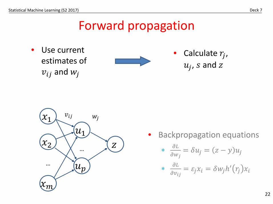
Forward propagation

22

• Use current estimates of 𝑣𝑣𝑖𝑖𝑗𝑗 and 𝑤𝑤𝑗𝑗

𝑥𝑥1

𝑥𝑥2

𝑥𝑥𝑚𝑚

𝑢𝑢1𝑧𝑧

𝑢𝑢𝑝𝑝…

…


• Calculate 𝑟𝑟𝑗𝑗, 𝑢𝑢𝑗𝑗, 𝑠𝑠 and 𝑧𝑧

• Backpropagation equations






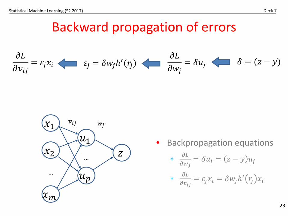
Backward propagation of errors

23

𝑥𝑥1

𝑥𝑥2

𝑥𝑥𝑚𝑚

𝑢𝑢1𝑧𝑧

𝑢𝑢𝑝𝑝…

…


𝛿𝛿 = (𝑧𝑧 − 𝑦𝑦)

• Backpropagation equations





𝜕𝜕𝐿𝐿𝜕𝜕𝑤𝑤𝑗𝑗

= 𝛿𝛿𝑢𝑢𝑗𝑗𝜕𝜕𝐿𝐿𝜕𝜕𝑣𝑣𝑖𝑖𝑗𝑗

= 𝜀𝜀𝑗𝑗𝑥𝑥𝑖𝑖 𝜀𝜀𝑗𝑗 = 𝛿𝛿𝑤𝑤𝑗𝑗𝑡′(𝑟𝑟𝑗𝑗)


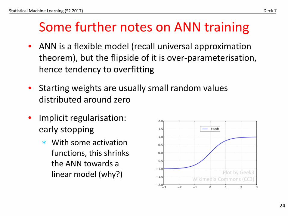
Some further notes on ANN training

24

• ANN is a flexible model (recall universal approximation theorem), but the flipside of it is over-parameterisation, hence tendency to overfitting

• Starting weights are usually small random values distributed around zero

Plot by Geek3Wikimedia Commons (CC3)

• Implicit regularisation: early stopping∗ With some activation

functions, this shrinks the ANN towards a linear model (why?)


Explicit regularisation

25

• Alternatively, an explicit regularisation can be used, much like in ridge regression

• Instead of minimising the loss 𝐿𝐿, minimise regularised function 𝐿𝐿 + 𝜆𝜆 ∑𝑖𝑖=0𝑚𝑚 ∑𝑗𝑗=1

𝑝𝑝 𝑣𝑣𝑖𝑖𝑗𝑗2 + ∑𝑗𝑗=0𝑝𝑝 𝑤𝑤𝑗𝑗2

• This will simply add 2𝜆𝜆𝑣𝑣𝑖𝑖𝑗𝑗 and 2𝜆𝜆𝑤𝑤𝑗𝑗 terms to the partial derivatives

• With some activation functions this also shrinks the ANN towards a linear model


This lecture

• Multilayer perceptron∗ Model structure∗ Universal approximation∗ Training preliminaries

• Backpropagation∗ Step-by-step derivation∗ Notes on regularisation

26

Lecture 7. Multilayer Perceptron. Backpropagation · • Backpropagation ∗Step-by-step derivation...

Documents

Transcript of Lecture 7. Multilayer Perceptron. Backpropagation · • Backpropagation ∗Step-by-step derivation...