Lecture 6: Technology, Geography and Tradegregory.corcos.free.fr/M2/lecture 6.pdf ·...

Introduction The EK model Empirical Applications Conclusion Appendix

Lecture 6: Technology, Geography and Trade

Gregory [email protected]

Isabelle Mé[email protected]

International TradeUniversité Paris-Saclay Master in Economics, 2nd year.

16 November 2016

G. Corcos & I. Méjean (Ecole polytechnique) International Trade: Lecture 6 1 / 52

mailto:[email protected]

mailto:[email protected]


Introduction

Ricardo and HO theories (Lectures 2-4) :I Specialization according to comparative advantageI Inter-industry trade between countries that differ in terms of

technologies (Ricardo) or endowments (HO)I Gains from trade due to a better allocation of resources

Limited empirical support (Lecture 5)I Missing features in HOV can partially explain poor empirical

performancesI In any case, the R2 of such regressions is small

No (explicit) role for geographyI Hardly reconcilable with the gravity equation.



The gravity equation

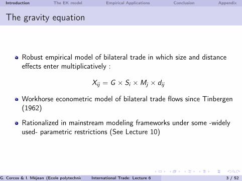
Robust empirical model of bilateral trade in which size and distanceeffects enter multiplicatively :

Xij = G × Si ×Mj × dij

Workhorse econometric model of bilateral trade flows since Tinbergen(1962)

Rationalized in mainstream modeling frameworks under some -widelyused- parametric restrictions (See Lecture 10)



Trade and the size of countries

Japanese exports in the EU Japan imports from the EUFigure 1: Trade is proportional to size

(a) Japan’s exports to EU, 2006 (b) Japan’s imports from EU, 2006

MLT

ESTCYP

LVA

LTUSVN

SVK

HUNCZE

PRT

FINIRLGRC

DNK

AUTPOL

SWE

BELNLD

ESP ITAFRA

GBRDEU

slope = 1.001fit = .85

.05

.1.5

15

10Ja

pan'

s 20

06 e

xpor

ts (G

RC =

1)

.05 .1 .5 1 5 10GDP (GRC = 1)

MLT

EST

CYP

LVA

LTU

SVN

SVK

HUNCZE

PRT

FIN

IRL

GRC

DNKAUT

POL

SWEBELNLD ESP

ITAFRAGBR

DEU

slope = 1.03fit = .75

.51

510

5010

0Ja

pan'

s 20

06 im

ports

(GRC

= 1

)

.05 .1 .5 1 5 10GDP (GRC = 1)

in concert to establish robustness. In recent years, estimation has become just a first step before a

deeper analysis of the implications of the results, notably in terms of welfare. We try to facilitate

diffusion of best-practice methods by illustrating their application in a step-by-step cookbook mode

of exposition.

1.1 Gravity features of trade data

Before considering theory, we use graphical displays to lay out the factual basis for taking gravity

equations seriously. The first key feature of trade data that mirrors the physical gravity equation

is that exports rise proportionately with the economic size of the destination and imports rise in

proportion to the size of the origin economy. Using GDP as the economy size measure, we illustrate

this proportionality using trade flows between Japan and the European Union. The idea is that the

European Union’s area is small enough and sufficiently far from Japan that differences in distance

to Japan can be ignored. Similarly because the EU is a customs union, each member applies the

same trade policies on Japanese imports. Japan does not share a language, religion, currency or

colonial history with any EU members either.

Figure 1 (a) shows Japan’s bilateral exports on the vertical axis and (b) shows its imports.

The horizontal axes of both figures show the GDP (using market exchange rates) of the EU trade

partner. The trade flows and GDPs are normalized by dividing by the corresponding value for

Greece (a mid-size economy).2 The lines show the predicted values from a simple regression of log

2The trade data come from DoTS and the GDPs come from WDI. The web appendix provides more informationon sources of gravity data.

3

Correlation between the Japan-EU trade and the size of partners. The x-axismeasure the GDP of each EU members, in relative terms with respect to theGreek one. The y-axis measure the size of Japanese exports in each country(left-hand side) a,d the volume of Japanese imports from each country (right-hand side), again expressed in relative terms with respect to Greece. Data arefor 2006. Source : Head & Mayer (2014).



Trade and distance

French exports French importsFigure 2: Trade is inversely proportional to distance

(a) France’s exports (2006) (b) France’s imports (2006)

slope = -.683fit = .22

.005

.05

.1.5

15

10E

xpor

ts/P

artn

er's

GD

P (

%, l

og s

cale

)

500 1000 2000 5000 10000 20000Distance in kms

EU25

Euro

Colony

Francophone

other

slope = -.894fit = .2

.005

.05

.1.5

15

1025

Impo

rts/

Par

tner

's G

DP

(%

, log

sca

le)

500 1000 2000 5000 10000 20000Distance in kms

EU25

Euro

Colony

Francophone

other

trade flow on log GDP. For Japan’s exports, the GDP elasticity is 1.00 and it is 1.03 for Japan’s

imports. The near unit elasticity is not unique to the 2006 data. Over the decade 2000–2009, the

export elasticity averaged 0.98 and its confidence intervals always included 1.0. Import elasticities

averaged a somewhat higher 1.11 but the confidence intervals included 1.0 in every year except

2000 (when 10 of the EU25 had yet to join). The gravity equation is sometimes disparaged on

the grounds that any model of trade should exhibit size effects for the exporter and importer.

What these figures and regression results show is that the size relationship takes a relatively precise

form—one that is predicted by most, but not all, models.

Figure 2 illustrates the second key empirical relationship embodied in gravity equations—the

strong negative relationship between physical distance and trade. Since we have just seen that GDPs

enter gravity with a coefficient very close to one, one can pass GDP to the left-hand-side, and show

how bilateral imports or exports as a fraction of GDP varies with distance. Panels (a) and (b) of

Figure 2 graph recent export and import data from France. These panels show deviations from the

distance effect associated with Francophone countries, former colonies, and other members of the

EU or of the Eurozone. The graph expresses the “spirit” of gravity: it identifies deviations from

a benchmark taking into account GDP proportionality and systematic negative distance effects.

Those deviations have become the subject of many separate investigations.

This paper is mainly organized around topics with little attention paid to the chronology of

when ideas appeared in the literature. But we do not think the history of idea development should

be overlooked entirely. Therefore in the next section we give our account of how gravity equations

went from being nearly ignored by trade economists to becoming a focus of research published in

4

Correlation between the volume of trade and the distance between partners.The x-axis is the distance from France, expressed in kilometers. The x-axismeasures the size of French exports (left-hand side) and the size of Frenchimports (right-hand side), both expressed in relative terms with respect ot thedestination country’s GDP. Data are for 2006. Source : Head & Mayer (2014).



The Eaton and Kortum (2002) Model

Eaton & Kortum (2002) : neoclassical trade model in whichI Comparative advantage arises randomlyI Technological advantage interacts with geography to shape

comparative advantageI Gravity equation arises structurally

The EK model has been used in quantitative exercises on :I gains from trade liberalization (e.g. zero MFN tariffs, NAFTA)I the importance/evolution of Ricardian comparative advantageI the fall in trade during the 2008-2009 recessionI the US trade deficit and exchange rate adjustmentI the volatility of trade and GDP...



Outline of this Lecture

Detailed presentation of the Eaton-Kortum model

Some extensions

Estimation of Eaton-Kortum

Numerical applications



The Eaton-Kortum model

See analytical details in EatonKortumAnalytics.pdf



Main features

Ricardian model (differences in technology) with geography (barriersto trade).The model yields a gravity equation which relates bilateral tradevolumes to deviations from purchasing power parity, technology andgeographic barriers.The model can be estimated structurally.



Assumptions

I countries (i = 1...I )Continuum of goods j ∈ [0, 1]

CES preferences in each country i :

Ui =

[∫ 1

0Qi (j)

σ−1σ dj

] σσ−1

demand

Goods produced with a bundle of inputs whose price is homogenouswithin countries ci (first taken as exogenous)Iceberg trade costs dni > 1. Without loss of generality dii = 1.Cross-border arbitrage implies : dni ≤ dnkdki



Assumptions (ii)

Country i ’s efficiency in producing good j : zi (j)⇒ CIF price of good j produced in country i and sold in country n :

pni (j) =ci

zi (j)︸︷︷︸Unit cost

dni︸︷︷︸Trade barrier

optimal price

Perfect competition across suppliers⇒ Price actually paid in country n for good j :

pn(j) = min{pni (j); i = 1...I}

Note : most results continue to hold with Bertrand competition.



Assumptions (iii)

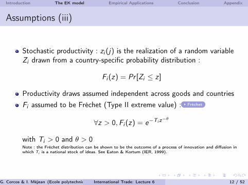
Stochastic productivity : zi (j) is the realization of a random variableZi drawn from a country-specific probability distribution :

Fi (z) = Pr [Zi ≤ z ]

Productivity draws assumed independent across goods and countriesFi assumed to be Fréchet (Type II extreme value) : Fréchet

∀z > 0,Fi (z) = e−Tiz−θ

with Ti > 0 and θ > 0Note : the Fréchet distribution can be shown to be the outcome of a process of innovation and diffusion inwhich Ti is a national stock of ideas. See Eaton & Kortum (IER, 1999).



Interpretation

Fi (z) = e−Tiz−θ

0

0.1

0.2

0.3

0.4

0.5

0.6

0.7

0.8

0.9

1

Benchmark in red. Doubling of Ti inblue / of θ in green

Ti captures absoluteadvantage. The higher Ti , thehigher that country’s mean z : iis more likely to draw a high zfor each product j .θ captures the extent ofcomparative advantage. Thehigher θ, the lower Var(z) :trade will be less driven bycomparative advantage.



Price distribution

Distribution of prices offered by country i in country n :

Gni (p) ≡ Pr [Pni ≤ p] = 1− e−Ti (cidni )−θpθ

Country n’s actual distribution of prices :

Gn(p) ≡ Pr [Pn ≤ p]

= 1−∏i

[1− Gni (p)]

= 1− e−Φnpθ

where Φn ≡∑

i Ti (cidni )−θ

details



Price distribution

Gn(p) = 1− e−Φnpθ , Φn ≡∑i

Ti (cidni )−θ

Distribution of prices governed byStates of technology around the world {Ti},

Input costs around the world {ci},Geographic barriers {dni}

- If dni = 1,∀n, i then Φn = Φ,∀n (Law of One Price)- If dni →∞,∀i then Φn = Tnc

−θn (Autarky)

⇒ Φn represents the strength of competition that any firm will encounterin country n



Bilateral trade

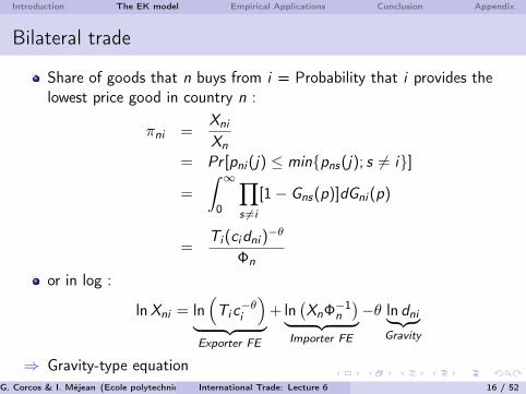
Share of goods that n buys from i = Probability that i provides thelowest price good in country n :

πni =Xni

Xn

= Pr [pni (j) ≤ min{pns(j); s 6= i}]

=

∫ ∞0

∏s 6=i

[1− Gns(p)]dGni (p)

=Ti (cidni )

−θ

Φn

or in log :

lnXni = ln(Tic−θi

)︸︷︷︸Exporter FE

+ ln(XnΦ−1n

)︸︷︷︸Importer FE

−θ ln dni︸︷︷︸Gravity

⇒ Gravity-type equationG. Corcos & I. Méjean (Ecole polytechnique) International Trade: Lecture 6 16 / 52


Bilateral trade (ii)

EK structural interpretation of the gravity equation :The trade barriers coefficient relates to heterogeneity in productivity :

⇒ The greater heterogeneity among producers of a commodity (lower θ),the stronger the cost advantage of the lowest cost supplier, the morelikely he remains the lowest cost supplier when trade costs increase.

⇒ Trade flows respond to geographic barriers at the extensive margin :As a source becomes more expensive or remote, it exports a narrowerrange of goods [as in Dornbusch et al. (1977)].



Bilateral trade (iii)

Country i ’s normalized import share in country n :

Sni ≡Xni/Xn

Xii/Xi=

Φi

Φnd−θni =

(pidnipn

)−θAlways lower than one due to the triangle inequality (the maximumvalue for pn is pidni )As overall prices in market n fall relative to prices in market i(↑ pi/pn) or as n becomes more isolated from i (↑ dni ), i ’s normalizedshare in n declinesA higher θ means comparative advantage forces weaken relative totrade costs : normalized import shares become more elastic.



General equilibrium solution

Suppose production is linear in labor (EK has intermediate inputs) :

ci = wi

⇒ Price levels as a function of wages :

pn = γ

[∑i

Ti (dniwi )−θ

]−1/θ

where γ ≡[Γ(θ+1−σ

θ

)]1/(1−σ)price index

⇒ Trade shares as a function of wages and prices :

Xni

Xn= Ti

(γdniwi

pn

)−θG. Corcos & I. Méjean (Ecole polytechnique) International Trade: Lecture 6 19 / 52


General equilibrium solution

To close the model, one needs to solve for equilibrium wages acrosscountriesThis is the trickier part of the exercise ⇒ Numerical solutionsAdditional simplifying assumptions can help solve the model :Exogenous labor supply, Wages determined in the nonmanufacturingsector, Trade balance.



Extensions : Multiple sectors

Costinot, Donaldson & Komunjer (2012) reinterpret EK’s model in thecontext of a multi-country, multi-sector worldK industries/goods in each country (k = 1, ...,K ). Within eachindustry, a continuum of varieties is produced according to thetechnology described above.With multiple sectors, Ti now has a sector dimension (but, crucially, θremains common to all countries and industries...) :

F ki (z) = e−T

ki z−θ



Extensions : Multiple sectors (ii)

The model predicts trade patterns at the industry-country pair level.For any importer j and any pair of exporters i , i ′ 6= j , the ranking ofrelative fundamental productivities determines the ranking of exports :

T 1i

T 1i ′≤ ... ≤

TKi

TKi ′⇒

X 1ji

X 1ji ′≤ ... ≤

XKji

XKji ′

In a 2-country world without heterogeneity, that ranking would imply

z1i (j)

z1i ′(j)< ... <

zKi (j)

zKi ′ (j)

i would specialize in high-k goods and i ′ in low-k goods, just as inDornbusch et al. (1977).



Extensions : Multiple sectors (iii)

In this model with stochastic (Fréchet) productivity differences, wehave :

T 1i

T 1i ′≤ ... ≤

TKi

TKi ′⇒

z1i (j)

z1i ′(j)� ... �

zKi (j)

zKi ′ (j)

where � denotes first-order stochastic dominance.Country i ′ is not expected to specialize in high k goods, but toproduce and export relatively more of these goods.Unlike Dornbusch et al. (1977) here we can predict trade patterns formore than 2 countries.



Extensions : Imperfect Competition

Bernard, Eaton, Jensen & Kortum (2003) extend EK to allow forimperfect competition between varietiesWith imperfect competition, consumer prices are above marginal costsModel predicts a distribution of mark-ups in each market, that isbounded above by the Dixit-Stiglitz constant mark-upAdditional predictions on within-country heterogeneity in prices,productivities, etc



Bringing the Model to the Data

The model can be estimated to quantitatively assess the role ofRicardian advantages in driving international trade.Structural parameters θ and {Ti} must be estimated.Once those parameters are estimated, it is possible to run variouscounterfactuals.



Example : EK Estimation of θ

Bilateral trade in manufactures among 19 OECD countries in 1990(342 bilateral relationships Xni )Absorption of manufactures as a measure of Xn (STAN, OECD)Proxy for trade barriers :

- Distance and other geographic barriers- Retail price differentials measured at the product level (WB) :Interpreted as a sample of pi (j), used to calculate relative prices, whichare theoretically bounded above by bilateral trade costs :

lnpidnipn'=

max2j{rni (j)}mean{rni (j)}

= Dni

rni (j) = ln pn(j)− ln pi (j) relative price of commodity j⇒ exp(Dni ) price index in destination n that would prevail if everythingwas purchased from i , relative to the actual price index in n



Estimating θ, EK Method 1

Normalized import shares and relative pricestechnology, geography, and trade 1755

Figure 2.—Trade and prices.

we use this value for ! in exploring counterfactuals. This value of ! implies astandard deviation in efficiency (for a given state of technology T ) of 15 percent.In Section 5 we pursue two alternative strategies for estimating !, but we firstcomplete the full description of the model.

4� equilibrium input costs

Our exposition so far has highlighted how trade flows relate to geographyand to prices, taking input costs ci as given. In any counterfactual experiment,however, adjustment of input costs to a new equilibrium is crucial.To close the model we decompose the input bundle into labor and intermedi-

ates. We then turn to the determination of prices of intermediates, given wages.Finally we model how wages are determined. Having completed the full model,we illustrate it with two special cases that yield simple closed-form solutions.

4�1� Production

We assume that production combines labor and intermediate inputs, withlabor having a constant share 2.28 Intermediates comprise the full set of goods

28 We ignore capital as an input to production and as a source of income, although our intermediateinputs play a similar role in the production function. Baxter (1992) shows how a model in whichcapital and labor serve as factors of production delivers Ricardian implications if the interest rate iscommon across countries.

Source : Eaton & Kortum, 2002. Unconditional correlation -0.4

Model : Xni/Xn

Xii/Xi=(

pi dnipn

)−θEstimated θ (method-of-moments) : θ =

∑n

∑i ln

Xni/XnXii/Xi∑

n

∑i [ln dni−ln Pi+ln Pn ]

⇒ θ = 8.28

→ Standard deviation in efficiency at given T= 15%



Counterfactuals

Once estimated, the model can be used to run counterfactuals :What are the welfare gains from trade ? (Arkolakis et al, 2012)What is the impact of multilateral/unilateral tariff eliminations ?(Caliendo & Parro, 2015, Alvarez &Lucas 2007)How much does trade spread the benefit of local improvements intechnology ?By how much should US real wages fall to restore current accountbalance ? (Dekle et al. 2007)



Application : Evaluating the gains from NAFTA

Caliendo & Parro (2015) use a variant of the Eaton-Kortum model toevaluate the trade and welfare impact of NAFTA.

NAFTA : A free trade area between the US, Mexico and Canada- Enhance trade within the area / Divert existing trade between the areaand the RoW

- Increase welfare : Access to cheaper consumption goods plus increasedcompetitiveness through a drop in input prices

→ Potentially important Ricardian gains since the 3 countries have verydifferent production structures

Main insights :I Important role of sectoral IO linkages to amplify the trade and welfare

effect of the partnership



Theoretical framework

i. Multiple sectors :

Ui =K∏

k=1

Qkiαki ,

K∑k=1

αki = 1, Qk

i =

[∫ 1

0Qk

i (j)σk−1σk dj

] σk

σk−1

ii. Input-Output linkages :

cki = wγkii

K∏k ′=1

Pk ′i

γk,k′

i ,K∑

k=1

γk,k′

i = 1− γki

iii. Non tradable sectors :

dkni = +∞ for some k

iv. Sector-specific productivity distributions (Fréchet) :

F ki (z) = e−T

ki z−θk



Analytical predictions

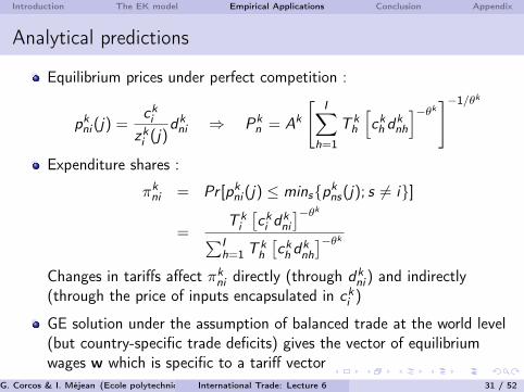
Equilibrium prices under perfect competition :

pkni (j) =cki

zki (j)dkni ⇒ Pk

n = Ak

[I∑

h=1

T kh

[ckh d

knh

]−θk]−1/θkExpenditure shares :

πkni = Pr [pkni (j) ≤ mins{pkns(j); s 6= i}]

=T ki

[cki d

kni

]−θk∑Ih=1 T

kh

[ckh d

knh

]−θkChanges in tariffs affect πkni directly (through dk

ni ) and indirectly(through the price of inputs encapsulated in cki )

GE solution under the assumption of balanced trade at the world level(but country-specific trade deficits) gives the vector of equilibriumwages w which is specific to a tariff vector



Impact of trade liberalization

Equilibrium in relative changes implies :

lnwn

Pn

= −K∑

k=1

αkn

θkln πk

nn︸︷︷︸Final goods

−K∑

k=1

αkn

θk1− γk

n

γkn

ln πknn︸︷︷︸

Intermediate goods

−K∑

k=1

αkn

γknln

J∏l=1

(P ln/P

kn

)γ l,kn

︸︷︷︸Sectoral Linkages

ln πkni = −θk

[ln cki + ln dk

ni − ln Pkn

]where x = dx/x , {cki } and {Pk

n } are non-linear functions of {wn}and {dk

ni}Impact of trade liberalization on real wages can be summarized by theimpact it has on domestic shares ({πknn}) and sectoral price indices({Pk

n })



Impact of trade liberalization (ii)

Trade liberalization increases real wages by reducing the sectoralshares of domestic consumption (ln πknn), i.e.

i. Giving consumers access to cheaper imported goodsii. Reducing the cost of same sector imported inputs (Only role of

intermediates if γkn 6= 1 and γk,kn = 1− γkniii. Reducing the cost of imported inputs for other sectors (when

γk,kn 6= 1− γkn )

Changes in real wages do not directly map into changes in welfare inthis model because of trade deficits (Dn) and tariff revenues (Rn) :

ln Wn = lnIn

Pn

=wnLnIn

lnwn

Pn

+Rn

Inln

Rn

Pn

+Dn

Inln

Dn

Pn



Welfare Impact

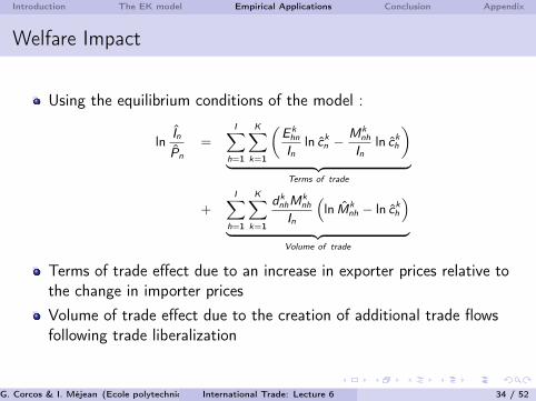
Using the equilibrium conditions of the model :

lnIn

Pn

=I∑

h=1

K∑k=1

(E khn

Inln ckn −

Mknh

Inln ckh

)︸︷︷︸

Terms of trade

+I∑

h=1

K∑k=1

dknhM

knh

In

(ln Mk

nh − ln ckh)

︸︷︷︸Volume of trade

Terms of trade effect due to an increase in exporter prices relative tothe change in importer pricesVolume of trade effect due to the creation of additional trade flowsfollowing trade liberalization



Empirical strategy

Calibration of the observed parameters :I {πk

ni} calibrated using trade and production dataI {αk

i } fitted to data on sectoral absorptionI {γki } and {γ

k,k′

i } fitted to IO tables

Estimation of the unobserved parameters {θk} :

lnX kniX

kimX

kmn

X kinX

kmiX

knm

= −θk lndknid

kimd

kmn

dkind

kmid

knm

ln dkni = ln(1 + τkni ) + νkni + µkn + δki + εkni , νkni = νkin

⇒ lnX kniX

kimX

kmn

X kinX

kmiX

knm

= −θk ln(1 + τkni )1 + τkim)(1 + τkmn)

(1 + τkin)(1 + τkmi )(1 + τknm)+ εknim

Use sectoral bilateral trade and tariff data



Sectoral trade elasticities

Table 1. Dispersion-of-productivity estimatesFull sample 99% sample 97.5% sample

Sector θj s.e. N θj s.e. N θj s.e. NAgriculture 8.11 (1.86) 496 9.11 (2.01) 430 16.88 (2.36) 364Mining 15.72 (2.76) 296 13.53 (3.67) 178 17.39 (4.06) 152ManufacturingFood 2.55 (0.61) 495 2.62 (0.61) 429 2.46 (0.70) 352Textile 5.56 (1.14) 437 8.10 (1.28) 314 1.74 (1.73) 186Wood 10.83 (2.53) 315 11.50 (2.87) 191 11.22 (3.11) 148Paper 9.07 (1.69) 507 16.52 (2.65) 352 2.57 (2.88) 220Petroleum 51.08 (18.05) 91 64.85 (15.61) 86 61.25 (15.90) 80Chemicals 4.75 (1.77) 430 3.13 (1.78) 341 2.94 (2.34) 220Plastic 1.66 (1.41) 376 1.67 (2.23) 272 0.60 (2.11) 180Minerals 2.76 (1.44) 342 2.41 (1.60) 263 2.99 (1.88) 186Basic metals 7.99 (2.53) 388 3.28 (2.51) 288 -0.05 (2.82) 235Metal products 4.30 (2.15) 404 6.99 (2.12) 314 0.52 (3.02) 186Machinery n.e.c. 1.52 (1.81) 397 1.45 (2.80) 290 -2.82 (4.33) 186Office 12.79 (2.14) 306 12.95 (4.53) 126 11.47 (5.14) 62Electrical 10.60 (1.38) 343 12.91 (1.64) 269 3.37 (2.63) 177Communication 7.07 (1.72) 312 3.95 (1.77) 143 4.82 (1.83) 93Medical 8.98 (1.25) 383 8.71 (1.56) 237 1.97 (1.36) 94Auto 1.01 (0.80) 237 1.84 (0.92) 126 -3.06 (0.86) 59Other Transport 0.37 (1.08) 245 0.39 (1.08) 226 0.53 (1.15) 167Other 5.00 (0.92) 412 3.98 (1.08) 227 3.06 (0.83) 135

Test equal parameters F( 17, 7294) = 7.52 Prob > F = 0.00

Aggregate elasticity 4.55 (0.35) 7212 4.49 (0.39) 5102 3.29 (0.47) 3482

where εj = εjin− εjni+ εjhi− εjih+ εjnh− εjhn. Note that all the symmetric and asymmetric components of theiceberg trade costs cancel out. The terms κjni/κ

jin,κ

jih/κ

jhi, and κ

jhn/κ

jnh will cancel the symmetric bilateral

trade costs (νjni, νjih, and ν

jhn). The terms κ

jni/κ

jnh, κ

jih/κ

jin, and κ

jhn/κ

jhi cancel the importer fixed effects

(μjn,μji , and μ

jh); and the terms κ

jni/κ

jhi, κ

jih/κ

jnh, and κ

jhn/κ

jin cancel the exporter fixed effects (δ

ji , δ

jh, and

δjn). The only identification restriction is that εj is assumed to be orthogonal to tariffs.40

It is important to notice that our methodology is consistent with a wide class of gravity-trade models

and therefore the estimated trade cost elasticity from using this method does not depend on the underlying

microstructure assumed in the model. We estimate the dispersion-of-productivity parameter sector by sector

using the proposed specification (23) for 1993, the year before NAFTA was active.41 Table 1 presents the

(negative of the) estimates (θj) and heteroskedastic-robust standard errors. As we can see, the coefficients

have the correct sign and the magnitude of the estimates varies considerably across sectors. The estimates

40 Of course, as any estimation of trade elasticities from bilateral trade and tariff data, our method is subject to the endogenoustrade policy concern (Trefler 1993, and Baier and Bergstrand 2007). Still, our triple differencing might alleviate some of theseconcerns given that the estimates we obtain are comparable to the range of previous elasticity estimates done with differentmethods and different data.41We estimate (23) by OLS, dropping the observations with zeros. Zeros in the bilateral trade matrix are very frequent and

several studies are focused on understanding how robust the estimates of trade elasticities are if zeros are taken into account.For instance, Santos-Silva and Tenreyro (2010).

18

at Yale U

niversity on October 2, 2015

http://restud.oxfordjournals.org/D

ownloaded from

Source : Caliendo & Parro, 2015. The “99% sample” and “97.5% sample” drop

from the estimation the smallest countries in each sector.



Counterfactual analysis

i. Introduce the change in tariffs from 1993 to 2005 between NAFTAmembers, fix tariffs for the RoW to 1993 levels

ii. Introduce the change in tariffs from 1993 to 2005 between NAFTAmembers as well as observed changes in world tariffs

iii. Introduce the change in world tariffs from 1993 to 2005, fixing NAFTAtariffs to 1993 levels.

The difference between (ii) and (iii) measures gains from world tariffreductions with and without NAFTA.Note : In principle, trade liberalization affects trade deficits, which areexogenous in the model. This is a limit of the analysis.



Pre-NAFTA tariffs

0

5

10

15

20

%

Applied tariff rates Mexico to USA (1993)

0

5

10

15

20

%

Applied tariff rates Canada to USA (1993)

0

5

10

15

20

%

Applied tariff rates Canada to Mexico (1993)

0

5

10

15

20

%

Applied tariff rates USA to Canada (1993)

0

5

10

15

20

%

Applied tariff rates USA to Mexico (1993)

0

5

10

15

20

%

Applied tariff rates Mexico to Canada (1993)

Source: UNCTAD TRAINS)

Fig. A.1. E ective applied tari rates before NAFTA

43

at Yale University on October 2, 2015 http://restud.oxfordjournals.org/ Downloaded from

Source : Caliendo & Parro, 2015. In 1993, sectoral tariff rates applied by Mexico, Canada and the US toNAFTA members were on average 12.5, 4.2 and 2.7%. By 2005, they dropped to almost zero betweenNAFTA members but tariffs that Mexico, Canada and the US applied to the RoW were on average7.1, 2.2 and 1.7%, respectively



The role of intermediate goods and sectoral linkages

In 1993, the role of intermediate goods is already substantial...I Respectively 68, 61.5 and 64.6% of Mexico’s, Canada’s and the US

imports from non-NAFTA countries were intermediate goodsI Respectively 82.1, 72.3 and 72.8% of Mexico’s, Canada’s and the US

imports from NAFTA countries were intermediate goods

... As is the extent of cross-sectoral linkages :I In the IO Tables, the mean share of own-sector inputs is around 15-20%I More than 70% of intermediate consumption is addressed to other

sectorsI Average share of tradables in the production of non-tradables is 23%

for the US and 32% for Mexico / Average shares of non-tradables inthe production of tradables are 34% for the US and 26% for Mexico



Welfare effect from NAFTA’s Tariff reductions

as a share of world GDP.

5.1 Trade and Welfare Effects from NAFTA’s Tariff Reductions

We now quantify the trade and welfare effects of NAFTA. Table 2 presents the welfare effects from

NAFTA’s tariff reductions while fixing the tariff to and from the rest of the world to the year 1993. Welfare

effects are calculated using (16) , and changes in real wages using (15) . As we can see, Mexico’s welfare

increases by 1.31%. The effects for Canada and the U.S. are smaller. Canada loses 0.06% while the U.S.

gains 0.08%. Still, we find that real wages increase for all NAFTA members and Mexico gains the most,

followed by Canada and the U.S.47

Table 2. Welfare effects from NAFTA’s tariff reductionsWelfare

Country Total Terms of trade Volume of Trade Real wagesMexico 1.31% -0.41% 1.72% 1.72%Canada -0.06% -0.11% 0.04% 0.32%U.S. 0.08% 0.04% 0.04% 0.11%

Decomposing the welfare effects into terms of trade and volume of trade underscores the sources of these

gains. The third column in Table 2 shows that the major source of gains are increases in volume of trade. The

welfare gains from trade creation for Mexico, Canada and the U.S. are 1.72%, 0.04% and 0.04% respectively.

We can look deeper and measure the extent to which the welfare effects are a result of trade creation with

NAFTA members vis-a-vis the rest of the world. This is done by applying the bilateral volume of trade

measures (18) defined before.

Table 3. Bilateral welfare effects from NAFTA’s tariff reductionsTerms of trade Volume of Trade

Country NAFTA Rest of the world NAFTA Rest of the worldMexico -0.39% -0.02% 1.80% -0.08%Canada -0.09% -0.02% 0.08% -0.04%U.S. 0.03% 0.01% 0.04% 0.00%

Column 3 in Table 3 shows that the trade created with NAFTA members is the single most important

contributor to the positive welfare effects. The figures are 1.80%, 0.08% and 0.04% for Mexico, Canada

and the U.S. respectively. This result unmasks an important channel by which NAFTA generated positive

welfare effects to all of its members, by creating more trade within the bloc. On the other hand, column 4

from Table 3 shows that the reduction in volume of trade with the rest of the world has a negative welfare

effect. This negative welfare effect, which we discuss further below, arises from NAFTA diverting trade from

countries outside of the agreement.47The welfare effects results in the model with trade deficits are very similar, 1.17%, -0.04% and 0.09% for Mexico, Canada

and the U.S. respectively. Appendix “Additional Results”, tables A.4 to A.7, includes this and additional results with tradedeficits and it shows that all the results in this section are robust to include trade deficits or not.

21

at Yale U



ownloaded from

Source : Caliendo & Parro, 2015. Analysis holds RoW tariffs unchanged

Mexico gains the most, both in terms of welfare and in terms of realwages.Most important source of gains is increase in the volume of trade(mostly within NAFTA ; trade vis-à-vis the RoW decreases, tradediversion).US terms-of-trade improved, both vis-à-vis NAFTA members and theRoW.Welfare effects widely vary across sectors.



Trade effect from NAFTA’s Tariff reductions

has a positive contribution to the welfare increase from volume of trade. Three sectors account for more than

50% of the sectoral contribution of Mexico’s and U.S.’s volume of trade. These are Textiles, Petroleum and

Electrical Machinery. For the case of Canada, the sectors that contribute the most are Textiles, Petroleum

and Auto. In general, volume of trade effects depend on the magnitude of the tariff reduction, the trade

elasticity, and the share of materials used in production and these factors weight differently for each of these

sectors. Textiles was the most protected sector by Mexico in the year 1993. Applied import tariffs were

on average 18%. So the large reduction in tariffs facilitates trade between members of NAFTA and results

in a significant contribution to the increase in volume of trade. Petroleum is a homogenous good sector.

As a consequence, small changes in import tariffs can have large trade effects since it is relatively easy to

substitute suppliers, as documented by its high import tariff trade elasticity (see Table 1). The average

import tariffs in Petroleum in the year 1993 across NAFTA members was 7%. Finally, NAFTA’s tariffs

reductions has important effects over the price of intermediate goods traded in some sectors compared to

others. This is particularly important for the sectors Electrical Machinery and Autos for reasons we discussed

in the previous paragraph. The reduction in trade prices in these sectors explains the increase in the volume

of trade effect.

Table 5. Trade effects from NAFTA’s tariff reductionsMexico Canada U.S.

Mexico’s imports - 116.60% 118.31%Canada’s imports 58.57% - 9.49%U.S.’s imports 109.54% 6.57% -

Table 5 presents aggregate trade effects from NAFTA. As we can see, NAFTA generated large aggregate

trade effects for all members. Mexico’s imports from NAFTA increased by more than 110% and equally so

across both partners. For the case of Canada, we find that the percentage increase in imports from Mexico

is more than five times larger than the percentage increase in imports from the U.S. This results reflect

that Mexico’s role as a supplier of intermediate goods to NAFTA members increased as a consequence of

NAFTA. In fact, this is even more evident when we look at the case of the U.S. imports. Imports from

Mexico increase more than 100% while from Canada only 6.57%. These figures reflect how interdependent

these economies become after the tariff reductions imposed by the agreement. In short, NAFTA strengthened

the trade dependence that these countries had before the agreement, and as a consequence Canada and the

U.S. source more goods from Mexico, while Mexico sources more goods from Canada and the U.S.

NAFTA also had an effect on sectoral specialization. Table 6 presents export shares by industry before

and after reducing NAFTA’s tariffs. First note that sectoral concentration varies considerably across sectors

and countries. Consider the case of Mexico before NAFTA, the year 1993. Three sectors account for 52.75%

of total exports. These sectors are Electrical Machinery, Autos and Mining. For the case of Canada, the

three sectors with the largest shares are Autos, Basic Metals and Mining, and account for 43.7% of total

exports. While for the U.S. the three largest sectors are Machinery, Chemicals, and Autos, and account for

24

at Yale U



ownloaded from


Large aggregate effects for all membersCanada and the US increased a lot their imports from Mexico : role asa supplier of intermediates to NAFTAStrong impact on the specialization of countries : Mexico becomesmore specialized



Specialization due to NAFTA

28.57% of total exports. These figures reflect that Mexico was the country with the highest degree of sectoral

specialization while the U.S. the most diversified. In fact, the last row of the table presents the normalized

Herfindahl index (henceforth, HHI) and we make use of it as a measure of sectoral specialization. As we can

see, the HHI for Mexico was the largest and twice as large as the U.S. HHI, the smallest among all NAFTA

members. After NAFTA’s tariffs reductions we find that Mexico became more specialized while Canada and

the U.S. more diversified. In fact, Mexico’s share of exports from Electrical Machinery increase to 34.07%

and the three largest sectors account for 54.95% of total exports after NAFTA. This sectoral concentration

is reflected in Mexico’s HHI which increases to 0.138. On the other hand, the HHI indices of Canada and

the U.S. decrease.49

Table 6. Export shares by sector before and after NAFTA’s tariff reductionsMexico Canada United States

Sector Before After Before After Before AfterAgriculture 4.72% 3.03% 4.99% 5.04% 6.91% 6.35%Mining 15.53% 7.85% 8.99% 8.96% 1.72% 1.52%ManufacturingFood 2.33% 1.48% 4.82% 4.68% 5.09% 4.73%Textile 4.42% 6.92% 1.05% 1.49% 2.68% 3.49%Wood 0.59% 0.52% 8.12% 8.05% 2.02% 1.98%Paper 0.62% 0.51% 8.34% 8.44% 4.99% 4.89%Petroleum 1.62% 5.28% 0.59% 0.78% 4.30% 5.71%Chemicals 4.40% 2.53% 5.58% 5.40% 10.00% 9.25%Plastic 0.80% 0.48% 2.06% 2.06% 2.28% 2.43%Minerals 1.32% 0.84% 0.81% 0.78% 0.94% 0.92%Basic metals 3.24% 2.00% 10.29% 10.19% 3.05% 3.11%Metal products 1.22% 1.03% 1.47% 1.53% 2.23% 2.59%Machinery n.e.c. 4.30% 2.53% 4.69% 4.49% 10.37% 9.70%Office 3.34% 5.07% 2.44% 2.54% 7.70% 7.29%Electrical 20.79% 34.07% 2.50% 2.35% 6.07% 7.97%Communication 8.57% 7.08% 3.11% 3.02% 7.19% 6.81%Medical 2.48% 3.28% 0.98% 1.03% 5.16% 4.79%Auto 16.43% 13.05% 24.42% 24.07% 8.20% 8.09%Other Transport 0.28% 0.26% 3.21% 3.58% 7.32% 6.65%Other 3.02% 2.20% 1.55% 1.52% 1.77% 1.74%

Normalized Herfindahl 0.092 0.138 0.083 0.081 0.042 0.040

The rest of the world was hardly affected by NAFTA’s tariff reductions. Table A.3 in Appendix “Additional

Results”, which we do not include in the main text for brevity, presents the change in welfare, terms of trade

and volume of trade effects for the rest of the 28 countries in our sample. The effects are small. The two

countries most impacted are China and Korea and in both cases welfare falls by 0.03%. This is mostly due

to a reduction in the volume of trade for the case of China, and an equal reduction in the terms of trade and

volume of trade for the case of Korea. Looking at other countries we find that volumes of trade decreased49Many factors, besides NAFTA, could have influenced the pattern of sectoral specialization in the data. Still, the pattern of

sectoral specialization implied by the model from NAFTA’s tariff reductions for NAFTA members is in line with the observedpattern in the year 2005. In fact, the correlations are 0.59, 0.86, and 0.83 for Mexico, Canada, and the U.S. respectively.

25

at Yale U



ownloaded from

Source : Caliendo & Parro, 2015. Analysis holds RoW tariffs unchangedG. Corcos & I. Méjean (Ecole polytechnique) International Trade: Lecture 6 42 / 52


Decomposition of trade and welfare effectswith no materials used in production (No materials), and with no I-O connections (No I-O).54 We calibrate

each of these models to the year 1993 and compute the welfare and trade responses from NAFTA’s tariff

reductions. Table 11 presents the simulated trade and welfare effects implied by the different models. The

first column shows the welfare effect from the one sector model. The second column presents the welfare

result for the no materials model, and the third column presents the welfare result for the no I-O model.

Table 11. Trade and welfare effects from NAFTA across different modelsWelfare Imports growth from NAFTA members

Multi sector Multi sectorCountry One sector No materials No I-O One sector No materials No I-O BenchmarkMexico 0.41% 0.50% 0.66% 60.99% 88.08% 98.96% 118.28%Canada -0.08% -0.03% -0.04% 5.98% 9.95% 10.14% 11.11%U.S. 0.05% 0.03% 0.04% 17.34% 26.91% 30.70% 40.52%

We find that for all models the welfare effects are smaller compared to the benchmark model. Still, in

all cases Mexico gains the most followed by the U.S. then Canada. The results from the one sector model

reflect the importance of accounting for sectoral heterogeneity. In fact, recent studies have emphasized

that the sectoral variation in trade elasticities is particularly important for the quantification of the welfare

gains.55 The calculations also show that intermediate goods amplify the welfare effects from tariff reductions.

Mexico’s figure increase from 0.50% to 0.66%, Canada’s deteriorate more from -0.03% to -0.04% and the

U.S. increase from 0.03% to 0.04% as we move from a model with no materials to a model with materials.

We also find that the model with input-output linkages amplifies the effects as well. If we compare the third

column on Table 11 to the results from the benchmark model, Table 2, we can clearly see that the welfare

effects are substantially larger for the countries that win and lower for the countries that loose.

Trade effects are also smaller across these models compared to the benchmark case. The last four columns of

Table 11 presents, for the case of Mexico, Canada and the U.S., the change in imports from NAFTA members

implied by the different models. As we can see, the trade effects are reduced substantially compared to the

benchmark case. In the one sector model, the trade responses are almost reduced by half. The intuition for

this result relates to the result on welfare. By averaging out the effects, a one sector model fails to capture

the large increase in trade flows from certain sectors. In fact, we know from tables 4 and 6 that NAFTA

generated very heterogenous responses across sectors. If we compare the results from column five to column

six we can see that adding intermediate goods increases the trade effects. The intuition for this result is

54The one sector model has one tradable sector and one non-tradable sector. Production uses materials from both sectors,(I-O). We agregate all sectoral data to calibrate the parameters and use the median tariff across sectors. We use our specification(23) to estimate an aggregate elasticity, the value is θ = 4.5. In the multi-sector model “No materials” there are no materialsused in production, γjn = 1, and as a result value added is equal to gross output. In the multi sector model “No I-O”, materialsare used in production, γjn < 1, but we zero out the off-diagonal elements of the I-O matrix. Firms can only use materialssourced from the same sector they operate, γj,jn = 1 − γjn. We use I-O tables for each country to calibrate γj,jn . For all cases,we first calibrate the model and then eliminate the observed aggregate trade deficits.55 In a recent study, Ossa (2012) shows that the heterogeneity in trade elasticities per se has an important effect on the

quantification of the welfare gains from trade. He shows this for the case of iceberg trade costs and by calculating welfare lossesfrom reverting to autarky.

29

at Yale U



ownloaded from


Welfare gains are always reduced in comparison to benchmark⇒ Trade in intermediates, Sectoral heterogeneity and Sectoral linkages all

matter



Concluding remarks

A very elegant way of introducing Ricardo into a multi-country andpossibly multi-sector modelAnalytics strongly rely on some assumptions : Fréchet distribution,Variance of productivities homogenous across industriesThe model can be parsimoniously calibrated and extended to bebrought to the data.Many empirical applications, such as the evaluation of tradeagreements.But results can be sensitive to how structural parameters areestimated... [more on this in Lectures 10-11]



References

- Alvarez, F. & Lucas, R., 2007. "General equilibrium analysis of theEaton-Kortum model of international trade," Journal of MonetaryEconomics, vol. 54(6), pp. 1726-1768

- Arkolakis C., Costinot A., and Rodriguez-Clare A. 2012. “New Trade Models,Same Old Gains ?” American Economic Review, 102(1) : 94-130.

- Bernard, A., Eaton J., Jensen, B. & Kortum S., 2003. “Plants andProductivity in International Trade,” American Economic Review93(4) :1268-1290.

- Costinot, Donaldson & Komunjer, 2012, “What Goods Do Countries Trade ?A Quantitative Exploration of Ricardo’s Ideas”, Review of Economic Studies79(2) :581-608.

- Caliendo & Parro, 2015, “Estimates of the Trade and welfare Effects ofNAFTA,” Review of Economic Studies 82 (1) : 1-44



References

- Dekle R., J. Eaton & S. Kortum, 2007, "Unbalanced Trade", AmericanEconomic Review : Papers and Proceedings, Vol. 97, No. 2, pp. 351-355

- Eaton J. & Kortum S., 1997. “International technology diffusion : Theoryand measurement,” International Economic Review 40(3) : 537-570.

- Eaton J. & Kortum S., 2002, “Technology, Geography and Trade”,Econometrica 70(5) :1741-1779

- Eaton J. & Kortum S., 2012, “Putting Ricardo to Work”, Journal ofEconomic Perspectives 26(2) :65-90

- Head, K. & Mayer T., 2014, “Gravity Equations : Workhorse,Toolkit, andCookbook”, chapter 3 in Gopinath, G, E. Helpman and K. Rogoff (eds), vol.4 of the Handbook of International Economics, Elsevier : 131-195.



Demand functions

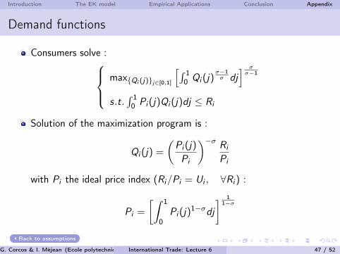
Consumers solve :max{Qi (j)}j∈[0,1]

[∫ 10 Qi (j)

σ−1σ dj

] σσ−1

s.t.∫ 10 Pi (j)Qi (j)dj ≤ Ri

Solution of the maximization program is :

Qi (j) =

(Pi (j)

Pi

)−σ Ri

Pi

with Pi the ideal price index (Ri/Pi = Ui , ∀Ri ) :

Pi =

[∫ 1

0Pi (j)

1−σdj

] 11−σ

Back to assumptions



Optimal Prices

Firms’ profit :

πi (j) =∑n

[pni (j)Qni (j)−

cizi (j)

dniQni (j)

]=∑n

πni (j)

Under perfect competition :

pni (j) =ci

zi (j)dni

andQin(j) = 0 if pin(j) > pn(j)/Qn(j) otherwise

Back to assumptions



Price distribution

pni (j) = cizi (j)

dni is the realization of a random variable Pni which cdfis :

Gni (p) = Pr [Pni ≤ p] = Pr

[Zi ≥

cidnip

]= 1− Fi

(cidnip

)= 1− e

−Ti

(ci dnip

)−θ

pn(j) = min{pni (j); i = 1...I} is the realization of a random variablePn = min{Pni ; i = 1...I} which cdf is :

Gn(p) = Pr [Pn ≤ p] = 1−I∏

i=1

Pr [Pni > p]

= 1−I∏

i=1

[1− Gni (p)] = 1− e−pθ∑I

i=1 Ti (cidni )−θ

Back to the model



Price index

Cdf / pdf of consumption prices :

Fn(p) = 1− e−Φnpθ

and fn(p) = Φnθpθ−1e−Φnp

θ

Define : y = g(p) = pθ, then

Gn(y) = Fn(g−1(y)) and gn(y) = f (g−1(y))

∣∣∣∣∂g−1(y)

∂y

∣∣∣∣ = Φne−Φny

Thus the price index :

Pn =

[∫ 1

0pn(j)1−σdj

] 11−σ

=

[∫ 1

0y

1−σθ Φne

−Φnydy

] 11−σ

= Φ−1/θn

[∫ 1

0u

1−σθ e−udu

] 11−σ

where u = Φny

= Φ−1/θn

[Γ

(1− σθ− 1)] 1

1−σ

Back to the modelG. Corcos & I. Méjean (Ecole polytechnique) International Trade: Lecture 6 50 / 52


Fréchet distribution

Generalized extreme value distribution : A family of continuousprobability distributions used as an approximation to model themaxima of long (finite) sequences of random variablesCDF :

F (x ;µ, σ, ξ) = exp

{−[1 + ξ

(x − µσ

)]− 1ξ

}µ a location parameter, σ > 0 the scale parameter, ξ the shapeparameter



Fréchet distribution

In particular :I Gumbel or type I extreme value : ξ = 0

F (x ;µ, σ, 0) = exp

{−exp

[−x − µ

σ

]}, x ∈ R

I Frechet of type II extreme value : ξ = α−1 > 0

F (x ;µ, σ, ξ) =

{0, x ≤ µexp

{−[x−µσ

]−α}, x > µ

I Reversed Weibull or type III extreme value : ξ = −α−1 < 0

F (x ;µ, σ, ξ) =

{exp

{−[− x−µ

σ

]α}, x < µ

1, x ≥ µ

Back to the model


Lecture 6: Technology, Geography and Tradegregory.corcos.free.fr/M2/lecture 6.pdf ·...

Documents

Transcript of Lecture 6: Technology, Geography and Tradegregory.corcos.free.fr/M2/lecture 6.pdf ·...