Lecture 6 Optimization for Deep Neural Networks - CMSC...
179
Lecture 6 Optimization for Deep Neural Networks CMSC 35246: Deep Learning Shubhendu Trivedi & Risi Kondor University of Chicago April 12, 2017 Lecture 6 Optimization for Deep Neural Networks CMSC 35246
Transcript of Lecture 6 Optimization for Deep Neural Networks - CMSC...

Lecture 6Optimization for Deep Neural Networks
CMSC 35246: Deep Learning
Shubhendu Trivedi&
Risi Kondor
University of Chicago
April 12, 2017
Lecture 6 Optimization for Deep Neural Networks CMSC 35246

Things we will look at today
• Stochastic Gradient Descent
• Momentum Method and the Nesterov Variant• Adaptive Learning Methods (AdaGrad, RMSProp, Adam)• Batch Normalization• Intialization Heuristics• Polyak Averaging• On Slides but for self study: Newton and Quasi Newton
Methods (BFGS, L-BFGS, Conjugate Gradient)
Lecture 6 Optimization for Deep Neural Networks CMSC 35246
Things we will look at today
• Stochastic Gradient Descent• Momentum Method and the Nesterov Variant
• Adaptive Learning Methods (AdaGrad, RMSProp, Adam)• Batch Normalization• Intialization Heuristics• Polyak Averaging• On Slides but for self study: Newton and Quasi Newton
Methods (BFGS, L-BFGS, Conjugate Gradient)
Lecture 6 Optimization for Deep Neural Networks CMSC 35246

Things we will look at today
• Stochastic Gradient Descent• Momentum Method and the Nesterov Variant• Adaptive Learning Methods (AdaGrad, RMSProp, Adam)
• Batch Normalization• Intialization Heuristics• Polyak Averaging• On Slides but for self study: Newton and Quasi Newton
Methods (BFGS, L-BFGS, Conjugate Gradient)
Lecture 6 Optimization for Deep Neural Networks CMSC 35246

Things we will look at today
• Stochastic Gradient Descent• Momentum Method and the Nesterov Variant• Adaptive Learning Methods (AdaGrad, RMSProp, Adam)• Batch Normalization
• Intialization Heuristics• Polyak Averaging• On Slides but for self study: Newton and Quasi Newton
Methods (BFGS, L-BFGS, Conjugate Gradient)
Lecture 6 Optimization for Deep Neural Networks CMSC 35246

Things we will look at today
• Stochastic Gradient Descent• Momentum Method and the Nesterov Variant• Adaptive Learning Methods (AdaGrad, RMSProp, Adam)• Batch Normalization• Intialization Heuristics
• Polyak Averaging• On Slides but for self study: Newton and Quasi Newton
Methods (BFGS, L-BFGS, Conjugate Gradient)
Lecture 6 Optimization for Deep Neural Networks CMSC 35246

Things we will look at today
• Stochastic Gradient Descent• Momentum Method and the Nesterov Variant• Adaptive Learning Methods (AdaGrad, RMSProp, Adam)• Batch Normalization• Intialization Heuristics• Polyak Averaging
• On Slides but for self study: Newton and Quasi NewtonMethods (BFGS, L-BFGS, Conjugate Gradient)
Lecture 6 Optimization for Deep Neural Networks CMSC 35246

Things we will look at today
• Stochastic Gradient Descent• Momentum Method and the Nesterov Variant• Adaptive Learning Methods (AdaGrad, RMSProp, Adam)• Batch Normalization• Intialization Heuristics• Polyak Averaging• On Slides but for self study: Newton and Quasi Newton
Methods (BFGS, L-BFGS, Conjugate Gradient)
Lecture 6 Optimization for Deep Neural Networks CMSC 35246

Optimization
We’ve seen backpropagation as a method for computinggradients
Assignment: Was about implementation of SGD inconjunction with backprop
Let’s see a family of first order methods
Lecture 6 Optimization for Deep Neural Networks CMSC 35246

Optimization
We’ve seen backpropagation as a method for computinggradients
Assignment: Was about implementation of SGD inconjunction with backprop
Let’s see a family of first order methods
Lecture 6 Optimization for Deep Neural Networks CMSC 35246

Optimization
We’ve seen backpropagation as a method for computinggradients
Assignment: Was about implementation of SGD inconjunction with backprop
Let’s see a family of first order methods
Lecture 6 Optimization for Deep Neural Networks CMSC 35246

Batch Gradient Descent
Algorithm 1 Batch Gradient Descent at Iteration k
Require: Learning rate εkRequire: Initial Parameter θ1: while stopping criteria not met do2: Compute gradient estimate over N examples:3: g← + 1
N∇θ∑
i L(f(x(i); θ),y(i))4: Apply Update: θ ← θ − εg5: end while
Positive: Gradient estimates are stable
Negative: Need to compute gradients over the entire trainingfor one update
Lecture 6 Optimization for Deep Neural Networks CMSC 35246

Gradient Descent
Lecture 6 Optimization for Deep Neural Networks CMSC 35246

Gradient Descent
Lecture 6 Optimization for Deep Neural Networks CMSC 35246

Gradient Descent
Lecture 6 Optimization for Deep Neural Networks CMSC 35246

Gradient Descent
Lecture 6 Optimization for Deep Neural Networks CMSC 35246

Gradient Descent
Lecture 6 Optimization for Deep Neural Networks CMSC 35246

Gradient Descent
Lecture 6 Optimization for Deep Neural Networks CMSC 35246
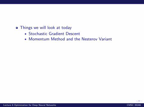
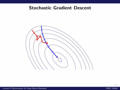
Stochastic Gradient Descent
Algorithm 2 Stochastic Gradient Descent at Iteration k
Require: Learning rate εkRequire: Initial Parameter θ1: while stopping criteria not met do2: Sample example (x(i),y(i)) from training set3: Compute gradient estimate:4: g← +∇θL(f(x(i); θ),y(i))5: Apply Update: θ ← θ − εg6: end while
εk is learning rate at step kSufficient condition to guarantee convergence:
∞∑k=1
εk =∞ and∞∑k=1
ε2k <∞
Lecture 6 Optimization for Deep Neural Networks CMSC 35246

Stochastic Gradient Descent
Algorithm 2 Stochastic Gradient Descent at Iteration k
Require: Learning rate εkRequire: Initial Parameter θ1: while stopping criteria not met do2: Sample example (x(i),y(i)) from training set3: Compute gradient estimate:4: g← +∇θL(f(x(i); θ),y(i))5: Apply Update: θ ← θ − εg6: end while
εk is learning rate at step k
Sufficient condition to guarantee convergence:∞∑k=1
εk =∞ and∞∑k=1
ε2k <∞
Lecture 6 Optimization for Deep Neural Networks CMSC 35246

Stochastic Gradient Descent
Algorithm 2 Stochastic Gradient Descent at Iteration k
Require: Learning rate εkRequire: Initial Parameter θ1: while stopping criteria not met do2: Sample example (x(i),y(i)) from training set3: Compute gradient estimate:4: g← +∇θL(f(x(i); θ),y(i))5: Apply Update: θ ← θ − εg6: end while
εk is learning rate at step kSufficient condition to guarantee convergence:
∞∑k=1
εk =∞ and∞∑k=1
ε2k <∞
Lecture 6 Optimization for Deep Neural Networks CMSC 35246

Learning Rate Schedule
In practice the learning rate is decayed linearly till iteration τ
εk = (1− α)ε0 + αετ with α =k
τ
τ is usually set to the number of iterations needed for a largenumber of passes through the data
ετ should roughly be set to 1% of ε0
How to set ε0?
Lecture 6 Optimization for Deep Neural Networks CMSC 35246

Minibatching
Potential Problem: Gradient estimates can be very noisy
Obvious Solution: Use larger mini-batches
Advantage: Computation time per update does not depend onnumber of training examples N
This allows convergence on extremely large datasets
See: Large Scale Learning with Stochastic Gradient Descentby Leon Bottou
Lecture 6 Optimization for Deep Neural Networks CMSC 35246

Stochastic Gradient Descent
Lecture 6 Optimization for Deep Neural Networks CMSC 35246

Stochastic Gradient Descent
Lecture 6 Optimization for Deep Neural Networks CMSC 35246
Stochastic Gradient Descent
Lecture 6 Optimization for Deep Neural Networks CMSC 35246

Stochastic Gradient Descent
Lecture 6 Optimization for Deep Neural Networks CMSC 35246

Stochastic Gradient Descent
Lecture 6 Optimization for Deep Neural Networks CMSC 35246

Stochastic Gradient Descent
Lecture 6 Optimization for Deep Neural Networks CMSC 35246

Stochastic Gradient Descent
Lecture 6 Optimization for Deep Neural Networks CMSC 35246

Stochastic Gradient Descent
Lecture 6 Optimization for Deep Neural Networks CMSC 35246

Stochastic Gradient Descent
Lecture 6 Optimization for Deep Neural Networks CMSC 35246

So far..
Batch Gradient Descent:
g← +1
N∇θ∑i
L(f(x(i); θ),y(i))
θ ← θ − εg
SGD:
g← +∇θL(f(x(i); θ),y(i))
θ ← θ − εg
Lecture 6 Optimization for Deep Neural Networks CMSC 35246

So far..
Batch Gradient Descent:
g← +1
N∇θ∑i
L(f(x(i); θ),y(i))
θ ← θ − εg
SGD:
g← +∇θL(f(x(i); θ),y(i))
θ ← θ − εg
Lecture 6 Optimization for Deep Neural Networks CMSC 35246

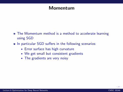
Momentum
The Momentum method is a method to accelerate learningusing SGD
In particular SGD suffers in the following scenarios:
• Error surface has high curvature• We get small but consistent gradients• The gradients are very noisy
Lecture 6 Optimization for Deep Neural Networks CMSC 35246

Momentum
The Momentum method is a method to accelerate learningusing SGD
In particular SGD suffers in the following scenarios:
• Error surface has high curvature
• We get small but consistent gradients• The gradients are very noisy
Lecture 6 Optimization for Deep Neural Networks CMSC 35246

Momentum
The Momentum method is a method to accelerate learningusing SGD
In particular SGD suffers in the following scenarios:
• Error surface has high curvature• We get small but consistent gradients
• The gradients are very noisy
Lecture 6 Optimization for Deep Neural Networks CMSC 35246
Momentum
The Momentum method is a method to accelerate learningusing SGD
In particular SGD suffers in the following scenarios:
• Error surface has high curvature• We get small but consistent gradients• The gradients are very noisy
Lecture 6 Optimization for Deep Neural Networks CMSC 35246

Momentum
−4 −2 02
4 −5
0
5
0
500
1.000
Gradient Descent would move quickly down the walls, butvery slowly through the valley floor
Lecture 6 Optimization for Deep Neural Networks CMSC 35246

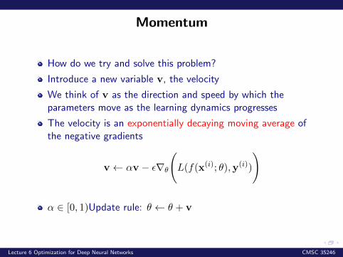
Momentum
How do we try and solve this problem?
Introduce a new variable v, the velocity
We think of v as the direction and speed by which theparameters move as the learning dynamics progresses
The velocity is an exponentially decaying moving average ofthe negative gradients
v← αv − ε∇θ
(L(f(x(i); θ),y(i))
)
α ∈ [0, 1)Update rule: θ ← θ + v
Lecture 6 Optimization for Deep Neural Networks CMSC 35246

Momentum
Let’s look at the velocity term:
v← αv − ε∇θ
(L(f(x(i); θ),y(i))
)
The velocity accumulates the previous gradients
What is the role of α?
• If α is larger than ε the current update is more affectedby the previous gradients
• Usually values for α are set high ≈ 0.8, 0.9
Lecture 6 Optimization for Deep Neural Networks CMSC 35246

Momentum
Gradient Step
Momentum Step Actual Step
Lecture 6 Optimization for Deep Neural Networks CMSC 35246

Momentum
Gradient Step
Momentum Step
Actual Step
Lecture 6 Optimization for Deep Neural Networks CMSC 35246

Momentum
Gradient Step
Momentum Step Actual Step
Lecture 6 Optimization for Deep Neural Networks CMSC 35246

Momentum: Step Sizes
In SGD, the step size was the norm of the gradient scaled bythe learning rate ε‖g‖. Why?
While using momentum, the step size will also depend on thenorm and alignment of a sequence of gradients
For example, if at each step we observed g, the step sizewould be (exercise!):
ε‖g‖
1− α
If α = 0.9 =⇒ multiply the maximum speed by 10 relative tothe current gradient direction
Lecture 6 Optimization for Deep Neural Networks CMSC 35246

Momentum
Illustration of how momentum traverses such an error surfacebetter compared to Gradient Descent
Lecture 6 Optimization for Deep Neural Networks CMSC 35246
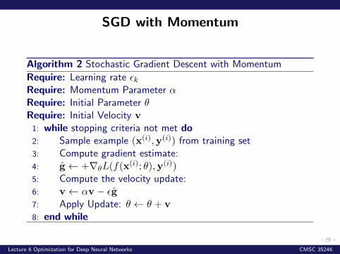
SGD with Momentum
Algorithm 2 Stochastic Gradient Descent with Momentum
Require: Learning rate εkRequire: Momentum Parameter αRequire: Initial Parameter θRequire: Initial Velocity v1: while stopping criteria not met do2: Sample example (x(i),y(i)) from training set3: Compute gradient estimate:4: g← +∇θL(f(x(i); θ),y(i))5: Compute the velocity update:6: v← αv − εg7: Apply Update: θ ← θ + v8: end while
Lecture 6 Optimization for Deep Neural Networks CMSC 35246

Nesterov Momentum
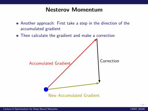
Another approach: First take a step in the direction of theaccumulated gradient
Then calculate the gradient and make a correction
Accumulated Gradient
Correction
New Accumulated Gradient
Lecture 6 Optimization for Deep Neural Networks CMSC 35246

Nesterov Momentum
Another approach: First take a step in the direction of theaccumulated gradient
Then calculate the gradient and make a correction
Accumulated GradientCorrection
New Accumulated Gradient
Lecture 6 Optimization for Deep Neural Networks CMSC 35246
Nesterov Momentum
Another approach: First take a step in the direction of theaccumulated gradient
Then calculate the gradient and make a correction
Accumulated GradientCorrection
New Accumulated Gradient
Lecture 6 Optimization for Deep Neural Networks CMSC 35246

Nesterov Momentum
Next Step
Lecture 6 Optimization for Deep Neural Networks CMSC 35246

Nesterov Momentum
Next Step
Lecture 6 Optimization for Deep Neural Networks CMSC 35246

Nesterov Momentum
Next Step
Lecture 6 Optimization for Deep Neural Networks CMSC 35246

Nesterov Momentum
Next Step
Lecture 6 Optimization for Deep Neural Networks CMSC 35246

Let’s Write it out..
Recall the velocity term in the Momentum method:
v← αv − ε∇θ
(L(f(x(i); θ),y(i))
)
Nesterov Momentum:
v← αv − ε∇θ
(L(f(x(i); θ + αv),y(i))
)
Update: θ ← θ + v
Lecture 6 Optimization for Deep Neural Networks CMSC 35246

Let’s Write it out..
Recall the velocity term in the Momentum method:
v← αv − ε∇θ
(L(f(x(i); θ),y(i))
)
Nesterov Momentum:
v← αv − ε∇θ
(L(f(x(i); θ + αv),y(i))
)
Update: θ ← θ + v
Lecture 6 Optimization for Deep Neural Networks CMSC 35246

Let’s Write it out..
Recall the velocity term in the Momentum method:
v← αv − ε∇θ
(L(f(x(i); θ),y(i))
)
Nesterov Momentum:
v← αv − ε∇θ
(L(f(x(i); θ + αv),y(i))
)
Update: θ ← θ + v
Lecture 6 Optimization for Deep Neural Networks CMSC 35246

SGD with Nesterov Momentum
Algorithm 3 SGD with Nesterov Momentum
Require: Learning rate εRequire: Momentum Parameter αRequire: Initial Parameter θRequire: Initial Velocity v1: while stopping criteria not met do2: Sample example (x(i),y(i)) from training set3: Update parameters: θ ← θ + αv4: Compute gradient estimate:5: g← +∇θL(f(x(i); θ),y(i))6: Compute the velocity update: v← αv − εg7: Apply Update: θ ← θ + v8: end while
Lecture 6 Optimization for Deep Neural Networks CMSC 35246

Adaptive Learning Rate Methods
Lecture 6 Optimization for Deep Neural Networks CMSC 35246

Motivation
Till now we assign the same learning rate to all features
If the features vary in importance and frequency, why is this agood idea?
It’s probably not!
Lecture 6 Optimization for Deep Neural Networks CMSC 35246

Motivation
Till now we assign the same learning rate to all features
If the features vary in importance and frequency, why is this agood idea?
It’s probably not!
Lecture 6 Optimization for Deep Neural Networks CMSC 35246

Motivation
Till now we assign the same learning rate to all features
If the features vary in importance and frequency, why is this agood idea?
It’s probably not!
Lecture 6 Optimization for Deep Neural Networks CMSC 35246

Motivation
Nice (all features are equally important)
Lecture 6 Optimization for Deep Neural Networks CMSC 35246
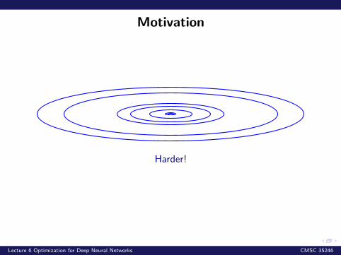
Motivation
Harder!
Lecture 6 Optimization for Deep Neural Networks CMSC 35246

AdaGrad
Idea: Downscale a model parameter by square-root of sum ofsquares of all its historical values
Parameters that have large partial derivative of the loss –learning rates for them are rapidly declined
Some interesting theoretical properties
Lecture 6 Optimization for Deep Neural Networks CMSC 35246

AdaGrad
Algorithm 4 AdaGrad
Require: Global Learning rate ε, Initial Parameter θ, δInitialize r = 01: while stopping criteria not met do2: Sample example (x(i),y(i)) from training set3: Compute gradient estimate: g← +∇θL(f(x(i); θ),y(i))4: Accumulate: r← r + g � g5: Compute update: ∆θ ← − ε
δ+√r� g
6: Apply Update: θ ← θ + ∆θ7: end while
Lecture 6 Optimization for Deep Neural Networks CMSC 35246

RMSProp
AdaGrad is good when the objective is convex.
AdaGrad might shrink the learning rate too aggressively, wewant to keep the history in mind
We can adapt it to perform better in non-convex settings byaccumulating an exponentially decaying average of thegradient
This is an idea that we use again and again in NeuralNetworks
Currently has about 500 citations on scholar, but wasproposed in a slide in Geoffrey Hinton’s coursera course
Lecture 6 Optimization for Deep Neural Networks CMSC 35246

RMSProp
Algorithm 5 RMSProp
Require: Global Learning rate ε, decay parameter ρ, δInitialize r = 01: while stopping criteria not met do2: Sample example (x(i),y(i)) from training set3: Compute gradient estimate: g← +∇θL(f(x(i); θ),y(i))4: Accumulate: r← ρr + (1− ρ)g � g5: Compute update: ∆θ ← − ε
δ+√r� g
6: Apply Update: θ ← θ + ∆θ7: end while
Lecture 6 Optimization for Deep Neural Networks CMSC 35246

RMSProp with Nesterov
Algorithm 6 RMSProp with Nesterov
Require: Global Learning rate ε, decay parameter ρ, δ, α, vInitialize r = 01: while stopping criteria not met do2: Sample example (x(i),y(i)) from training set3: Compute Update: θ ← θ + αv4: Compute gradient estimate: g← +∇θL(f(x(i); θ),y(i))5: Accumulate: r← ρr + (1− ρ)g � g6: Compute Velocity: v← αv − ε√
r� g
7: Apply Update: θ ← θ + v8: end while
Lecture 6 Optimization for Deep Neural Networks CMSC 35246
Adam
We could have used RMSProp with momentum
Use of Momentum with rescaling is not well motivated
Adam is like RMSProp with Momentum but with biascorrection terms for the first and second moments
Lecture 6 Optimization for Deep Neural Networks CMSC 35246

Adam
We could have used RMSProp with momentum
Use of Momentum with rescaling is not well motivated
Adam is like RMSProp with Momentum but with biascorrection terms for the first and second moments
Lecture 6 Optimization for Deep Neural Networks CMSC 35246
Adam
We could have used RMSProp with momentum
Use of Momentum with rescaling is not well motivated
Adam is like RMSProp with Momentum but with biascorrection terms for the first and second moments
Lecture 6 Optimization for Deep Neural Networks CMSC 35246

Adam: ADAptive Moments
Algorithm 7 RMSProp with Nesterov
Require: ε (set to 0.0001), decay rates ρ1 (set to 0.9), ρ2 (set to0.9), θ, δInitialize moments variables s = 0 and r = 0, time step t = 01: while stopping criteria not met do2: Sample example (x(i),y(i)) from training set3: Compute gradient estimate: g← +∇θL(f(x(i); θ),y(i))4: t← t+ 15: Update: s← ρ1s + (1− ρ1)g6: Update: r← ρ2r + (1− ρ2)g � g7: Correct Biases: s← s
1−ρt1, r← r
1−ρt28: Compute Update: ∆θ = −ε s√
r+δ9: Apply Update: θ ← θ + ∆θ
10: end while
Lecture 6 Optimization for Deep Neural Networks CMSC 35246

All your GRADs are belong to us!
SGD: θ ← θ − εgMomentum: v← αv − εg then θ ← θ + v
Nesterov: v← αv − ε∇θ
(L(f(x(i); θ + αv),y(i))
)then θ ← θ + v
AdaGrad: r← r + g � g then ∆θ− ← ε
δ +√r� g then θ ← θ + ∆θ
RMSProp: r← ρr + (1− ρ)g � g then ∆θ ← − ε
δ +√r� g then θ ← θ + ∆θ
Adam: s← s
1− ρt1, r← r
1− ρt2then ∆θ = −ε s√
r + δthen θ ← θ + ∆θ
Lecture 6 Optimization for Deep Neural Networks CMSC 35246

Batch Normalization
Lecture 6 Optimization for Deep Neural Networks CMSC 35246

A Difficulty in Training Deep Neural Networks
A deep model involves composition of several functionsy = W T
4 (tanh(W T3 (tanh(W T
2 (tanh(W T1 x + b1) + b2) + b3))))
x1 x2 x3 x4
y
Lecture 6 Optimization for Deep Neural Networks CMSC 35246

A Difficulty in Training Deep Neural Networks
We have a recipe to compute gradients (Backpropagation),and update every parameter (we saw half a dozen methods)
Implicit Assumption: Other layers don’t change i.e. otherfunctions are fixed
In Practice: We update all layers simultaneously
This can give rise to unexpected difficulties
Let’s look at two illustrations
Lecture 6 Optimization for Deep Neural Networks CMSC 35246

Intuition
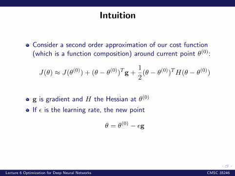
Consider a second order approximation of our cost function(which is a function composition) around current point θ(0):
J(θ) ≈ J(θ(0)) + (θ − θ(0))Tg +1
2(θ − θ(0))TH(θ − θ(0))
g is gradient and H the Hessian at θ(0)
If ε is the learning rate, the new point
θ = θ(0) − εg
Lecture 6 Optimization for Deep Neural Networks CMSC 35246

Intuition
Consider a second order approximation of our cost function(which is a function composition) around current point θ(0):
J(θ) ≈ J(θ(0)) + (θ − θ(0))Tg +1
2(θ − θ(0))TH(θ − θ(0))
g is gradient and H the Hessian at θ(0)
If ε is the learning rate, the new point
θ = θ(0) − εg
Lecture 6 Optimization for Deep Neural Networks CMSC 35246

Intuition
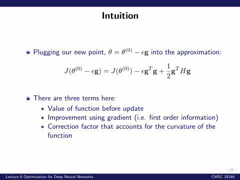
Plugging our new point, θ = θ(0) − εg into the approximation:
J(θ(0) − εg) = J(θ(0))− εgTg +1
2gTHg
There are three terms here:
• Value of function before update• Improvement using gradient (i.e. first order information)• Correction factor that accounts for the curvature of the
function
Lecture 6 Optimization for Deep Neural Networks CMSC 35246

Intuition
Plugging our new point, θ = θ(0) − εg into the approximation:
J(θ(0) − εg) = J(θ(0))− εgTg +1
2gTHg
There are three terms here:
• Value of function before update
• Improvement using gradient (i.e. first order information)• Correction factor that accounts for the curvature of the
function
Lecture 6 Optimization for Deep Neural Networks CMSC 35246

Intuition
Plugging our new point, θ = θ(0) − εg into the approximation:
J(θ(0) − εg) = J(θ(0))− εgTg +1
2gTHg
There are three terms here:
• Value of function before update• Improvement using gradient (i.e. first order information)
• Correction factor that accounts for the curvature of thefunction
Lecture 6 Optimization for Deep Neural Networks CMSC 35246
Intuition
Plugging our new point, θ = θ(0) − εg into the approximation:
J(θ(0) − εg) = J(θ(0))− εgTg +1
2gTHg
There are three terms here:
• Value of function before update• Improvement using gradient (i.e. first order information)• Correction factor that accounts for the curvature of the
function
Lecture 6 Optimization for Deep Neural Networks CMSC 35246

Intuition
J(θ(0) − εg) = J(θ(0))− εgTg +1
2gTHg
Observations:
• gTHg too large: Gradient will start moving upwards• gTHg = 0: J will decrease for even large ε• Optimal step size ε∗ = gTg for zero curvature,
ε∗ = gT ggTHg
to take into account curvature
Conclusion: Just neglecting second order effects can causeproblems (remedy: second order methods). What abouthigher order effects?
Lecture 6 Optimization for Deep Neural Networks CMSC 35246

Intuition
J(θ(0) − εg) = J(θ(0))− εgTg +1
2gTHg
Observations:
• gTHg too large: Gradient will start moving upwards
• gTHg = 0: J will decrease for even large ε• Optimal step size ε∗ = gTg for zero curvature,
ε∗ = gT ggTHg
to take into account curvature
Conclusion: Just neglecting second order effects can causeproblems (remedy: second order methods). What abouthigher order effects?
Lecture 6 Optimization for Deep Neural Networks CMSC 35246

Intuition
J(θ(0) − εg) = J(θ(0))− εgTg +1
2gTHg
Observations:
• gTHg too large: Gradient will start moving upwards• gTHg = 0: J will decrease for even large ε
• Optimal step size ε∗ = gTg for zero curvature,
ε∗ = gT ggTHg
to take into account curvature
Conclusion: Just neglecting second order effects can causeproblems (remedy: second order methods). What abouthigher order effects?
Lecture 6 Optimization for Deep Neural Networks CMSC 35246

Intuition
J(θ(0) − εg) = J(θ(0))− εgTg +1
2gTHg
Observations:
• gTHg too large: Gradient will start moving upwards• gTHg = 0: J will decrease for even large ε• Optimal step size ε∗ = gTg for zero curvature,
ε∗ = gT ggTHg
to take into account curvature
Conclusion: Just neglecting second order effects can causeproblems (remedy: second order methods). What abouthigher order effects?
Lecture 6 Optimization for Deep Neural Networks CMSC 35246

Intuition
J(θ(0) − εg) = J(θ(0))− εgTg +1
2gTHg
Observations:
• gTHg too large: Gradient will start moving upwards• gTHg = 0: J will decrease for even large ε• Optimal step size ε∗ = gTg for zero curvature,
ε∗ = gT ggTHg
to take into account curvature
Conclusion: Just neglecting second order effects can causeproblems (remedy: second order methods). What abouthigher order effects?
Lecture 6 Optimization for Deep Neural Networks CMSC 35246

Higher Order Effects: Toy Model
x
h1
h2
...hl
y
w1
w2
wl
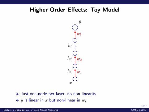
Just one node per layer, no non-linearity
y is linear in x but non-linear in wi
Lecture 6 Optimization for Deep Neural Networks CMSC 35246

Higher Order Effects: Toy Model
x
h1
h2
...hl
y
w1
w2
wl
Just one node per layer, no non-linearity
y is linear in x but non-linear in wi
Lecture 6 Optimization for Deep Neural Networks CMSC 35246
Higher Order Effects: Toy Model
x
h1
h2
...hl
y
w1
w2
wl
Just one node per layer, no non-linearity
y is linear in x but non-linear in wi
Lecture 6 Optimization for Deep Neural Networks CMSC 35246

Higher Order Effects: Toy Model
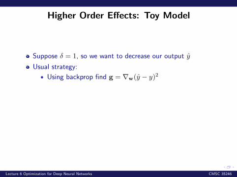
Suppose δ = 1, so we want to decrease our output y
Usual strategy:
• Using backprop find g = ∇w(y − y)2
• Update weights w := w − εgThe first order Taylor approximation (in previous slide) saysthe cost will reduce by εgTg
If we need to reduce cost by 0.1, then learning rate should be0.1gT g
Lecture 6 Optimization for Deep Neural Networks CMSC 35246
Higher Order Effects: Toy Model
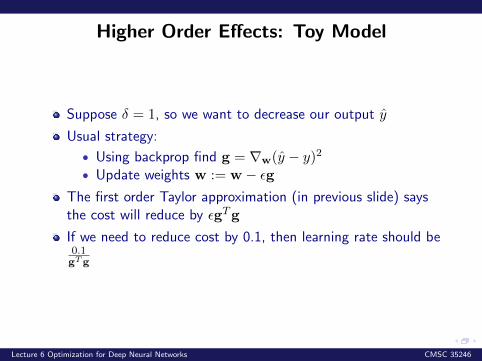
Suppose δ = 1, so we want to decrease our output y
Usual strategy:
• Using backprop find g = ∇w(y − y)2
• Update weights w := w − εgThe first order Taylor approximation (in previous slide) saysthe cost will reduce by εgTg
If we need to reduce cost by 0.1, then learning rate should be0.1gT g
Lecture 6 Optimization for Deep Neural Networks CMSC 35246

Higher Order Effects: Toy Model
Suppose δ = 1, so we want to decrease our output y
Usual strategy:
• Using backprop find g = ∇w(y − y)2
• Update weights w := w − εg
The first order Taylor approximation (in previous slide) saysthe cost will reduce by εgTg
If we need to reduce cost by 0.1, then learning rate should be0.1gT g
Lecture 6 Optimization for Deep Neural Networks CMSC 35246

Higher Order Effects: Toy Model
Suppose δ = 1, so we want to decrease our output y
Usual strategy:
• Using backprop find g = ∇w(y − y)2
• Update weights w := w − εgThe first order Taylor approximation (in previous slide) saysthe cost will reduce by εgTg
If we need to reduce cost by 0.1, then learning rate should be0.1gT g
Lecture 6 Optimization for Deep Neural Networks CMSC 35246

Higher Order Effects: Toy Model
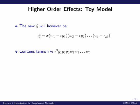
The new y will however be:
y = x(w1 − εg1)(w2 − εg2) . . . (wl − εgl)
Contains terms like ε3g1g2g3w4w5 . . . wl
If weights w4, w5, . . . , wl are small, the term is negligible. Butif large, it would explode
Conclusion: Higher order terms make it very hard to choosethe right learning rate
Second Order Methods are already expensive, nth ordermethods are hopeless. Solution?
Lecture 6 Optimization for Deep Neural Networks CMSC 35246
Higher Order Effects: Toy Model
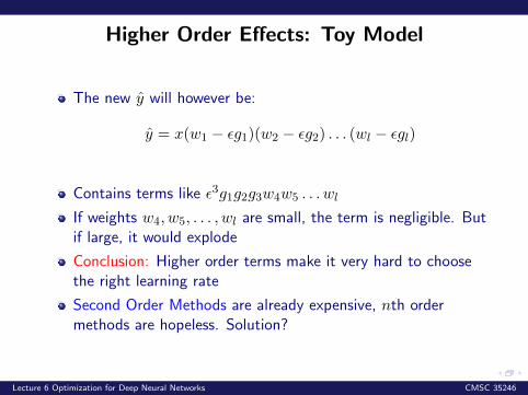
The new y will however be:
y = x(w1 − εg1)(w2 − εg2) . . . (wl − εgl)
Contains terms like ε3g1g2g3w4w5 . . . wl
If weights w4, w5, . . . , wl are small, the term is negligible. Butif large, it would explode
Conclusion: Higher order terms make it very hard to choosethe right learning rate
Second Order Methods are already expensive, nth ordermethods are hopeless. Solution?
Lecture 6 Optimization for Deep Neural Networks CMSC 35246

Higher Order Effects: Toy Model
The new y will however be:
y = x(w1 − εg1)(w2 − εg2) . . . (wl − εgl)
Contains terms like ε3g1g2g3w4w5 . . . wl
If weights w4, w5, . . . , wl are small, the term is negligible. Butif large, it would explode
Conclusion: Higher order terms make it very hard to choosethe right learning rate
Second Order Methods are already expensive, nth ordermethods are hopeless. Solution?
Lecture 6 Optimization for Deep Neural Networks CMSC 35246

Batch Normalization
Method to reparameterize a deep network to reduceco-ordination of update across layers
Can be applied to input layer, or any hidden layer
Let H be a design matrix having activations in any layer form examples in the mini-batch
H =
h11 h12 h13 . . . h1kh21 h22 h23 . . . h2k
......
.... . .
...
hm1 hm2 hm3 . . . hmk
Lecture 6 Optimization for Deep Neural Networks CMSC 35246

Batch Normalization
H =
h11 h12 h13 . . . h1kh21 h22 h23 . . . h2k
......
.... . .
...
hm1 hm2 hm3 . . . hmk
Each row represents all the activations in layer for one example
Idea: Replace H by H ′ such that:
H ′ =H − µσ
µ is mean of each unit and σ the standard deviation
Lecture 6 Optimization for Deep Neural Networks CMSC 35246

Batch Normalization
µ is a vector with µj the column mean
σ is a vector with σj the column standard deviation
Hi,j is normalized by subtracting µj and dividing by σj
Lecture 6 Optimization for Deep Neural Networks CMSC 35246

Batch Normalization
µ is a vector with µj the column mean
σ is a vector with σj the column standard deviation
Hi,j is normalized by subtracting µj and dividing by σj
Lecture 6 Optimization for Deep Neural Networks CMSC 35246

Batch Normalization
µ is a vector with µj the column mean
σ is a vector with σj the column standard deviation
Hi,j is normalized by subtracting µj and dividing by σj
Lecture 6 Optimization for Deep Neural Networks CMSC 35246

Batch Normalization
During training we have:
µ =1
m
∑j
H:,j
σ =
√δ +
1
m
∑j
(H − µ)2j
We then operate on H ′ as before =⇒ we backpropagatethrough the normalized activations
Lecture 6 Optimization for Deep Neural Networks CMSC 35246

Batch Normalization
During training we have:
µ =1
m
∑j
H:,j
σ =
√δ +
1
m
∑j
(H − µ)2j
We then operate on H ′ as before =⇒ we backpropagatethrough the normalized activations
Lecture 6 Optimization for Deep Neural Networks CMSC 35246

Why is this good?
The update will never act to only increase the mean andstandard deviation of any activation
Previous approaches added penalties to cost or per layer toencourage units to have standardized outputs
Batch normalization makes the reparameterization easier
At test time: Use running averages of µ and σ collectedduring training, use these for evaluating new input x
Lecture 6 Optimization for Deep Neural Networks CMSC 35246

An Innovation
Standardizing the output of a unit can limit the expressivepower of the neural network
Solution: Instead of replacing H by H ′, replace it will γH ′+β
γ and β are also learned by backpropagation
Normalizing for mean and standard deviation was the goal ofbatch normalization, why add γ and β again?
Lecture 6 Optimization for Deep Neural Networks CMSC 35246

Initialization Strategies
Lecture 6 Optimization for Deep Neural Networks CMSC 35246

In convex problems with good ε no matter what theinitialization, convergence is guaranteed
In the non-convex regime initialization is much moreimportant
Some parameter initialization can be unstable, not converge
Neural Networks are not well understood to have principled,mathematically nice initialization strategies
What is known: Initialization should break symmetry (quiz!)
What is known: Scale of weights is important
Most initialization strategies are based on intuitions andheuristics
Lecture 6 Optimization for Deep Neural Networks CMSC 35246

Some Heuristics
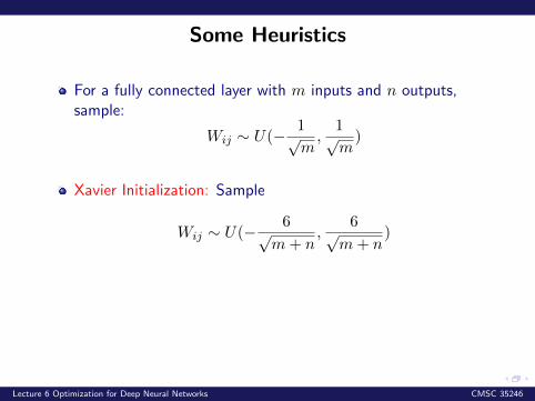
For a fully connected layer with m inputs and n outputs,sample:
Wij ∼ U(− 1√m,
1√m
)
Xavier Initialization: Sample
Wij ∼ U(− 6√m+ n
,6√
m+ n)
Xavier initialization is derived considering that the networkconsists of matrix multiplications with no nonlinearites
Works well in practice!
Lecture 6 Optimization for Deep Neural Networks CMSC 35246
Some Heuristics
For a fully connected layer with m inputs and n outputs,sample:
Wij ∼ U(− 1√m,
1√m
)
Xavier Initialization: Sample
Wij ∼ U(− 6√m+ n
,6√
m+ n)
Xavier initialization is derived considering that the networkconsists of matrix multiplications with no nonlinearites
Works well in practice!
Lecture 6 Optimization for Deep Neural Networks CMSC 35246

More Heuristics
Saxe et al. 2013, recommend initialzing to random orthogonalmatrices, with a carefully chosen gain g that accounts fornon-linearities
If g could be divined, it could solve the vanishing andexploding gradients problem (more later)
The idea of choosing g and initializing weights accordingly isthat we want norm of activations to increase, and pass backstrong gradients
Martens 2010, suggested an initialization that was sparse:Each unit could only receive k non-zero weights
Motivation: Ir is a bad idea to have all initial weights to havethe same standard deviation 1√
m
Lecture 6 Optimization for Deep Neural Networks CMSC 35246

Polyak Averaging: Motivation
Gradient points towards right
Consider gradient descent above with high step size ε
Lecture 6 Optimization for Deep Neural Networks CMSC 35246

Polyak Averaging: Motivation
Gradient points towards left
Lecture 6 Optimization for Deep Neural Networks CMSC 35246

Polyak Averaging: Motivation
Gradient points towards right
Lecture 6 Optimization for Deep Neural Networks CMSC 35246

Polyak Averaging: Motivation
Gradient points towards left
Lecture 6 Optimization for Deep Neural Networks CMSC 35246

Polyak Averaging: Motivation
Gradient points towards right
Lecture 6 Optimization for Deep Neural Networks CMSC 35246

A Solution: Polyak Averaging
Suppose in t iterations you have parameters θ(1), θ(2), . . . , θ(t)
Polyak Averaging suggests setting θ(t) = 1t
∑i θ
(i)
Has strong convergence guarantees in convex settings
Is this a good idea in non-convex problems?
Lecture 6 Optimization for Deep Neural Networks CMSC 35246

Simple Modification
In non-convex surfaces the parameter space can differ greatlyin different regions
Averaging is not useful
Typical to consider the exponentially decaying average instead:
θ(t) = αθ(t−1) + (1− α)θ(t) with α ∈ [0, 1]
Lecture 6 Optimization for Deep Neural Networks CMSC 35246

Simple Modification
In non-convex surfaces the parameter space can differ greatlyin different regions
Averaging is not useful
Typical to consider the exponentially decaying average instead:
θ(t) = αθ(t−1) + (1− α)θ(t) with α ∈ [0, 1]
Lecture 6 Optimization for Deep Neural Networks CMSC 35246

Simple Modification
In non-convex surfaces the parameter space can differ greatlyin different regions
Averaging is not useful
Typical to consider the exponentially decaying average instead:
θ(t) = αθ(t−1) + (1− α)θ(t) with α ∈ [0, 1]
Lecture 6 Optimization for Deep Neural Networks CMSC 35246

Next time
Convolutional Neural Networks
Lecture 6 Optimization for Deep Neural Networks CMSC 35246