Lecture 6: Monte Carlo Simulation

6.0002 LECTURE 6 1

Relevant Reading

Sections 15-1 15.4 Chapter 16

6.0002 LECTURE 6 2

A Little History

Ulam, recovering from an illness, was playing a lot ofsolitaire

Tried to figure out probability of winning, and failed

Thought about playing lots of hands and countingnumber of wins, but decided it would take years

Asked Von Neumann if he could build a program tosimulate many hands on ENIAC

6.0002 LECTURE 6 3

Image of ENIAC programmers © unknown.This contentis excluded from our Creative Commons license. For moreinformation,see https://ocw.mit.edu/help/faq-fair-use/.

Monte Carlo Simulation

A method of estimating the value of an unknown quantity using the principles of inferential statistics

Inferential statistics ◦ Population: a set of examples

◦ Sample: a proper subset of a population

◦ Key fact: a random sample tends to exhibit the same properties as the population from which it is drawn

Exactly what we did with random walks

6.0002 LECTURE 6 4

An Example

Given a single coin, estimate fraction of heads you would get if you flipped the coin an infinite number of times

Consider one flip

How confident would you be about answering 1.0?

6.0002 LECTURE 6 5

Flipping a Coin Twice

Do you think that the next flip will come up heads?

6.0002 LECTURE 6 6

Flipping a Coin 100 Times

Now do you think that the next flip will come up heads?

6.0002 LECTURE 6 7

Flipping a Coin 100 Times

Do you think that the probability of the next flip coming up heads is 52/100?

Given the data, ϭϫ best estimate

But confidence

6.0002 LECTURE 6

should be low

8

Why the Difference in Confidence?

Confidence in our estimate depends upon two things Size of sample (e.g., 100 versus 2)

Variance of sample (e.g., all heads versus 52 heads)

As the variance grows, we need larger samples to have the same degree of confidence

6.0002 LECTURE 6 9

Roulette

No need to simulate, since answers obvious

Allows us to compare simulation results to actual probabilities

6.0002 LECTURE 6 10

Image of roulette wheel © unknown. All rights reserved. This content is excluded from ourCreative Commons license. For more information, see https://ocw.mit.edu/help/faq-fair-use/.

Class Definition

class FairRoulette(): def __init__(self):

self.pockets = [] for i in range(1,37):

self.pockets.append(i) self.ball = None self.pocketOdds = len(self.pockets) - 1

def spin(self): self.ball = random.choice(self.pockets)

def betPocket(self, pocket, amt): if str(pocket) == str(self.ball):

return amt*self.pocketOdds else: return -amt

def __str__(self): return 'Fair Roulette'

6.0002 LECTURE 6 11

Monte Carlo Simulation

def playRoulette(game, numSpins, pocket, bet): totPocket = 0 for i in range(numSpins):

game.spin() totPocket += game.betPocket(pocket, bet)

if toPrint: print(numSpins, 'spins of', game) print('Expected return betting', pocket, '=',\

str(100*totPocket/numSpins) + '%\n') return (totPocket/numSpins)

game = FairRoulette() for numSpins in (100, 1000000):

for i in range(3): playRoulette(game, numSpins, 2, 1, True)

6.0002 LECTURE 6 12

100 and 1M Spins of the Wheel

100 spins of Fair Roulette Expected return betting 2 = -100.0%

100 spins of Fair Roulette Expected return betting 2 = 44.0%

100 spins of Fair Roulette Expected return betting 2 = -28.0%

1000000 spins of Fair Roulette Expected return betting 2 = -0.046%

1000000 spins of Fair Roulette Expected return betting 2 = 0.602%

1000000 spins of Fair Roulette Expected return betting 2 = 0.7964%

6.0002 LECTURE 6 13

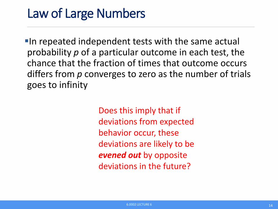
Law of Large Numbers

In repeated independent tests with the same actual probability p of a particular outcome in each test, the chance that the fraction of times that outcome occurs differs from p converges to zero as the number of trials goes to infinity

Does this imply that if deviations from expected behavior occur, these deviations are likely to be evened out by opposite deviations in the future?

6.0002 LECTURE 6 14

Gambler’s Fallacy

ϮO August 18, 1913, at the casino in Monte Carlo, black came up a record twenty-six times in succession ϭ ϿήήϨ ϩ ϴϪήή Β Β ήΒ-panicky rush to bet on red, beginning about the time black had come up a phenomenal fifteen ϭήϨϯ -- Huff and Geis, How to Take a Chance

Probability of 26 consecutive reds

1/67,108,865

Probability of 26 consecutive reds when previous 25 rolls were red

1/2

6.0002 LECTURE 6 15

Regression to the Mean

Following an extreme random event, the next random event is likely to be less extreme

If you spin a fair roulette wheel 10 times and get 100% reds, that is an extreme event (probability = 1/1024)

It is likely that in the next 10 spins, you will get fewer than 10 reds ◦ But the expected number is only 5

So, if you look at the average of the 20 spins, it will be closer to the expected mean of 50% reds than to the 100% of the first 10 spins

6.0002 LECTURE 6 16

Casinos Not in the Business of Being Fair

6.0002 LECTURE 6 17

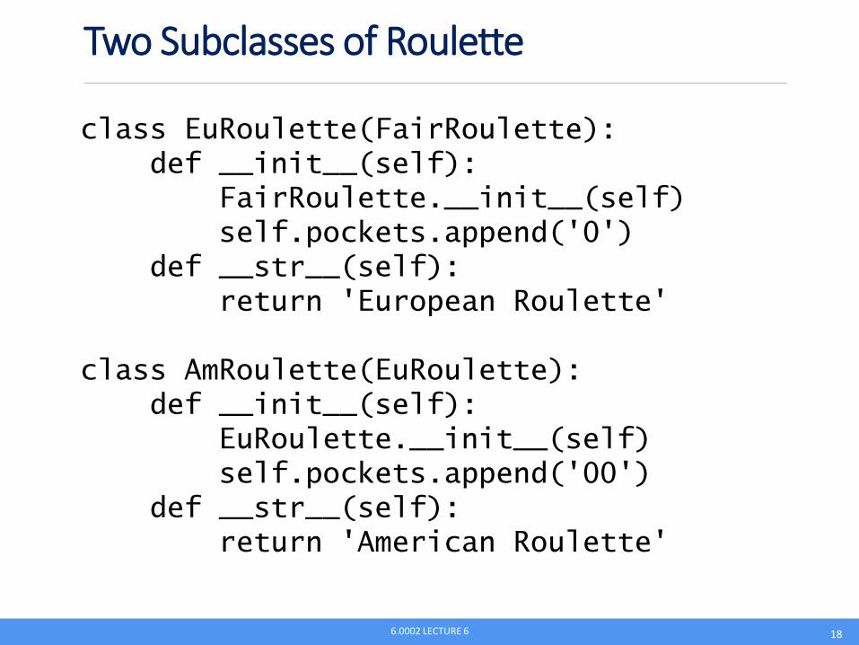
Two Subclasses of Roulette

class EuRoulette(FairRoulette): def __init__(self):

FairRoulette.__init__(self) self.pockets.append('0')

def __str__(self): return 'European Roulette'

class AmRoulette(EuRoulette): def __init__(self):

EuRoulette.__init__(self) self.pockets.append('00')

def __str__(self): return 'American Roulette'

6.0002 LECTURE 6 18

Comparing the Games Simulate 20 trials of 1000 spins each Exp. return for Fair Roulette = 6.56% Exp. return for European Roulette = -2.26% Exp. return for American Roulette = -8.92%

Simulate 20 trials of 10000 spins each Exp. return for Fair Roulette = -1.234% Exp. return for European Roulette = -4.168% Exp. return for American Roulette = -5.752%

Simulate 20 trials of 100000 spins each Exp. return for Fair Roulette = 0.8144% Exp. return for European Roulette = -2.6506% Exp. return for American Roulette = -5.113%

Simulate 20 trials of 1000000 spins each Exp. return for Fair Roulette = -0.0723% Exp. return for European Roulette = -2.7329%

6.0002 LECTURE 6

Exp. return for American Roulette = -5.212%

19

Sampling Space of Possible Outcomes

Never possible to guarantee perfect accuracy through sampling

Not to say that an estimate is not precisely correct

Key question: ◦ How many samples do we need to look at before we can

have justified confidence on our answer?

Depends upon variability in underlying distribution

6.0002 LECTURE 6 20

Standard deviation simply the square root of the variance

Outliers can have a big effect

Standard deviation should always be considered relative to mean

Quantifying Variation in Data

6.0002 LECTURE 6

 

1(X) (x )2

X xX

21

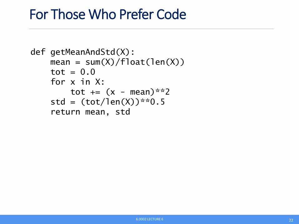
For Those Who Prefer Code

def getMeanAndStd(X): mean = sum(X)/float(len(X)) tot = 0.0 for x in X:

tot += (x - mean)**2 std = (tot/len(X))**0.5 return mean, std

6.0002 LECTURE 6 22

Confidence Levels and Intervals

Instead of estimating an unknown parameter by a single value (e.g., the mean of a set of trials), a confidence interval provides a range that is likely to contain the unknown value and a confidence that the unknown value lays within that range

ϮϴϪή ή ΟήϭϠ Β Πϼή ϭͼϼ ϭή ϭ EήΒ roulette is -3.3%. The margin of error is +/- 3.5% with a 95% level of confidenceϨϯ What does this mean?

If I were to conduct an infinite number of trials of 10k bets each, ◦ My expected average return would be -3.3% ◦ My return would be between roughly -6.8% and +0.2% 95% of

the time

6.0002 LECTURE 6 23

Empirical Rule

Under some assumptions discussed later ◦ ~68% of data within one standard deviation of mean ◦ ~95% of data within 1.96 standard deviations of mean ◦ ~99.7% of data within 3 standard deviations of mean

6.0002 LECTURE 6 24

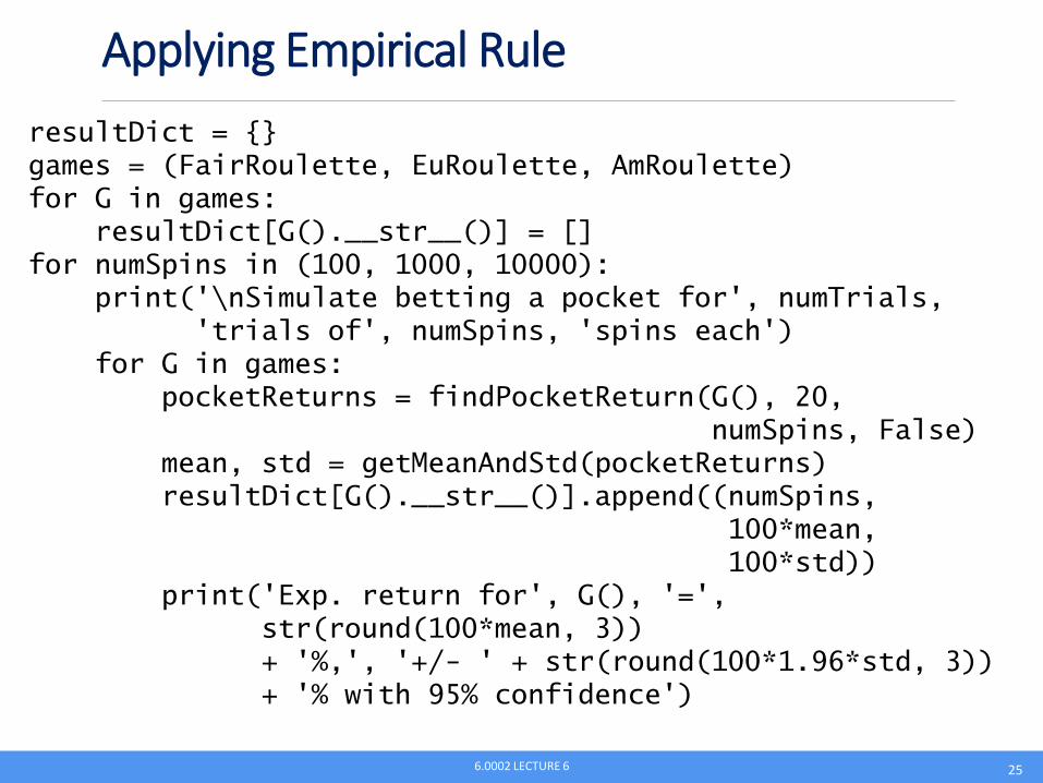
Applying Empirical Rule resultDict = {} games = (FairRoulette, EuRoulette, AmRoulette) for G in games:

resultDict[G().__str__()] = [] for numSpins in (100, 1000, 10000):

print('\nSimulate betting a pocket for', numTrials, 'trials of', numSpins, 'spins each')

for G in games: pocketReturns = findPocketReturn(G(), 20,

numSpins, False) mean, std = getMeanAndStd(pocketReturns) resultDict[G().__str__()].append((numSpins,

100*mean, 100*std))

print('Exp. return for', G(), '=', str(round(100*mean, 3)) + '%,', '+/- ' + str(round(100*1.96*std, 3)) + '% with 95% confidence')

6.0002 LECTURE 6 25

Results Simulate betting a pocket for 20 trials of 1000 spins each Exp. return for Fair Roulette = 3.68%, +/- 27.189% with 95% confidence Exp. return for European Roulette = -5.5%, +/- 35.042% with 95% confidence Exp. return for American Roulette = -4.24%, +/- 26.494% with 95% confidence

Simulate betting a pocket for 20 trials of 100000 spins each Exp. return for Fair Roulette = 0.125%, +/- 3.999% with 95% confidence Exp. return for European Roulette = -3.313%, +/- 3.515% with 95% confidence Exp. return for American Roulette = -5.594%, +/- 4.287% with 95% confidence

Simulate betting a pocket for 20 trials of 1000000 spins each Exp. return for Fair Roulette = 0.012%, +/- 0.846% with 95% confidence Exp. return for European Roulette = -2.679%, +/- 0.948% with 95% confidence Exp. return for American Roulette = -5.176%, +/- 1.214% with 95% confidence

6.0002 LECTURE 6 26

Assumptions Underlying Empirical Rule

The mean estimation error is zero

The distribution of the errors in the estimates is normal

6.0002 LECTURE 6 27

Defining Distributions

Use a probability distribution

Captures notion of relative frequency with which a random variable takes on certain values ◦ Discrete random variables drawn from finite set of values ◦ Continuous random variables drawn from reals between

two numbers (i.e., infinite set of values)

For discrete variable, simply list the probability of each value, must add up to 1

Cϭ ΠΒή ϭΠϼϭή ϥ ΠΒϫ ήήΒή ΟΒΟϭϿϭ for each of an infinite set of values

6.0002 LECTURE 6 28

PDF’s

Distributions defined by probability density functions (PDFs)

Probability of a random variable lying between two values

Defines a curve where the values on the x-axis lie between minimum and maximum value of the variable

Area under curve between two points, is probability of example falling within that range

6.0002 LECTURE 6 29

Normal Distributions

6.0002 LECTURE 6

e 1n!n0

~68% of data within one standard deviation of mean

~95% of data within 1.96 standard deviations of mean

~99.7% of data within 3 standard deviations of mean

30

MIT OpenCourseWarehttps://ocw.mit.edu

6.0002 Introduction to Computational Thinking and Data ScienceFall 2016

For information about citing these materials or our Terms of Use, visit: https://ocw.mit.edu/terms.