Lecture 6: Edge Detection - University of...

ME5286 – Lecture 6

Lecture 6: Edge Detection

Saad J [email protected]

#1


Review From Last Lecture

• Options for Image Representation– Introduced the concept of different

representation or transformation• Fourier Transform

– Opportunity of manipulate, process and analyze the image in a frequency domain

• Frequency Domain Filtering– Can be more efficient in certain cases

#2


Frequency Domain Methods

Spatial DomainFrequency Domain


Major filter categories

• Typically, filters are classified by examining their properties in the frequency domain:

(1) Low-pass (2) High-pass (3) Band-pass (4) Band-stop


Example

Original signal

Low-pass filtered

High-pass filtered

Band-pass filtered

Band-stop filtered


Low-pass filters (i.e., smoothing filters)

• Preserve low frequencies - useful for noise suppression

frequency domain time domain

Example:


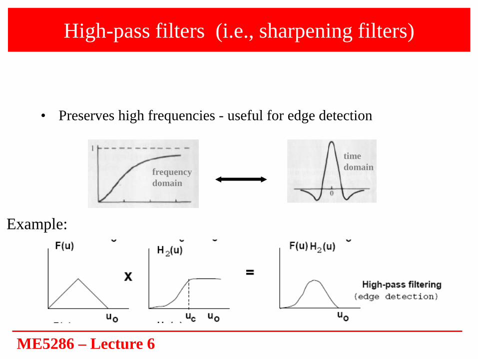
High-pass filters (i.e., sharpening filters)

• Preserves high frequencies - useful for edge detection

frequency domain

timedomain

Example:


Band-pass filters

• Preserves frequencies within a certain band

frequency domain

timedomain

Example:


Band-stop filters

• How do they look like?Band-pass Band-stop


Frequency Domain Methods

Case 1: H(u,v) is specified inthe frequency domain.

Case 2: h(x,y) is specified inthe spatial domain.


Frequency domain filtering: steps

F(u,v) = R(u,v) + jI(u,v)


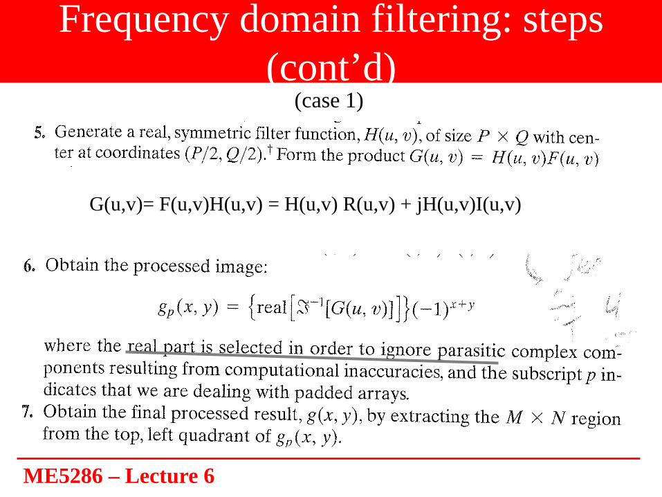
Frequency domain filtering: steps (cont’d)

G(u,v)= F(u,v)H(u,v) = H(u,v) R(u,v) + jH(u,v)I(u,v)

(case 1)


Example

f(x,y) fp(x,y) fp(x,y)(-1)x+y

F(u,v)H(u,v) - centered G(u,v)=F(u,v)H(u,v)

g(x,y)gp(x,y)


h(x,y) specified in spatial domain:how to generate H(u,v) from h(x,y)?

• If h(x,y) is given in the spatial domain (case 2), we can generate H(u,v) as follows:

1.Form hp(x,y) by padding with zeroes.

2. Multiply by (-1)x+y to center its spectrum.

3. Compute its DFT to obtain H(u,v)


Edge Detection

• Definition of an Edge• Edge Modeling and Edge Descriptors• Edge Detection Methods

– First and Second Derivative Approximations

#15


Image Segmentation• Image segmentation methods will look for objects

that either have some measure of homogeneitywithin themselves, or have some measure of contrast with the objects on their border

• The homogeneity and contrast measures can include features such as gray level, color, and texture

#16


Edge Detection: First Step to Image Segmentation

• The goal of image segmentation is to find regions that represent objects or meaningful parts of objects

• Division of the image into regions corresponding to objects of interest is necessary for scene interpretation and understanding

• Identification of real objects, pseudo-objects, shadows, or actually finding anything of interest within the image, requires some form of segmentation

#17


Image Edges

Image Features that are Local, meaningful, detectable parts of the image.

#18


Edge Detection Objectives

• Edge detection operators are used as a first step in the line (or curve) detection process.

• Edge detection is also used to find complex object boundaries by marking potential edge points corresponding to places in an image where rapid changes in brightness occur

#19


Edge Detection Objectives

• After the edge points have been marked, they can be merged to form a line/curves or object outlines

• A curve is a continuous collection of edge points along a certain direction

• Different methods can use the edge information to construct meaningful regions for image analysis

#20


Edges & Lines Relationship

Edge

Line

Edge

The line shown here is vertical and the edge direction is horizontal. In this case the transition from black to white occurs along a row, this is the edge direction, but the line is vertical along a column.

Edges and lines are perpendicular

#21


Definition of Edges

• Edges are significant local changes of intensity in an image.


Why is Edge Detection Useful?

• Important features can be extracted from the edges of an image (e.g., corners, lines, curves).

• These features are used by higher-level computer vision algorithms (e.g., recognition).


Goals of Edge Detection• Goal of Edge Detection

– Produce a line drawing of a scene from an image of that scene.

– Important features can be extracted from the edges of an image (e.g., corners, lines, curves).

– These features are used by higher-level computer vision algorithms (e.g., segmentation, recognition).

#24


Challenges: Effect of Illumination


Goals of an Edge Detector

• Goal to construct edge detection operators that extracts– the orientation information (information about the

direction of the edge) and – the strength of the edge. Some methods can return information about the existence of an edge at each point for faster processing

#26


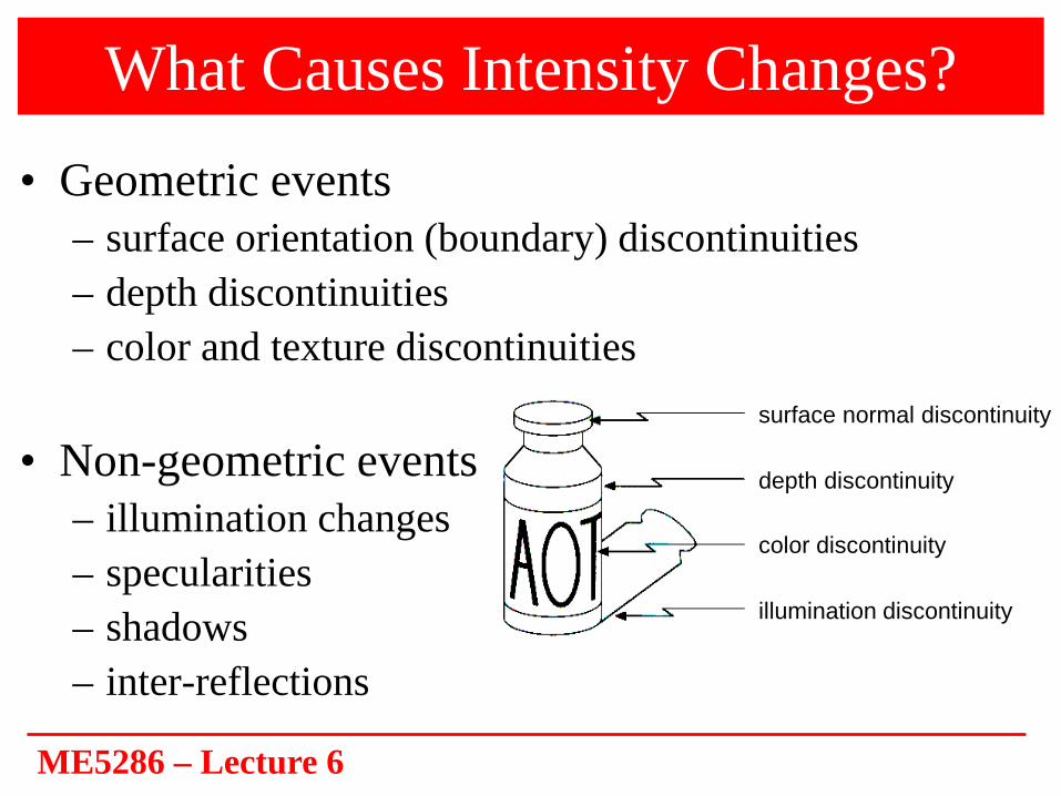
What Causes Intensity Changes?• Geometric events

– surface orientation (boundary) discontinuities– depth discontinuities– color and texture discontinuities

• Non-geometric events– illumination changes– specularities– shadows– inter-reflections

depth discontinuity

color discontinuity

illumination discontinuity

surface normal discontinuity


What Causes Intensity Changes?

Depth discontinuity: object boundary

Change in surface orientation: shape

Cast shadows

Reflectance change: appearance information, texture


Good Examples: Edge Detection

• Minimal Noise in the Image

#29


Example: Edge Detection

• Different scales of edges ( Hair , Face, … )#30


• Challenge to extract meaningful edges not corrupted by Noise

Edge DetectionExample: Edge Detection


Modeling Intensity Changes

• Step edge: the image intensity abruptly changes from one value on one side of the discontinuity to a different value on the opposite side.


Modeling Intensity Changes (cont’d)

• Ridge edge: the image intensity abruptly changes value but then returns to the starting value within some short distance (i.e., usually generated by lines).



• Roof edge: a ridge edge where the intensity change is not instantaneous but occur over a finite distance (i.e., usually generated by the intersection of two surfaces).



• Ramp edge: a step edge where the intensity change is not instantaneous but occur over a finite distance.


Summary: Edge Definition• Edge is a boundary between two regions with relatively distinct gray level

properties. • Edges are pixels where the brightness function changes abruptly. • Edge detectors are a collection of very important local image pre-

processing methods used to locate (sharp) changes in the intensity function.

#36


Edge Descriptors• Edge descriptors

– Edge normal: unit vector in the direction of maximum intensity change.

– Edge direction: unit vector to perpendicular to the edge normal.

– Edge position or center: the image position at which the edge is located.

– Edge strength: related to the local image contrast along the normal.

#37


What are the steps for Edge Detection

• Main Steps in Edge Detection(1) Smoothing: suppress as much noise as possible, without destroying true edges.( we talked about this step before )

(2) Enhancement: apply differentiation to enhance the quality of edges (i.e., sharpening).


Main Steps in Edge Detection (cont’d)

(3) Thresholding: determine which edge pixels should be discarded as noise and which should be retained (i.e., threshold edge magnitude).

(4) Localization: determine the exact edge location.

sub-pixel resolution might be required for some applications to estimate the location of an edge to better than the spacing between pixels.


Edge Detection using Derivatives• Edge detection using derivatives

– Calculus describes changes of continuous functions using derivatives.

– An image is a 2D function, so operators describing edges are expressed using partial derivatives.

– Points which lie on an edge can be detected by either:• detecting local maxima or minima of the first derivative• detecting the zero-crossing of the second derivative

#40


1st order derivatives Interpretation


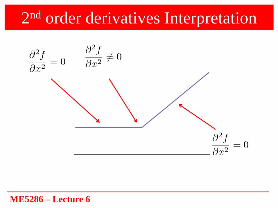
2nd order derivatives Interpretation


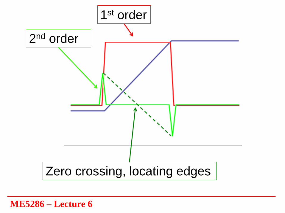
1st order

2nd order

Zero crossing, locating edges


Comparison of Derivatives

• Looking at “nonzero-ness”– 1st order derivative gives thick edges– 2nd order derivative gives double edge

• 2nd order derivatives enhance fine detail much better.

44


1st order

2nd order

Zero crossing, locating edges


Edge Detection Using Derivatives

• Often, points that lie on an edge are detected by:

(1) Detecting the local maxima or minima of the first derivative.

(2) Detecting the zero-crossingsof the second derivative. 2nd derivative

1st derivative


Image Derivatives

• How can we differentiate a digital image?

– Option 1: reconstruct a continuous image, f(x,y), then compute the derivative.

– Option 2: take discrete derivative (i.e., finite differences)

Pick Option 2 for Digital Processing


Edge Detection using DerivativesFor 2D function, f(x,y), the partial derivative is:

For discrete data, we can approximate using finite differences:

To implement above as convolution, what would be the associated filter? [-1 1] or [1 -1] ?

εε

ε

),(),(lim),(0

yxfyxfx

yxf −+=

∂∂

→

1),(),1(),( yxfyxf

xyxf −+

≈∂

∂


Edge Detection Using First Derivative • Computing the 1st derivative – cont.

)1()1()( −−+=′ xfxfxf

)()1()( xfxfxf −+=′

)1()()( −−≈′ xfxfxf Backward difference

Forward difference

Central difference

#49


Edge Detection Using First Derivative

• Cartesian vs pixel-coordinates: - j corresponds to x direction

- i to -y direction



sensitive to vertical edges!

sensitive to horizontal edges!



ramp edge

roof edge

(upward) step edge

(downward) step edge

(centered at x)

1D functions(not centered at x)


Edge Detection Using First Derivative • Computing the 1st derivative – cont.

– Examples using the edge models and the mask [ -1 0 1] (centered about x):

#53



Which shows changes with respect to x?

-1 1

1 -1or

?-1 1

xyxf

∂∂ ),(

yyxf

∂∂ ),(


• We can implement and using the following masks:

(x+1/2,y)

(x,y+1/2) **

good approximationat (x+1/2,y)

good approximationat (x,y+1/2)



• A different approximation of the gradient:

• and can be implemented using the following masks:

*

(x+1/2,y+1/2)good approximation



Approximation of First Derivative ( Gradient )

• Consider the arrangement of pixels about the pixel (i, j):

• The partial derivatives can be computed by:

• The constant c implies the emphasis given to pixels closer to the center of the mask.

3 x 3 neighborhood:


Prewitt Operator

• Setting c = 1, we get the Prewitt operator:


Sobel Operator

• Setting c = 2, we get the Sobel operator:


Edge Detection Steps Using Gradient

(i.e., sqrt is costly!)


Example (using Prewitt operator)

Note: in this example, thedivisions by 2 and 3 in the computation of fx and fyare done for normalization purposes only


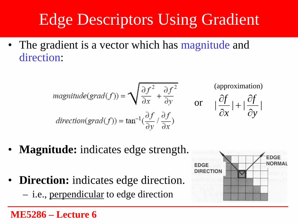
• The gradient is a vector which has magnitude and direction:

• Magnitude: indicates edge strength.

• Direction: indicates edge direction.– i.e., perpendicular to edge direction

| | | |f fx y∂ ∂

+∂ ∂

or

(approximation)

Edge Descriptors Using Gradient


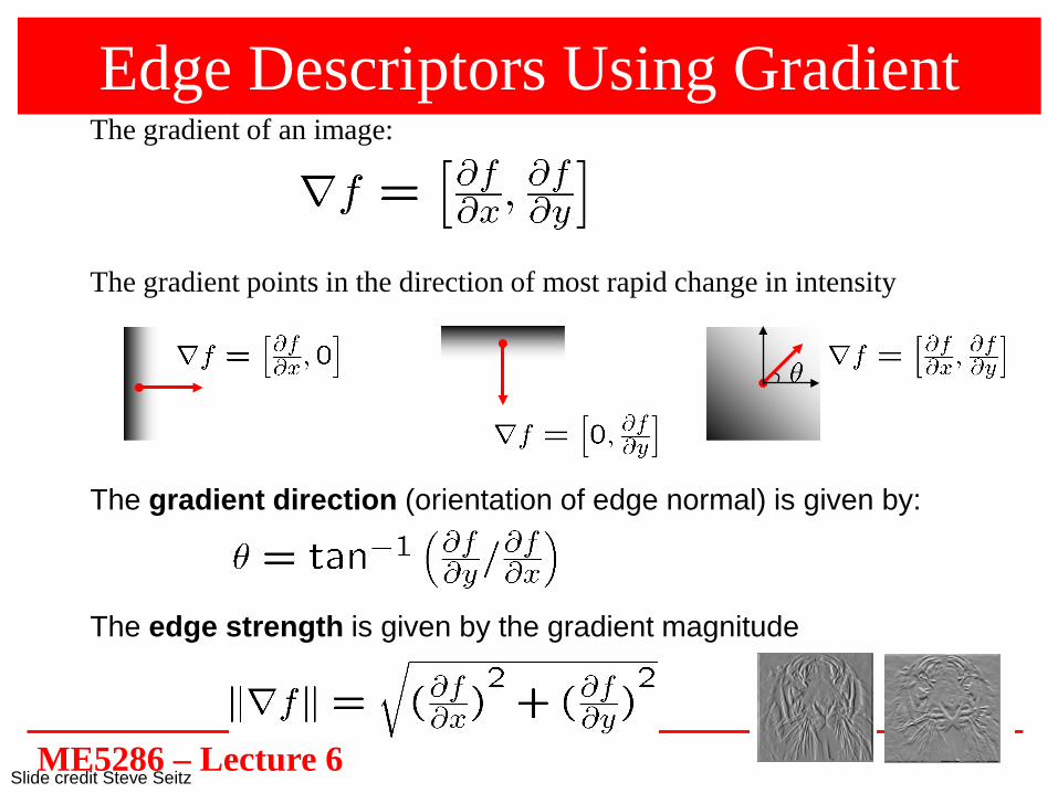
Edge Descriptors Using GradientThe gradient of an image:

The gradient points in the direction of most rapid change in intensity

The gradient direction (orientation of edge normal) is given by:

The edge strength is given by the gradient magnitude

Slide credit Steve Seitz


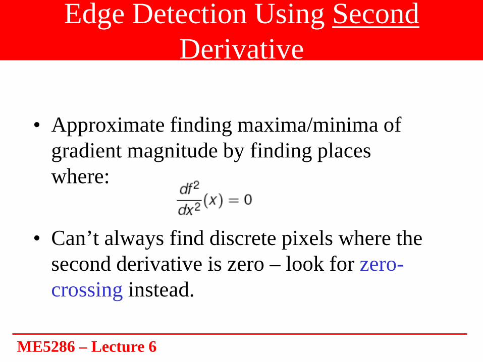
Edge Detection Using SecondDerivative

• Approximate finding maxima/minima of gradient magnitude by finding places where:

• Can’t always find discrete pixels where the second derivative is zero – look for zero-crossing instead.


Edge Detection Using Second Derivative• Computing the 2nd derivative:

– This approximation is centered about x + 1– By replacing x + 1 by x we obtain:

#65


Image Derivatives

• 1st order

• 2nd order


Edge Detection Using Second Derivative (cont’d)



• Computing the 2nd derivative – cont.– Examples using the edge models:

#68



(upward) step edge

(downward) step edge

ramp edge

roof edge



• Four cases of zero-crossings:

{+,-}, {+,0,-},{-,+}, {-,0,+}

• Slope of zero-crossing {a, -b} is: |a+b|.

• To detect “strong” zero-crossing, threshold the slope.


Noise Effect on Derivates

Where is the edge??


Solution: smooth first

Where is the edge? Look for peaks in


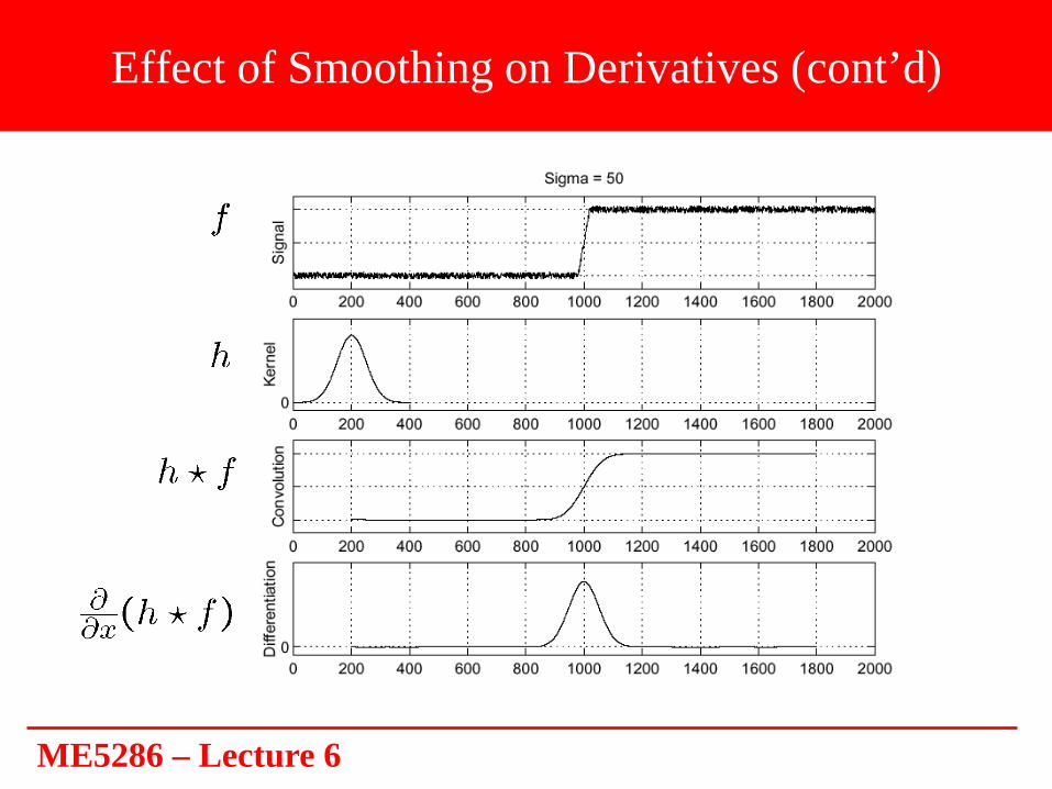
Effect of Smoothing on Derivatives (cont’d)


Combine Smoothing with Differentiation

(i.e., saves one operation)


Laplacian of GaussianConsider

Laplacian of Gaussianoperator

Where is the edge? Zero-crossings of bottom graphSlide credit: Steve Seitz


2D edge detection filters

• is the Laplacian operator:

Laplacian of Gaussian

Gaussian derivative of Gaussian

Slide credit: Steve Seitz


[ ]11 −⊗[ ]0.0030 0.0133 0.0219 0.0133 0.00300.0133 0.0596 0.0983 0.0596 0.01330.0219 0.0983 0.1621 0.0983 0.02190.0133 0.0596 0.0983 0.0596 0.01330.0030 0.0133 0.0219 0.0133 0.0030

)()( hgIhgI ⊗⊗=⊗⊗

Derivative of Gaussian filters


Derivative of Gaussian filters

x-direction y-direction

Source: L. Lazebnik


Smoothing with a GaussianRecall: parameter σ is the “scale” / “width” / “spread” of the Gaussian kernel, and controls the amount of smoothing.

…


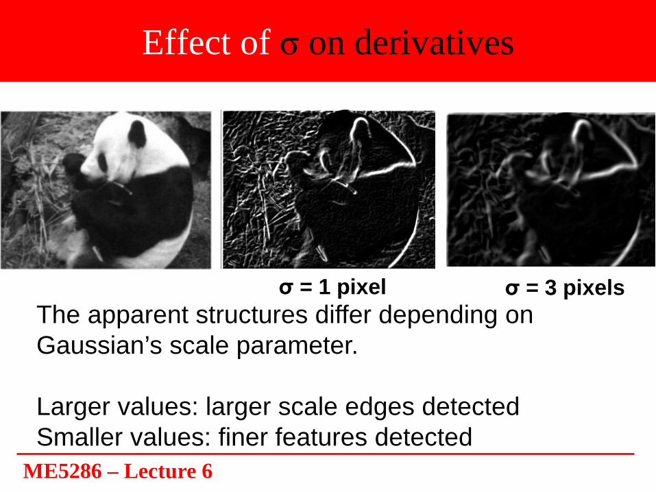
Effect of σ on derivatives

The apparent structures differ depending on Gaussian’s scale parameter.

Larger values: larger scale edges detectedSmaller values: finer features detected

σ = 1 pixel σ = 3 pixels


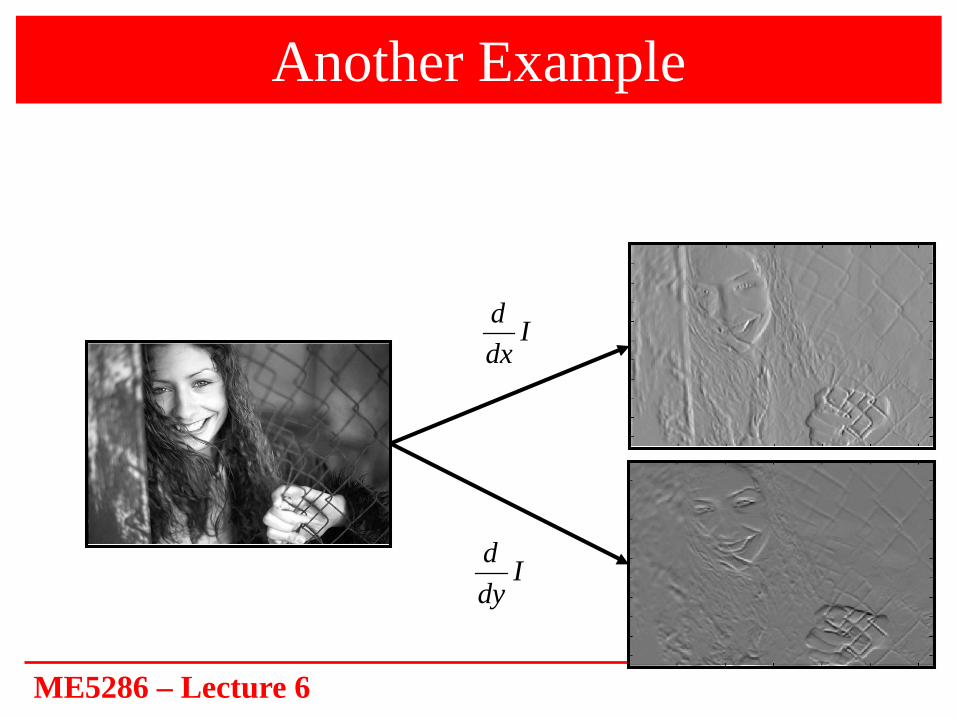
Another Example

Idxd

Idyd


Another Example (cont’d)

22d dI Idx dy

∇ = +

100Threshold∇ ≥ =


Isotropic property of gradient magnitude

• The magnitude of the gradient detects edges in all directions.

22d dI Idx dy

∇ = +

Idxd I

dyd


Second Derivative in 2D: Laplacian


Variations of Laplacian


Laplacian - Example

detect zero-crossings


Properties of Laplacian

• It is an isotropic operator. • It is cheaper to implement than the gradient

(i.e., one mask only). • It does not provide information about edge

direction.• It is more sensitive to noise (i.e.,

differentiates twice).


Laplacian of Gaussian (LoG)(Marr-Hildreth operator)

• To reduce the noise effect, the image is first smoothed. • When the filter chosen is a Gaussian, we call it the LoG

edge detector.

• It can be shown that:

σ controls smoothing

2σ2

(inverted LoG)


Laplacian of Gaussian (LoG) -Example

filtering zero-crossings

(inverted LoG)(inverted LoG)


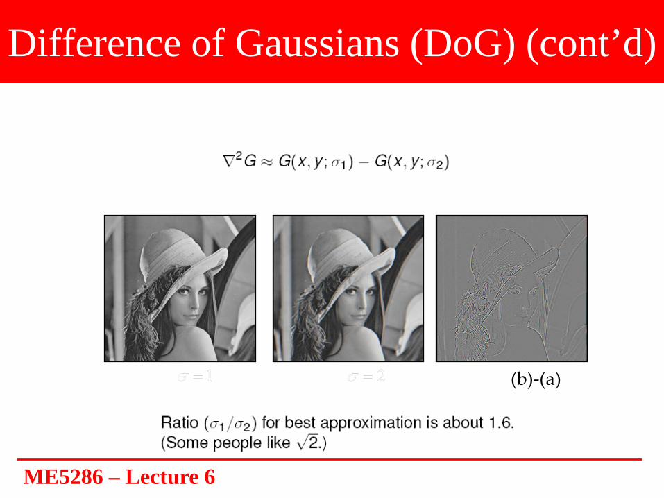
Difference of Gaussians (DoG)• The Laplacian of Gaussian can be approximated by the

difference between two Gaussian functions:

approximationactual LoG


Difference of Gaussians (DoG) (cont’d)

(a) (b) (b)-(a)


Gradient vs LoG• Gradient works well when the image contains sharp

intensity transitions and low noise.• Zero-crossings of LOG offer better localization, especially

when the edges are not very sharp.step edge

ramp edge


Gradient vs LoG (cont’d)

LoG behaves poorly at corners


Criteria for Optimal Edge Detection

• (1) Good detection– Minimize the probability of false positives (i.e., spurious edges).– Minimize the probability of false negatives (i.e., missing real

edges).

• (2) Good localization– Detected edges must be as close as possible to the true edges.

• (3) Single response– Minimize the number of local maxima around the true edge.


Practical Issues

• Noise suppression-localization tradeoff.– Smoothing depends on mask size (e.g., depends

on σ for Gaussian filters).– Larger mask sizes reduce noise, but worsen

localization (i.e., add uncertainty to the location of the edge) and vice versa.

larger masksmaller mask


Practical Issues (cont’d)• Choice of threshold.

gradient magnitude

low threshold high threshold


Standard thresholding• Standard thresholding:

- Can only select “strong” edges.- Does not guarantee “continuity”.

gradient magnitude low threshold high threshold


Hysteresis thresholding

• Hysteresis thresholding uses two thresholds:

• For “maybe” edges, decide on the edge if neighboringpixel is a strong edge.

- low threshold tl- high threshold th (usually, th = 2tl)

tltl

th

th


Directional Derivative

• The partial derivatives of f(x,y) will give the slope ∂f/∂x in the positive x direction and the slope ∂f /∂y in the positive y direction.

• We can generalize the partial derivatives to calculate the slope in any direction (i.e., directional derivative).

f∇


Directional Derivative (cont’d)

• Directional derivative computes intensity changes in a specified direction.

Compute derivative in direction u



+ =

Directional derivative is a

linear combination of

partial derivatives.

(From vector calculus)



+ =cosθ sinθ

cos , sin yx uuu u

θ θ= = cos , sinx yu uθ θ= =||u||=1


Edge Detection Review

• Edge detection operators are based on the idea that edge information in an image is found by looking at the relationship a pixel has with its neighbors

• If a pixel's gray level value is similar to those around it, there is probably not an edge at that point

#104


Edge Detection Review

• Edge detection operators are often implemented with convolution masks and most are based on discrete approximations to differential operators

• Differential operations measure the rate of change in a function, in this case, the image brightness function

#105


Edge Detection Review• Preprocessing of image is required to eliminate or

at least minimize noise effects• There is tradeoff between sensitivity and accuracy

in edge detection • The parameters that we can set so that edge

detector is sensitive include the size of the edge detection mask and the value of the gray level threshold

• A larger mask or a higher gray level threshold will tend to reduce noise effects, but may result in a loss of valid edge points

#106

Lecture 6: Edge Detection - University of...

Documents

Transcript of Lecture 6: Edge Detection - University of...