Lecture 5:Mean-Reversion

Marco Avellaneda

G63.2936.001

Spring Semester 2009

Stationarity/ Non Stationarity

Definition: a stochastic process is stationary if

( )( ){ } ( ){ }AXXXAXXX

Attm

hththtttt

nm

mm∈=∈

∈∀∀∀

+++ ,...,,.Pr,...,,.Pr

,,..., ,

2121

1 R

A stationary process is a process that is ``statistically invariant under translations’’

Examples: the Ornstein-Uhlembeck process is stationary, Brownian motionis not.

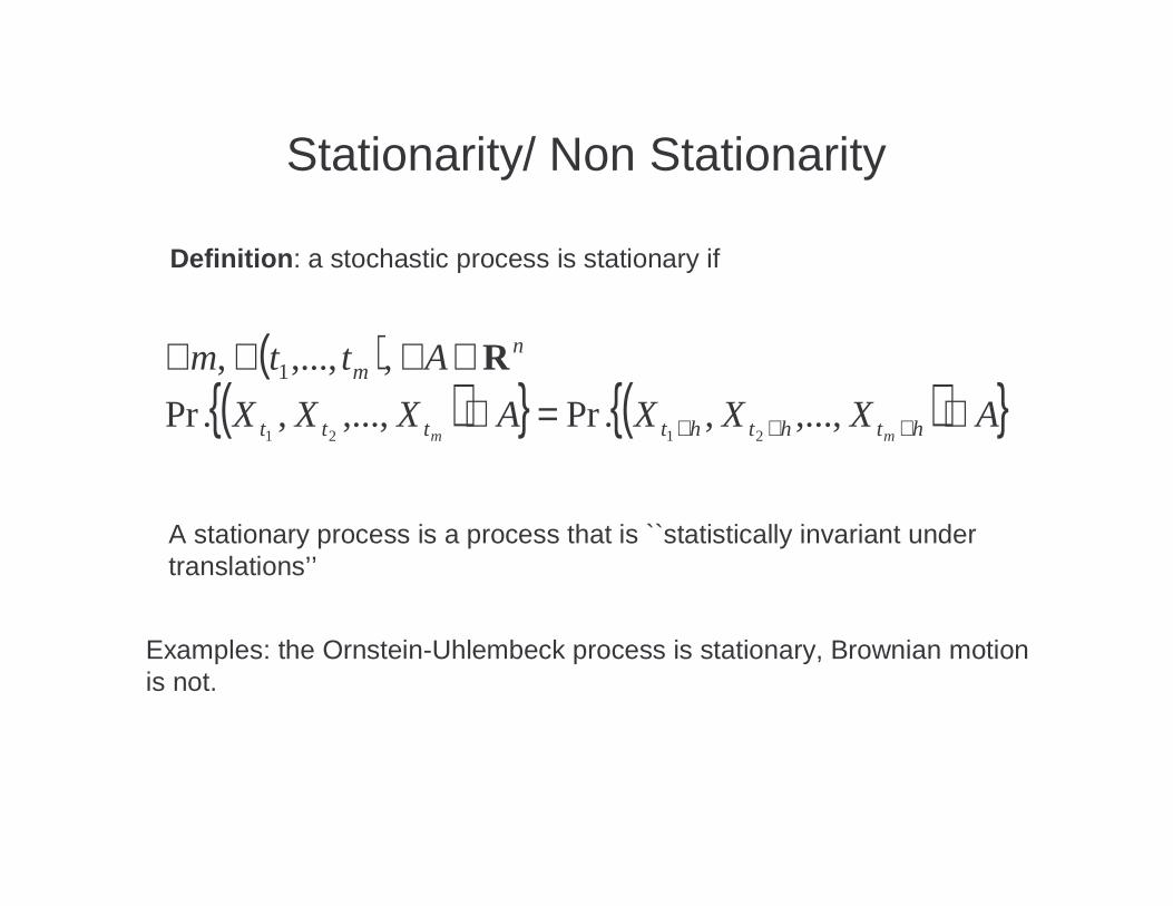
The Ornstein-Uhlenbeck process

( )

( ) ( )( ) ( )

( ) ( ) ( ) noise hiteGaussian w ,

1

=+=

+−+=

+−=

∫

∫

∞−

−−

−−−−−−

sdssemX

dWemeXeX

dWdtXmdX

tst

t

u

t

s

utsts

stt

ttt

ηησ

σ

σκ

κ

κκκ

Exponentially-weighted moving average of uncorrelated Gaussianrandom variables.

Statistics of the OU process

( ) ( ) ( ) ( )( ) ( ) ( )

( ) ( )

( )

( )khtht

kh

t stkkh

t shtkstk

t ht shtkstk

t ht shtkstkhtt

ek

XX

k

e

dsee

dsee

dsdsssee

dssedsseXX

−+

−

∞−

−−−

∞−

−+−−−

∞−

+

∞−

−+−−−

∞−

+

∞−

−+−−−+

−=−

=

=

=

−=

⋅=

∫

∫

∫ ∫

∫ ∫

1

2

''

''

22

2

22

2

'2

'2

σ

σ

σ

σ

δσ

ηησ

Structure Function

Random Walk, Fractional BM

( )( )

>

=

<<

≈

+=

>−+

=

==−

==

−

+

∞

−+

∞−

++

∫

∫

1

1 )ln(

12/1

)1(

2/1 1

motionBrownian ,

2

2

12

2

112

2

22

ph

ph

h

ph

XX

uu

du

hXX

pst

dssX

tXXhXX

WWX

p

p

htt

h

ppphtt

t

pt

thttht

ttt

σ

σ

σ

σ

ησ

σ

σ Brownian motion (non-stationary)Structure fn grows linearly

Geometric Brownian motion

Correlations decay like power-laws(large h)

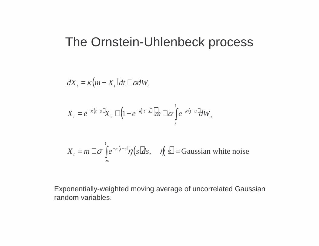
Autoregressive Models

( )

10

0

0

1

1

11101

21

1

...

0 ,

...

0 ,

01...

...01

...

,...

1,0~ ,...

,...,...,,

+

+−

++−+

++=

=

=

=

=

++++=

+ n

m

mn

n

inmnmnn

n

nn

n

aaa

X

X

NXaXaaX

XXX

ν

σ

νσν

ΣAYAY

ΣAAY

AR-n model corresponds to a vector AR-1 model

Structure function: SPY Jan 1996-Jan 2009

Use log prices as time series. Structure function with lags 1 day to 2 yrs

0

0.01

0.02

0.03

0.04

0.05

0.06

0.07

0.08

0.09

0.1

1 27 53 79 105 131 157 183 209 235 261 287 313 339 365 391 417 443 469 495

SPY is highly non stationary, as shown in the chart.Look for mean-reversion in relative value, i.e. in terms of two or more assets.

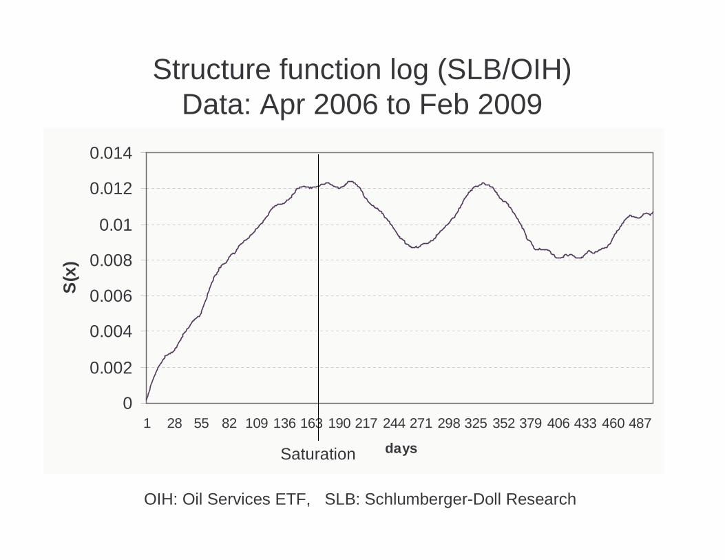
Structure function log (SLB/OIH)Data: Apr 2006 to Feb 2009

0

0.002

0.004

0.006

0.008

0.01

0.012

0.014

1 28 55 82 109 136 163 190 217 244 271 298 325 352 379 406 433 460 487

days

S(x

)

Saturation

OIH: Oil Services ETF, SLB: Schlumberger-Doll Research

Structure Function: long-shortequal dollar weighted SLB-OIH

0

0.005

0.01

0.015

0.02

0.025

1 24 47 70 93 116 139 162 185 208 231 254 277 300 323 346 369 392 415 438 461 484

days

S(x

)

( ) nnnn PXRRPP ln ,1 oihslb1 =−+×=+

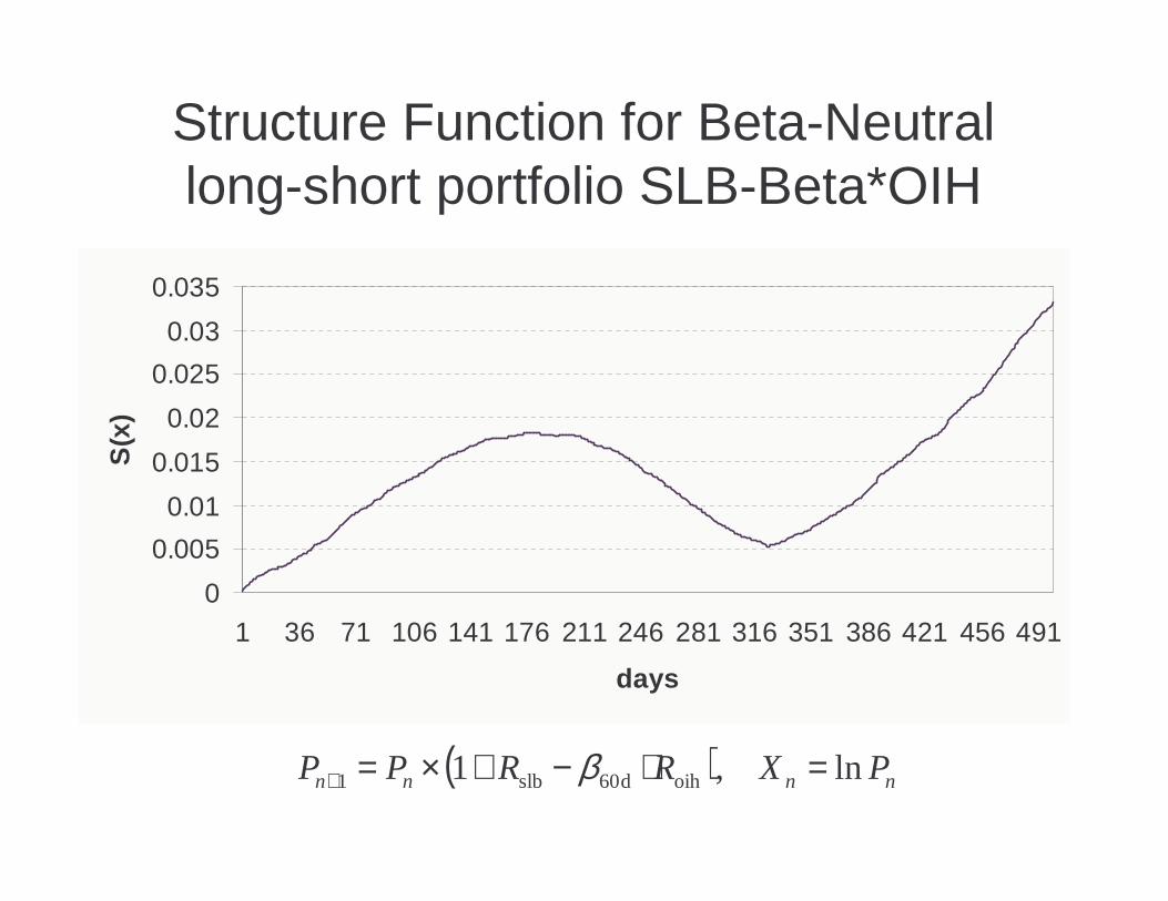
Structure Function for Beta-Neutrallong-short portfolio SLB-Beta*OIH

0

0.005

0.01

0.015

0.02

0.025

0.03

0.035

1 36 71 106 141 176 211 246 281 316 351 386 421 456 491

days

S(x

)

( ) nnnn PXRRPP ln ,1 oihd60slb1 =⋅−+×=+ β

Structure Function log (GENZ/IBB)

0

0.01

0.02

0.03

0.04

0.05

0.06

0.07

1 35 69 103 137 171 205 239 273 307 341 375 409 443 477

days

S(x

)

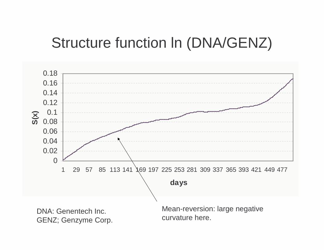
Structure function ln (DNA/GENZ)

00.020.040.060.080.1

0.120.140.160.18

1 29 57 85 113 141 169 197 225 253 281 309 337 365 393 421 449 477

days

S(x

)

DNA: Genentech Inc.GENZ; Genzyme Corp.

Mean-reversion: large negativecurvature here.

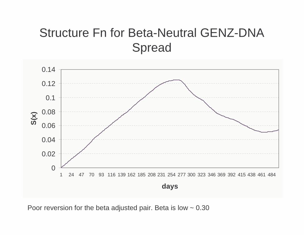
Structure Fn for Beta-Neutral GENZ-DNA Spread

0

0.02

0.04

0.06

0.08

0.1

0.12

0.14

1 24 47 70 93 116 139 162 185 208 231 254 277 300 323 346 369 392 415 438 461 484

days

S(x

)

Poor reversion for the beta adjusted pair. Beta is low ~ 0.30

Systematic Approach for looking for MR in Equities

Look for stock returns devoid of explanatory factors, and analyze thecorresponding residuals as stochastic processes.

( )( )

( )( ) ( )tdXtP

tdP

tS

tdS

XX

FR

k

km

kk

t

sst

tkt

m

kkt

+=

+=

+=

∑

∑

∑

=

=

=

1

10

1

β

ε

εβ Econometric factor model

View residuals as increments of aprocess that will be estimated

Continuous-time model for evolutionof stock price

Interpretation of the model

The factors are either

A. eigenportfolios corresponding to significant eigenvaluesof the market

B. industry ETF, or portfolios of ETFs

Questions of interest:

Can residuals be fitted to (increments of) OU processes orother MR processes?

If so, what is the typical correlation time-scale?

Estimation of Ornstein-Uhlenbeck models

( ) ( )

{ }

−++=

+−+=

∆−

++

∆+−−∆−∆−

∆+ ∫

k

eNbaXX

dWeemXeX

tk

nnnn

tt

t

sstktk

ttk

tt

2

1,0 i.i.d.

1

22

11 σνν

σ

( ) ( )( )( ) ( )( )

( )

∆−−−=

−=

∆=

==

+

−−−−

−−−−

ata

baXX

a

bm

atk

XXXXb

XXXXa

nn

nlnnln

nlnnln

1ln

12

1

STDEV ,

1 ,

1ln

1

,...,;,...,INTERCEPT

,,...,;,...,SLOPE

2

1

11

11

σ

Portfolio Strategy

portfolio of exposuredollar net :

factor along exposure beta-dollarnet :

costs) ransaction(neglect t

prices adjusted-dividend ,.....,,

short)or (long stocksdifferent in invested $ ,....,,

1

1

11 11

111

11

21

21

−

+=

−

+=

−=Π

∑

∑

∑∑ ∑∑

∑∑∑

∑∑

=

=

== ==

===

==

N

ii

N

iiki

N

ii

m

k k

kN

iikii

N

ii

N

ii

m

ki

k

kik

N

ii

N

ii

i

iN

ii

N

N

Q

kQ

rdtQP

dPQdXQ

rdtQdXP

dPQ

rdtQS

dSQd

SSS

QQQ

β

β

β

Market-Neutral Portfolio

( ) { }

( )( )

( )( )

( ) ( )( )

( ) dtQdVar

dtrXmkQdE

dWQdtrXmkQ

rdtQdWdtXmkQ

rdtQdXQd

dWdWdtXmkdX

i

N

i

i

ii

N

ii

ii

N

iiii

N

ii

N

iiiiii

N

ii

N

iii

N

ii

N

iiiiiii

2

1

2

1

11

11

11

1

|

|

eduncorrelat Assume

σ

σ

σ

σ

∑

∑

∑∑

∑∑

∑∑

=

=

==

==

==

=

=Π

−−=Π

∴

+−−=

−+−=

−=Π

+−=

X

X

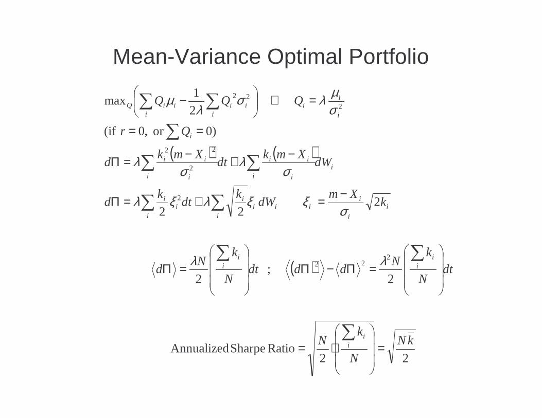
Mean-Variance Optimal Portfolio

( ) ( )

( )

22Ratio Sharpe Annualized

2 ;

2

2 22

)0or ,0 if(

2

1max

222

2

2

22

222

kN

N

kN

dtN

kN

dddtN

kN

d

kXm

dWk

dtk

d

dWXmk

dtXmk

d

Qr

QQQ

ii

ii

ii

ii

iii

ii

i

ii

i

ii i

ii

i i

ii

i

i

ii

i iiiiiQ

=

⋅=

=Π−Π

=Π

−=+=Π

−+−=Π

==

=∴

−

∑

∑∑

∑∑

∑∑

∑

∑ ∑

λλ

σξξλξλ

σλ

σλ

σµλσ

λµ

ETF Abs(Alpha) Beta Kappa Reversion days EquiVol Abs(m)

HHH 0.20% 0.69 38 7 4% 3.3%

IYR 0.11% 0.90 39 6 2% 1.8%

IYT 0.18% 0.97 41 6 4% 3.0%

RKH 0.10% 0.98 39 6 2% 1.7%

RTH 0.17% 1.02 39 6 3% 2.7%

SMH 0.19% 1.01 40 6 4% 3.2%

UTH 0.09% 0.81 42 6 2% 1.4%

XLF 0.11% 0.83 42 6 2% 1.8%

XLI 0.15% 1.15 42 6 3% 2.4%

XLK 0.17% 1.03 42 6 3% 2.7%

XLP 0.12% 1.01 42 6 2% 2.0%

XLV 0.14% 1.05 38 7 3% 2.5%

XLY 0.16% 1.03 39 6 3% 2.5%

Total 0.15% 0.96 40 6 3% 2.4%

Statistics on the Estimated OU Parameters

Average over 2006-2007

Mean reversion days: how long does it taketo converge?

Fast days : Percentage of faster mean reversion than 7 days

DaysMax 3075 % 11.4

Median 7.525 % 4.9Min 0.5

Fast days 36%

T_{days}=252/k