Lecture 5: Is there a nutrition-based poverty trap?

Lecture 5: Is there a nutrition-based poverty trap?

Abhijit V. Banerjee and Esther Duflo

14.73 Challenges of World Poverty

1

Under-nutrition in the World

� While famine may be history, malnutrition is not. � The UN agency FAO estimates that, worldwide a billion

people are under-nourished. � Symptoms of malnutrition: anemia, low BMI (bodymass

index), small and thin children. � Large increase in food prices in 2006-2008, and again in 2010.

Two consequences on those of the poor who are net consumer of food (i.e. they produce less than they consume, e.g. urban poor).

2

�

�

�

�

Under-nutrition in the World

While famine may be history, malnutrition is not. The UN agency FAO estimates that, worldwide a billion people are under-nourished. Symptoms of malnutrition: anemia, low BMI (bodymass index), small and thin children. Large increase in food prices in 2006-2008, and again in 2010. Two consequences on those of the poor who are net consumer of food (i.e. they produce less than they consume, e.g. urban poor).

� Because a larger portion of their budget is spent on food, this will affects them disproportionately (the real price of their total food basket has increased more).

� Price increase may lead to a decrease in the nutritional status of the poor and start a vicious circle: Pak Solhin’s story

3

�

�

�

�

�

The S-Shape curve and the nutrition-based poverty trap: reminder

With your wage, you buy food, which gives you strength, which allows you to get wages: it creates a relationship between income today, and income tomorrow (or with wage level, and the ability of the poorest people to work: at the extremely only those who have some non-labor income and can supplement their daily wage will be able to work). Necessary condition for a poverty trap: the capacity curve intersects the 45 degree line from below at some point S-Shape

The S-shape is made of two relations: The relationship between wage and nutrition (how much better do you eat if you have a little more income) And the relationship between nutrition and productivity (how much stronger to do you become if you have a bit more to eat).

4

�

�

�

�

�

�

Understanding Food Consumption

If there was a S-Shape curve between nutrition and productivity, the poor should eat as much as they can:

The share of food in the budget would be very high for them. If you have some unavoidable expense, expenditure on food would first increase more than proportionally, and then less than proportionally.

budget: 20 rupees=5 rupees on clothing and house, 15 rupees on food budget: 30 rupees= 5 rupees on clothing and house, 25 rupees on food budget: 45 rupees=10 rupees on clothing on house, 30 rupees on food, 10 rupees on movies

5

�

�

Do the poor eat as much as they can?

The Food share in the budget around the world : While the share of food in the budget is fairly high, the poor have two margins to increase their consumption

Budgets

6

�

�

�

�



They could spend more on food (see the share spent on other things, e.g. alcohool, tobacco, etc.) They could spend the budget they spend on food differently.

Budgets

7

�

�

�

�

�

�



Budgets

They could spend more on food (see the share spent on other things, e.g. alcohool, tobacco, etc.) They could spend the budget they spend on food differently.

So are calories increasing very rapidly with income for the very poor? We do that by getting detailed information from people about food consumed last month (or last week) and using a calorie conversion table to estimate how much calories that represents.

8

�

�

�

Calorie consumption and economic well being

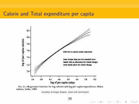
The graph plots the logarithm of calorie consumption against the logarithm of total household expenses per capital (outlay)

Graphs

The slope of this graph is about 0.35. Interpreting this graph: when total expenditure per capita increase by 1%, the consumption of calories increase by 0.35%

9

�

�

�



Graphs

The slope of this graph is about 0.35. Interpreting this graph: when total expenditure per capita increase by 1%, the consumption of calories increase by 0.35% This is an elasticity

10

�

�

�

�



Graphs

The slope of this graph is about 0.35. Interpreting this graph: when total expenditure per capita increase by 1%, the consumption of calories increase by 0.35% This is an elasticity The calories consumed increase with overall consumption: however, not 1 for 1: when total expenditure increase by 10%, the consumption of calories increases by about 3.5%. The Engel Curve

11

�

Why is the slope of the Engel curve less than 1?

What happens:

12

�

�


What happens: When they get a little more money, people increase the share of the budget going to other thing: elasticity of overall food expenditure is 0.7.

13

�

�

�


What happens: When they get a little more money, people increase the share of the budget going to other thing: elasticity of overall food expenditure is 0.7. When they spend more on food, they also buy more expensive calories (meat instead of cereals; rice instead of coarse cereals:

the elasticity is price per calorie is also about 0.35. table

graph

14

�

�

�

�

�


What happens: When they get a little more money, people increase the share of the budget going to other thing: elasticity of overall food expenditure is 0.7. When they spend more on food, they also buy more expensive calories (meat instead of cereals; rice instead of coarse cereals:

the elasticity is price per calorie is also about 0.35. table

graph

In summary: a poor household who is 10% richer spends about 7% more on food, and this extra spending is shared in half: half to get more calories, half to get more expensive (better tasting) calories. Even among very poor people, increase in economic well-being has a positive, but not huge impact on calories consumed.

15

�

Jensen and Miller: In search of a Giffen good

What is a Giffen good?

16

�


What is a Giffen good? A good whose consumption decreases when the price decreases.

17

�

�


What is a Giffen good? A good whose consumption decreases when the price decreases. Two effect when the price of a good decreases

18

�

�

�

�

�

�



An substitution effect: you want to consume more of this good because it has become less expensive than other goods. An income effect

Normal good: The income effect is positive (you consume more as income goes up) Inferior good: The income effect is negative (you consume less as income goes up)

19

�

�

�

�

�

�

�

�



An substitution effect: you want to consume more of this good because it has become less expensive than other goods. An income effect

Normal good: The income effect is positive (you consume more as income goes up) Inferior good: The income effect is negative (you consume less as income goes up)

In most cases, even for inferior goods the substitution effect will dominate, because most goods are only a small part of the budget. But for a staple food that constitutes a large part of the budget, a decrease in the price may have a large income effect: A giffen good is when the (negative) income effect is larger than the (positive) substitution effect 20

How to uncover a Giffen good?

21

�

�


First strategy: observe that, in China, in cities where the price of rice is higher, people consume more rice. Why did they conclude that this was not proof that rice was a Giffen good?

22

�

�

�


First strategy: observe that, in China, in cities where the price of rice is higher, people consume more rice. Why did they conclude that this was not proof that rice was a Giffen good? Second strategy. Conduct a randomized experiment:

23

�

�

�

�

�

�

�



Take a sample of households, and randomly chose a subsample of them. Distribute vouchers for reduced price of rice in Hunan, reduced price of wheat in Gangsu to the random subsample, for more than month supply Make sure that households do not exchange or trade them (otherwise it would be a pure income transfer, there would be no substitution). After 6 month, ask households detailed questions about their consumption of rice, wheat, and other stuff.

24

�

Main results

Hunan : when the price of rice decrease by 10%, rice consumption decrease by 2.5% (elasticity: -0.25).

25

�

�

Main results

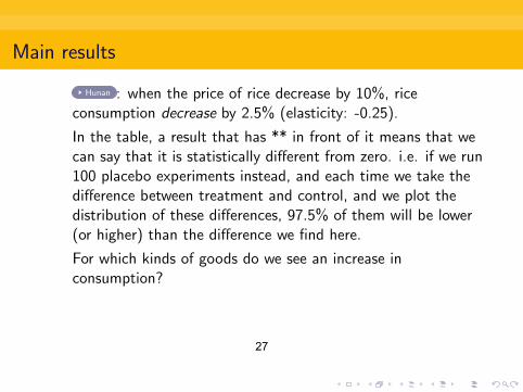
Hunan : when the price of rice decrease by 10%, rice consumption decrease by 2.5% (elasticity: -0.25). In the table, a result that has ** in front of it means that we can say that it is statistically different from zero. i.e. if we run 100 placebo experiments instead, and each time we take the difference between treatment and control, and we plot the distribution of these differences, 97.5% of them will be lower (or higher) than the difference we find here.

26

�

�

�

Main results

Hunan : when the price of rice decrease by 10%, rice consumption decrease by 2.5% (elasticity: -0.25). In the table, a result that has ** in front of it means that we can say that it is statistically different from zero. i.e. if we run 100 placebo experiments instead, and each time we take the difference between treatment and control, and we plot the distribution of these differences, 97.5% of them will be lower (or higher) than the difference we find here. For which kinds of goods do we see an increase in consumption?

27

�

�

�

�

Main results

Hunan : when the price of rice decrease by 10%, rice consumption decrease by 2.5% (elasticity: -0.25). In the table, a result that has ** in front of it means that we can say that it is statistically different from zero. i.e. if we run 100 placebo experiments instead, and each time we take the difference between treatment and control, and we plot the distribution of these differences, 97.5% of them will be lower (or higher) than the difference we find here. For which kinds of goods do we see an increase in consumption? What have households done?

28

�

�

�

�

�

Main results


Guansu : Elasticity is positive (not a Giffen good). 29

�

�

�

�

�

�

Main results


: Elasticity is positive (not a Giffen good). What explanation do they give for the different results?

Guansu

30

�

Implications for nutrition

Many countries use food price subsidies to encourage greater nutrition. For example India recently introduced nationally a subsidy scheme for rice in rice consuming regions.

31

�

�


Many countries use food price subsidies to encourage greater nutrition. For example India recently introduced nationally a subsidy scheme for rice in rice consuming regions. If households consume less rice and more shrimps, but shrimps are not very nutritious per dollar spent, the effect on calorie consumption of subsidizing rice may not be large, and it may even be negative.

32

�

�

�


Many countries use food price subsidies to encourage greater nutrition. For example India recently introduced nationally a subsidy scheme for rice in rice consuming regions. If households consume less rice and more shrimps, but shrimps are not very nutritious per dollar spent, the effect on calorie consumption of subsidizing rice may not be large, and it may even be negative. This is what they find in Hunan table.

33

�

�

�

�


Many countries use food price subsidies to encourage greater nutrition. For example India recently introduced nationally a subsidy scheme for rice in rice consuming regions. If households consume less rice and more shrimps, but shrimps are not very nutritious per dollar spent, the effect on calorie consumption of subsidizing rice may not be large, and it may even be negative. This is what they find in Hunan And this is true not only for calories but also other nutrients.

table.

34

�

�

�

�

�


Many countries use food price subsidies to encourage greater nutrition. For example India recently introduced nationally a subsidy scheme for rice in rice consuming regions. If households consume less rice and more shrimps, but shrimps are not very nutritious per dollar spent, the effect on calorie consumption of subsidizing rice may not be large, and it may even be negative. This is what they find in Hunan And this is true not only for calories but also other nutrients. What does this tell us about the effect income on calorie

table.

consumption in this population? 35

�

�

�

�

�

�


Many countries use food price subsidies to encourage greater nutrition. For example India recently introduced nationally a subsidy scheme for rice in rice consuming regions. If households consume less rice and more shrimps, but shrimps are not very nutritious per dollar spent, the effect on calorie consumption of subsidizing rice may not be large, and it may even be negative. This is what they find in Hunan And this is true not only for calories but also other nutrients. What does this tell us about the effect income on calorie

table.

consumption in this population? It must be negative. 36

�

Are the calorie Engel Curve overestimated?

How can we reconcile this result with the Engel curve we saw in India?

37

�

�


How can we reconcile this result with the Engel curve we saw in India? Note that we are comparing different households, not the same households as we give them more money. This may lead us to over-estimate the impact of well-being on calorie consumption

38

�

�

�

�


How can we reconcile this result with the Engel curve we saw in India? Note that we are comparing different households, not the same households as we give them more money. This may lead us to over-estimate the impact of well-being on calorie consumption

Those who eat more may be more productive and have more money (reverse causality) Those who have more income may be have different tastes, and would may be eat more even if they were poorer (for example, people who smoke may both eat less and earn less).

39

�

The Engel Curve over time

When we plot the Engel Curve over time in India (different years), we see that they fall down. graph

40

�

�


When we plot the Engel Curve over time in India (different years), we see that they fall down. With economic growth, household move up the Engel curve, but the Engel Curve falls: on balance the consumption of calories and all other nutrients has fallen in India over the last 25 years.

graph

41

�

�


When we plot the Engel Curve over time in India (different years), we see that they fall down. With economic growth, household move up the Engel curve, but the Engel Curve falls: on balance the consumption of calories and all other nutrients has fallen in India over the last 25 years.

graph

table

42

�

�

�


When we plot the Engel Curve over time in India (different years), we see that they fall down. With economic growth, household move up the Engel curve, but the Engel Curve falls: on balance the consumption of calories and all other nutrients has fallen in India over the last 25 years. What could be happening?

graph

table

43

�

Does eating more make people more productive?

Why are poor households not eating more and not seizing every available opportunity to eat more?

44

�

�


Why are poor households not eating more and not seizing every available opportunity to eat more? First hypothesis: may be they don’t need to eat as much

45

�

�

�

�


Why are poor households not eating more and not seizing every available opportunity to eat more? First hypothesis: may be they don’t need to eat as much Over time, in India, need for calories have gone down: less “backbreaking work”, fewer illnesses. Households in China where poor urban households.

46

�

�


A study by John Strauss: impact of calories on productivity in Sierra Leone (results do not come an experiment, but Strauss used the fact that people eat less when the price of food goes up).

Result Calories makes people more productive, but it looks like an inverted L-shape curve: it is highest for the poorest: when their calorie consumption increase by 1%, their productivity increase by 0.4%, and after that it goes down.

47

Take a sample of households, and randomly chose a subsampleof them.Distribute vouchers for reduced price of rice in Hunan, reducedprice of wheat in Gangsu to the random subsample, for morethan month supplyMake sure that households do not exchange or trade them(otherwise it would be a pure income transfer, there would beno substitution).After 6 month, ask households detailed questions about theirconsumption of rice, wheat, and other stuff.

�

�

�

�

�

�

�



48

What do the poor spend their money on? As a Share of Total Consumption

Alcohol/ Food Tobacco Education Health

Living on less than $1 a day Rural

Cote d'Ivoire 64.4% 2.7% 5.8% 2.2% Guatemala 65.9% 0.4% 0.1% 0.3% India - Udaipur 56.0% 5.0% 1.6% 5.1% Indonesia 66.1% 6.0% 6.3% 1.3% Mexico 49.6% 8.1% 6.9% 0.0% Nicaragua 57.3% 0.1% 2.3% 4.1% Pakistan 67.3% 3.1% 3.4% 3.4% Panama 67.8% 2.5% 4.0% Papua New Guinea 78.2% 4.1% 1.8% 0.3% Peru 71.8% 1.0% 1.9% 0.4% South Africa 71.5% 2.5% 0.8% 0.0% Timor Leste 76.5% 0.0% 0.8% 0.9% 49

Calorie and Total expenditure per capita

Courtesy of Angus Deaton. Used with permission.

50

Deaton and Subramanian, Table 1


51

How the food budget changes with wellbeing


52

Elasticity of consumption of various items with respect to price subsidy: Hunan

Table 4. Consumption Response to the Price Subsidy

HUNAN

Rice Other Cereal Fruit & Veg Meat Seafood Pulses Dairy Fats Food Out Non-Food %Subsidy(rice) -0.235* 0.397 -0.623*** 0.377 0.482** -0.791* -0.054 -0.567* 0.117 0.200 (0.140) (0.355) (0.227) (0.415) (0.230) (0.476) (0.069) (0.313) (0.347) (0.200) %ΔEarned 0.043*** -0.001 0.058*** 0.002 0.036 -0.052 -0.006 0.022 0.059 0.014 (0.014) (0.040) (0.021) (0.043) (0.022) (0.050) (0.004) (0.031) (0.044) (0.025) %ΔUnearned -0.044* -0.087 -0.018 0.076 -0.004 -0.037 -0.021 -0.007 0.020 0.089** (0.025) (0.065) (0.040) (0.071) (0.042) (0.075) (0.019) (0.055) (0.057) (0.038) %ΔPeople 0.89*** 0.46** 0.63*** 0.05 -0.07 0.48** 0.09 0.88*** -0.18 0.15 (0.08) (0.19) (0.11) (0.24) (0.10) (0.23) (0.05) (0.16) (0.18) (0.13) Constant 4.1*** 7.5*** -0.3 -5.7** -0.2 8.8*** 0.2 -8.3*** -3.5 -52.6*** (1.0) (2.5) (1.4) (2.8) (1.4) (3.0) (0.6) (2.1) (2.5) (1.5) Observations 1258 1258 1258 1258 1258 1258 1258 1258 1258 1258 R2 0.19 0.06 0.11 0.07 0.02 0.03 0.02 0.09 0.02 0.20

© Robert T. Jensen and Nolan H. Miller and the President and Fellows of HarvarCollege. All rights reserved. This content is excluded from our Creative Commons license. For more information, see http://ocw.mit.edu/fairuse.

53

http://ocw.mit.edu/fairuse

Wheat Other Cereal Fruit & Veg Meat Seafood Pulses Dairy Fats Food Out Non-Food %Subsidy(wheat) 0.353 -0.283 0.049 0.130 -0.017 0.240 0.282 0.507** 0.109 -0.021 (0.258) (0.335) (0.190) (0.299) (0.017) (0.320) (0.207) (0.251) (0.276) (0.180) %ΔEarned 0.079** -0.067 0.061** 0.085* 0.000 -0.047 -0.025 0.091*** 0.070 0.040 (0.036) (0.049) (0.027) (0.044) (0.000) (0.043) (0.029) (0.033) (0.043) (0.025) %ΔUnearned -0.017 0.130 0.046 0.314*** 0.025 0.012 0.108 -0.110 -0.077 0.229*** (0.092) (0.106) (0.077) (0.091) (0.025) (0.104) (0.073) (0.091) (0.097) (0.070) %ΔPeople 0.58*** 0.52* 1.01*** -0.10 -0.01 0.44** 0.10 0.66 0.00 -0.04 (0.22) (0.29) (0.15) (0.28) (0.01) (0.18) (0.12) (0.15) (0.19) (0.19) Constant -26.1*** 23.8*** 11.0*** 2.4 -0.2 6.0** -3.4* 7.2 7.5*** -38.2*** (2.3) (2.8) (1.6) (2.5) (0.2) (2.6) (1.9) (2.1) (2.4) (1.4) Observations 1269 1269 1269 1269 1269 1269 1269 1269 1269 1269 R2 0.08 0.06 0.07 0.05 0.03 0.06 0.03 0.07 0.05 0.17

Elasticity of consumption of various items with respect to price subsidy: Gansu

© Robert T. Jensen and Nolan H. Miller and the President and Fellows of Harvard College. All rights reserved. This content is excluded from our Creative Commons license. For more information, see http://ocw.mit.edu/fairuse.

54


Calories and rice price subsidy Table 2. Calorie Response to the Price Subsidy

HUNAN GANSU

(1) (2)

(3)

(4)

(5)

(6)

(7)

(8) (9) (10)

Full Sample

(Calories)

Below Median

(Calories)

Above Median

(Calories)

Bottom Quartile

(Calories)

Full

Sample (Protein)

Full

Sample (Calories)

Below Median

(Calories)

Above Median

(Calories)

Bottom Quartile

(Calories)

Full

Sample (Protein)

%Subsidy(rice/wheat) -0.206* -0.042 -0.339** 0.004 -0.096 0.154 0.169 0.132 0.070 0.091 (0.108) (0.144) (0.164) (0.207) (0.133) (0.100) (0.143) (0.138) (0.261) (0.112)

%ΔEarned 0.031*** 0.026* 0.036** 0.037* 0.040*** 0.028** 0.027 0.029 0.053 0.017 (0.011) (0.014) (0.018) (0.021) (0.013) (0.014) (0.021) (0.019) (0.034) (0.016)

%ΔUnearned -0.022 -0.025 -0.023 -0.037 -0.010 0.046 0.020 0.071* 0.101 0.069 (0.020) (0.027) (0.028) (0.034) (0.023) (0.035) (0.056) (0.043) (0.119) (0.033)

%ΔPeople 0.94*** 1.07*** 0.80 1.04*** 0.93*** 0.91*** 1.01*** 0.81*** 1.08*** 0.88***

(0.07) (0.08) (0.11) (0.10) (0.07) (0.08) (0.10) (0.12) (0.13) (0.09) Constant 9 1.6 0.5*** 2.8* 0.8 -1.9 0.1 -3.9 0.6 -4.0

(0.8) (1.1) (1.1) (1.5) (0.9) (0.8) (1.1) (1.1) (1.7) (0.9)

Observations 1258 633 625 317 1258 1269 634 635 320 1269R2 0.26 0.34 0.21 0.39 0.20 0.18 0.23 0.15 0.29 0.16 Notes: Regressions include county*time fixed-effects. The dependent variable in columns 1-4 and 6-9 is the arc percent change in household caloric intake and in columns 5 and 10 it is the arc percent change in household protein consumption. Standard errors clustered at the household level. %Subsidy (rice/wheat) is the rice or wheat price subsidy, measured as a percentage of the average price. %ΔEarned is the arc percent change in the household earnings from work; %ΔHH Unearned is the arc percent change in the household income from unearned sources (government payments, pensions, remittances, rent and interest from assets); %ΔPeople is the arc percent change in the number of people living in the household. *Significant at 10 percent level. **Significant at 5 percent level. ***Significant at 1 percent level.


55


Elasticity of consumption of various items with respect to price subsidy: Hunan

Table 4. Consumption Response to the Price Subsidy

HUNAN

Rice Other Cereal Fruit & Veg Meat Seafood Pulses Dairy Fats Food Out Non-Food %Subsidy(rice) -0.235* 0.397 -0.623*** 0.377 0.482** -0.791* -0.054 -0.567* 0.117 0.200 (0.140) (0.355) (0.227) (0.415) (0.230) (0.476) (0.069) (0.313) (0.347) (0.200) %ΔEarned 0.043*** -0.001 0.058*** 0.002 0.036 -0.052 -0.006 0.022 0.059 0.014 (0.014) (0.040) (0.021) (0.043) (0.022) (0.050) (0.004) (0.031) (0.044) (0.025) %ΔUnearned -0.044* -0.087 -0.018 0.076 -0.004 -0.037 -0.021 -0.007 0.020 0.089** (0.025) (0.065) (0.040) (0.071) (0.042) (0.075) (0.019) (0.055) (0.057) (0.038) %ΔPeople 0.89*** 0.46** 0.63*** 0.05 -0.07 0.48** 0.09 0.88*** -0.18 0.15 (0.08) (0.19) (0.11) (0.24) (0.10) (0.23) (0.05) (0.16) (0.18) (0.13) Constant 4.1*** 7.5*** -0.3 -5.7** -0.2 8.8*** 0.2 -8.3*** -3.5 -52.6*** (1.0) (2.5) (1.4) (2.8) (1.4) (3.0) (0.6) (2.1) (2.5) (1.5) Observations 1258 1258 1258 1258 1258 1258 1258 1258 1258 1258 R2 0.19 0.06 0.11 0.07 0.02 0.03 0.02 0.09 0.02 0.20

56



Fractions of the Population Living in Householdswith per Capita Calorie Consumption below 2,100

Urban and 2,400 Rural

Year Round Rural Urban All India

1983 38 66.1 60.5 64.8

1987-8 43 65.9 57.1 63.9

1993-4 50 71.1 58.1 67.8

1999-0 55 74.2 58.2 70.1

2004-5 61 79.8 63.9 75.8

Source: Authors' calculations based on NSS data.

Figure by MIT OpenCourseWare.

57

John Strauss: Nutrition and Farm Productivity

��8QLYHUVLW\�RI�&KLFDJR�3UHVV� $OO�ULJKWV�UHVHUYHG��ThisFRQWHQW�LV�H[FOXGHG�IURP�RXU�&UHDWLYH�&RPPRQV�OLFHQVH�)RU�PRUH�LQIRUPDWLRQ��VHH�KWWS��RFZ�PLW�HGX�IDLUXVH�

58


MIT OpenCourseWare http://ocw.mit.edu

14.73 The Challenge of World Poverty Spring 2011

For information about citing these materials or our Terms of Use, visit: http://ocw.mit.edu/terms.

http://ocw.mit.edu

http://ocw.mit.edu/terms

Lecture 5: Is there a nutrition-based poverty trap?

Documents

Transcript of Lecture 5: Is there a nutrition-based poverty trap?