Lecture # 5 Histogram Matching & Spatial Filteringbiomisa.org/uploads/2016/02/Lect-5.pdf ·...
54
1 Digital Image Processing Lecture # 5 Histogram Matching & Spatial Filtering
Transcript of Lecture # 5 Histogram Matching & Spatial Filteringbiomisa.org/uploads/2016/02/Lect-5.pdf ·...
1
Digital Image Processing
Lecture # 5 Histogram Matching & Spatial Filtering
2
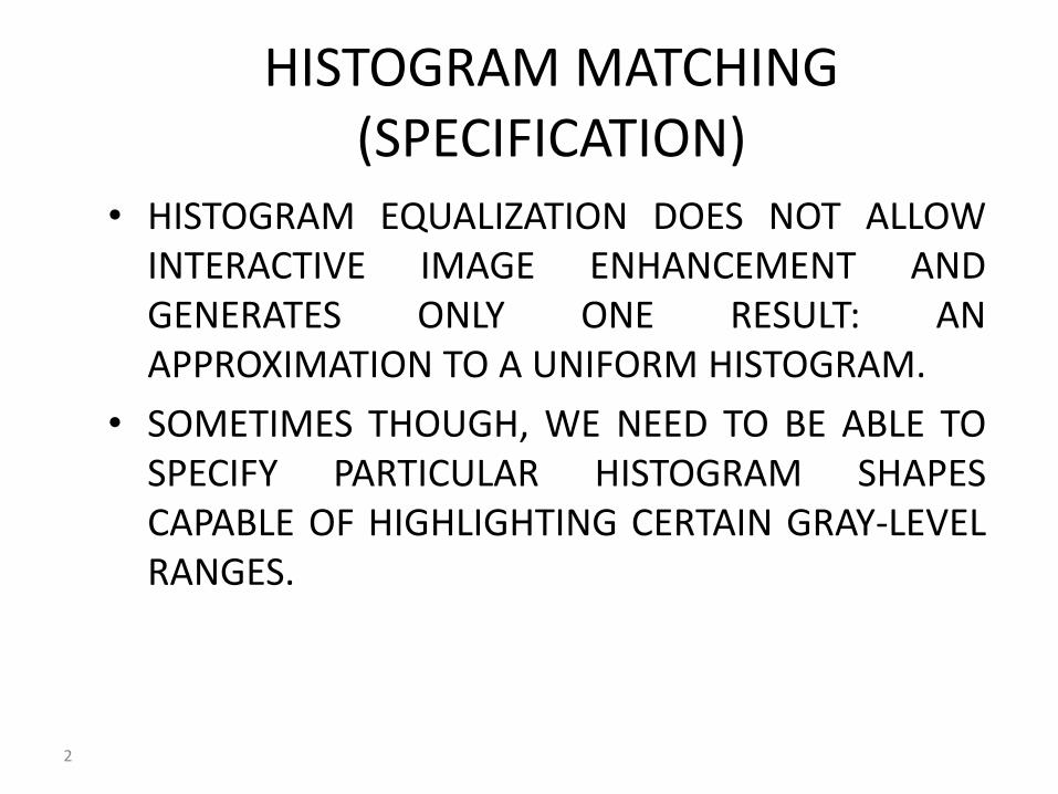
HISTOGRAM MATCHING (SPECIFICATION)
• HISTOGRAM EQUALIZATION DOES NOT ALLOW INTERACTIVE IMAGE ENHANCEMENT AND GENERATES ONLY ONE RESULT: AN APPROXIMATION TO A UNIFORM HISTOGRAM.
• SOMETIMES THOUGH, WE NEED TO BE ABLE TO SPECIFY PARTICULAR HISTOGRAM SHAPES CAPABLE OF HIGHLIGHTING CERTAIN GRAY-LEVEL RANGES.
3
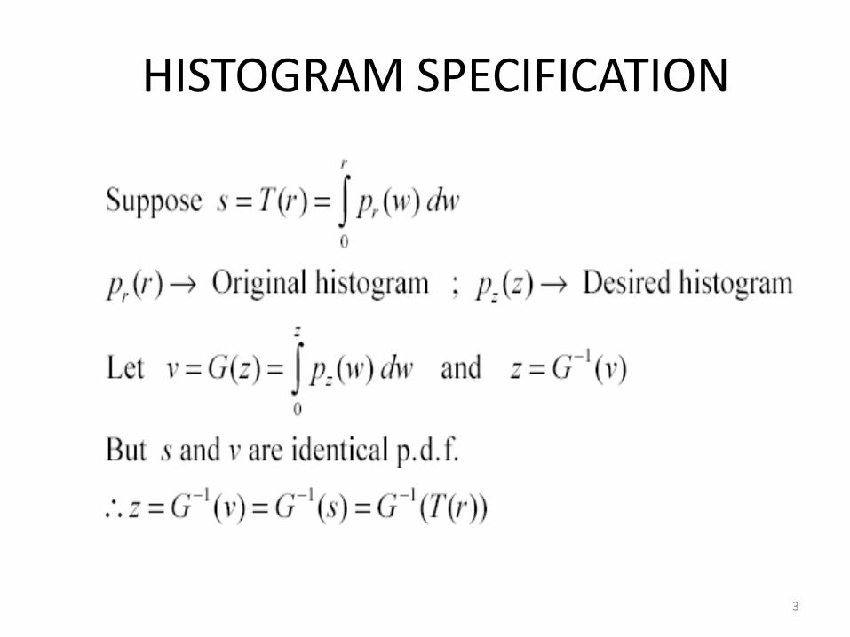
HISTOGRAM SPECIFICATION
4
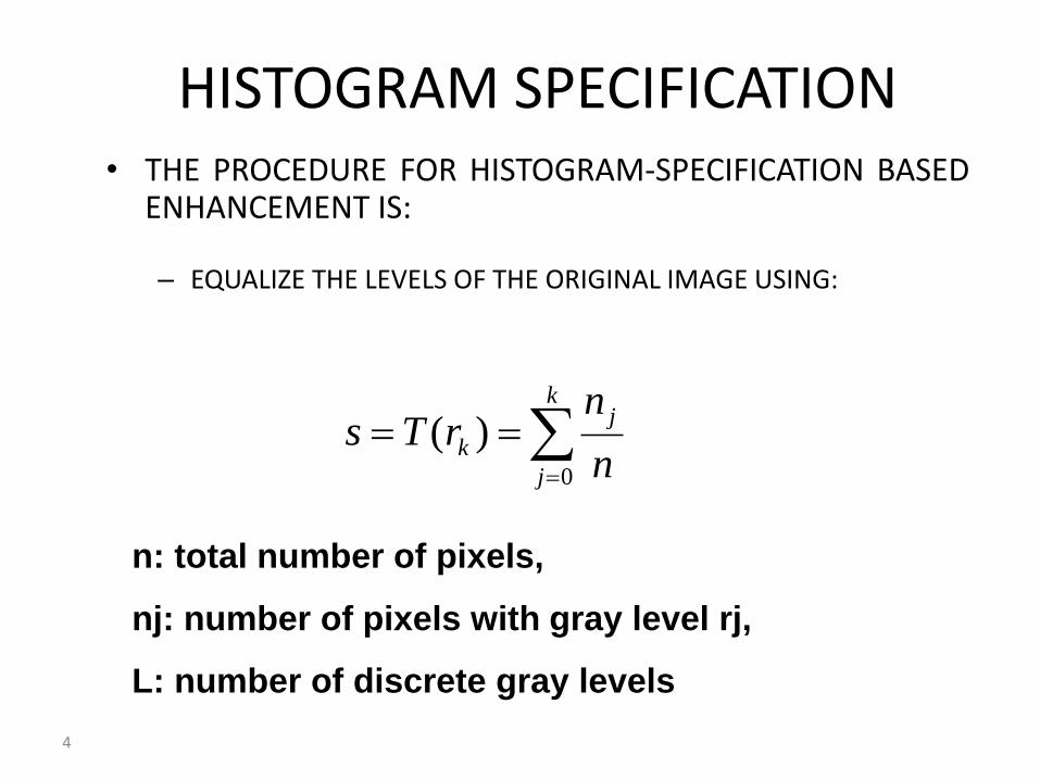
HISTOGRAM SPECIFICATION • THE PROCEDURE FOR HISTOGRAM-SPECIFICATION BASED
ENHANCEMENT IS:
– EQUALIZE THE LEVELS OF THE ORIGINAL IMAGE USING:
k
j
j
kn
nrTs
0
)(
n: total number of pixels,
nj: number of pixels with gray level rj,
L: number of discrete gray levels
5
HISTOGRAM SPECIFICATION
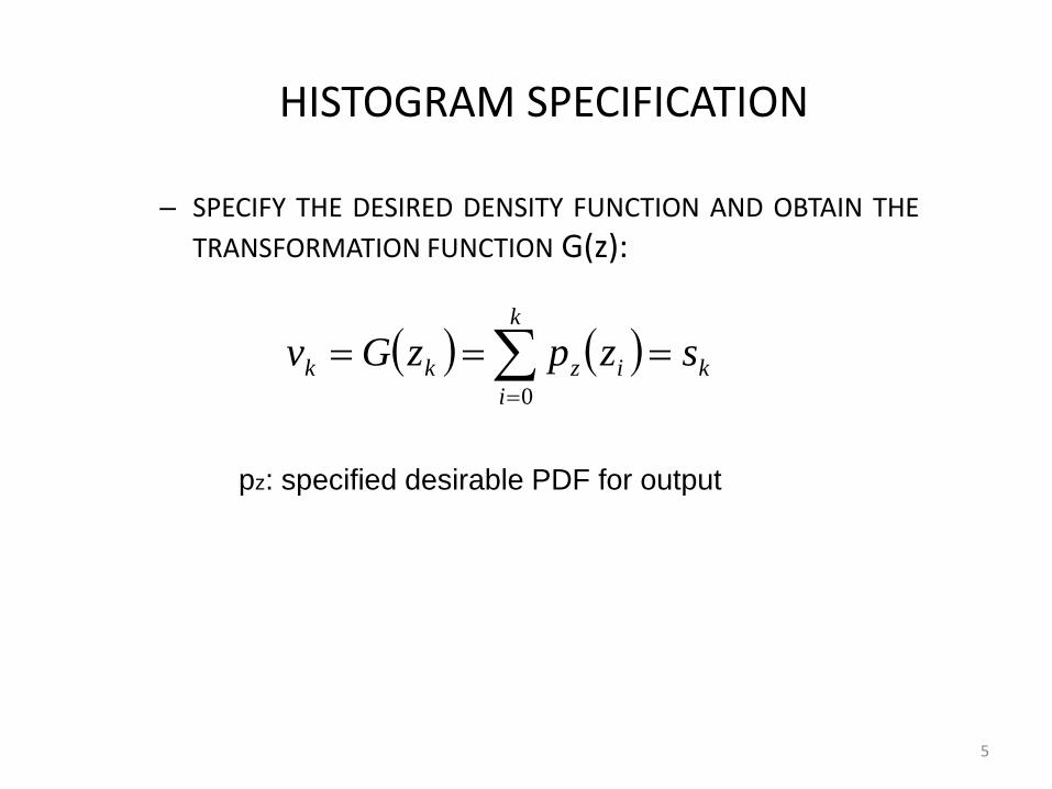
– SPECIFY THE DESIRED DENSITY FUNCTION AND OBTAIN THE
TRANSFORMATION FUNCTION G(z):
pz: specified desirable PDF for output
ki
k
i
zkk szpzGv 0
6
HISTOGRAM SPECIFICATION
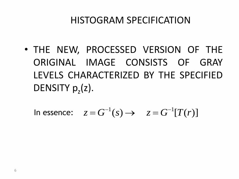
• THE NEW, PROCESSED VERSION OF THE ORIGINAL IMAGE CONSISTS OF GRAY LEVELS CHARACTERIZED BY THE SPECIFIED DENSITY pz(z).
)]([ )( 11 rTGzsGz In essence:
7
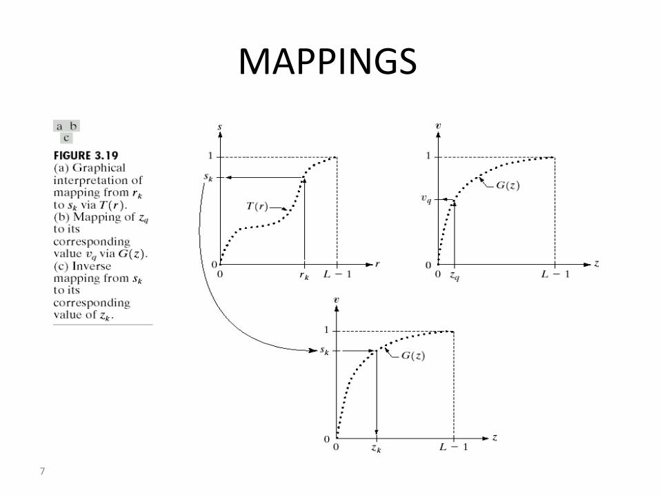
MAPPINGS
8
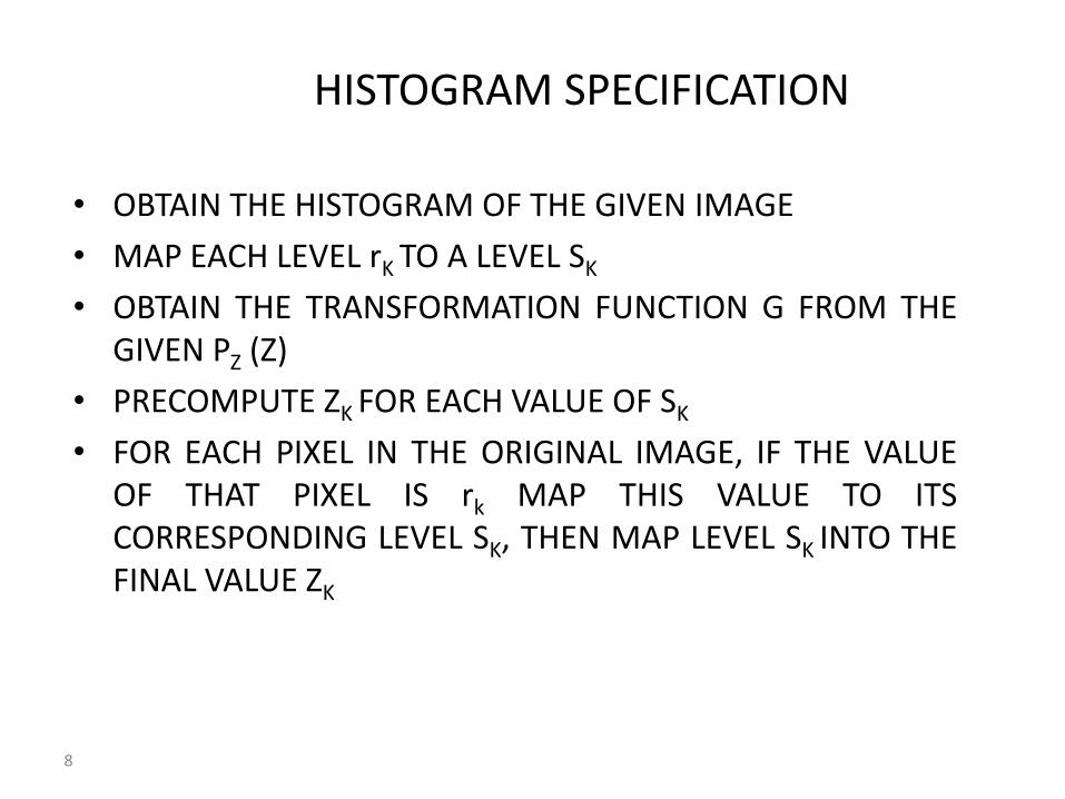
HISTOGRAM SPECIFICATION
• OBTAIN THE HISTOGRAM OF THE GIVEN IMAGE
• MAP EACH LEVEL rK TO A LEVEL SK
• OBTAIN THE TRANSFORMATION FUNCTION G FROM THE GIVEN PZ (Z)
• PRECOMPUTE ZK FOR EACH VALUE OF SK
• FOR EACH PIXEL IN THE ORIGINAL IMAGE, IF THE VALUE OF THAT PIXEL IS rk MAP THIS VALUE TO ITS CORRESPONDING LEVEL SK, THEN MAP LEVEL SK INTO THE FINAL VALUE ZK
9
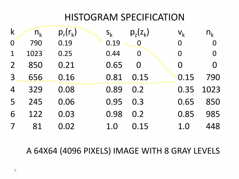
HISTOGRAM SPECIFICATION
k nk pr(rk) sk pz(zk) vk nk
0 790 0.19 0.19 0 0 0
1 1023 0.25 0.44 0 0 0
2 850 0.21 0.65 0 0 0
3 656 0.16 0.81 0.15 0.15 790
4 329 0.08 0.89 0.2 0.35 1023
5 245 0.06 0.95 0.3 0.65 850
6 122 0.03 0.98 0.2 0.85 985
7 81 0.02 1.0 0.15 1.0 448
A 64X64 (4096 PIXELS) IMAGE WITH 8 GRAY LEVELS
10
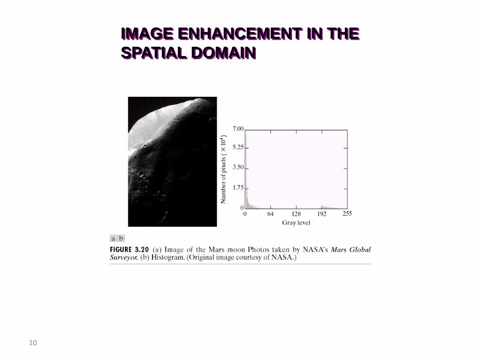
IMAGE ENHANCEMENT IN THE
SPATIAL DOMAIN
11
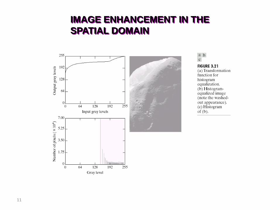
IMAGE ENHANCEMENT IN THE
SPATIAL DOMAIN
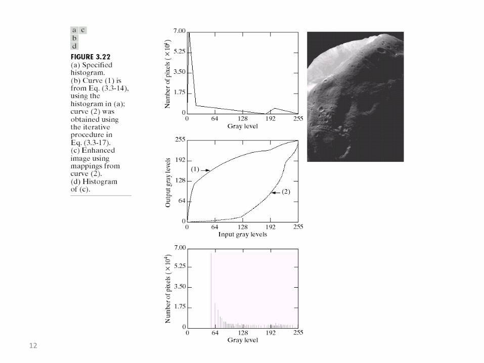
12
13
GLOBAL/LOCAL HISTOGRAM EQUALIZATION
• IT MAY BE NECESSARY TO ENHANCE DETAILS OVER SMALL AREAS IN THE IMAGE
• THE NUMBER OF PIXELS IN THESE AREAS MAY HAVE NEGLIGIBLE INFLUENCE ON THE COMPUTATION OF A GLOBAL TRANSFORMATION WHOSE SHAPE DOES NOT NECESSARILY GUARANTEE THE DESIRED LOCAL ENHANCEMENT
• DEVISE TRANSFORMATION FUNCTIONS BASED ON THE GRAY LEVEL DISTRIBUTION IN THE NEIGHBORHOOD OF EVERY PIXEL IN THE IMAGE
• THE PROCEDURE IS: – DEFINE A SQUARE (OR RECTANGULAR) NEIGHBORHOOD AND MOVE THE
CENTER OF THIS AREA FROM PIXEL TO PIXEL. – AT EACH LOCATION, THE HISTOGRAM OF THE POINTS IN THE
NEIGHBORHOOD IS COMPUTED AND EITHER A HISTOGRAM EQUALIZATION OR HISTOGRAM SPECIFICATION TRANSFORMATION FUNCTION IS OBTAINED.
– THIS FUNCTION IS FINALLY USED TO MAP THE GRAY LEVEL OF THE PIXEL CENTERED IN THE NEIGHBORHOOD.
– THE CENTER IS THEN MOVED TO AN ADJACENT PIXEL LOCATION AND THE PROCEDURE IS REPEATED.
14
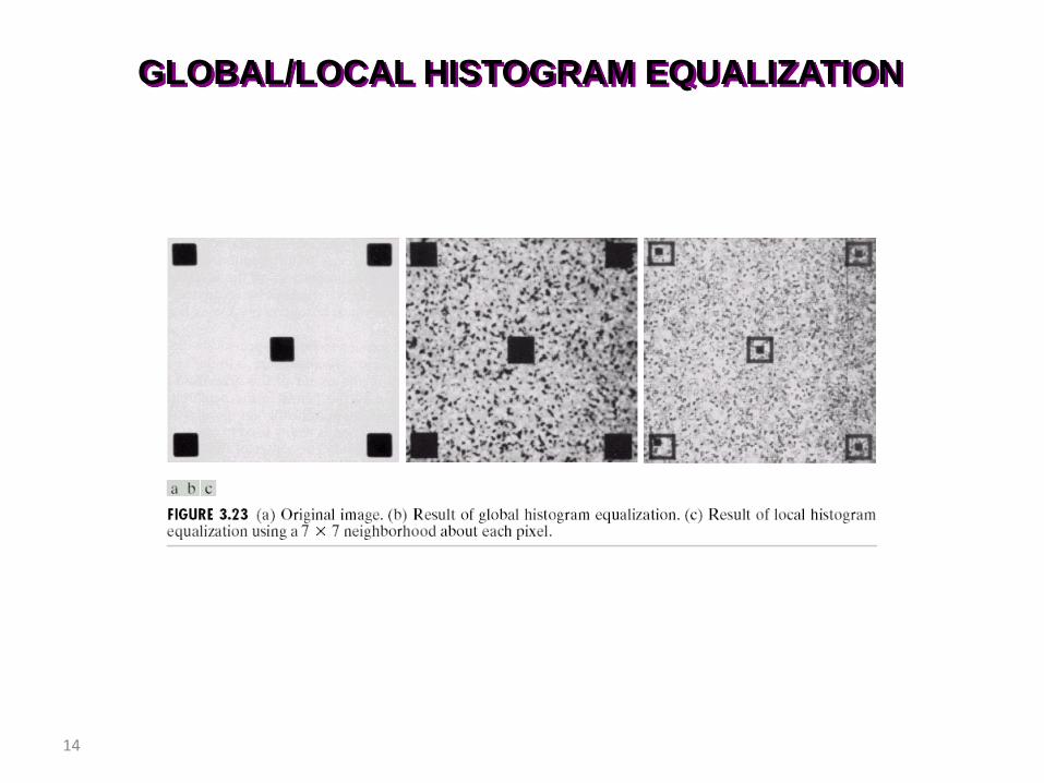
GLOBAL/LOCAL HISTOGRAM EQUALIZATION
15
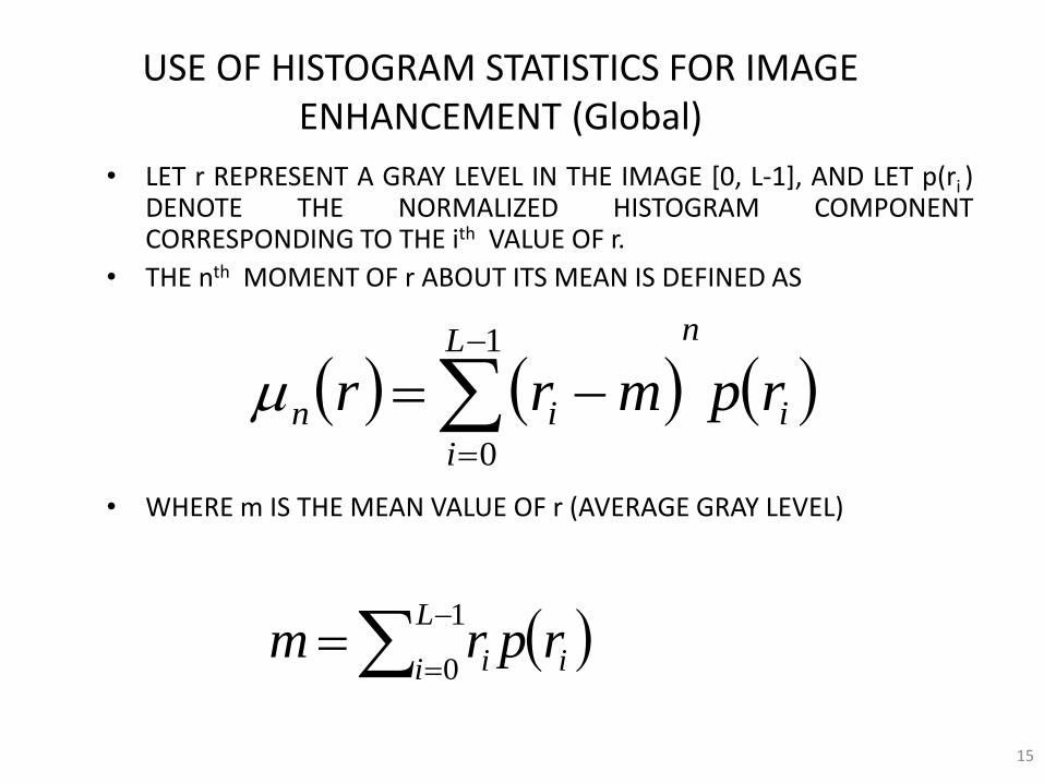
USE OF HISTOGRAM STATISTICS FOR IMAGE ENHANCEMENT (Global)
• LET r REPRESENT A GRAY LEVEL IN THE IMAGE [0, L-1], AND LET p(ri ) DENOTE THE NORMALIZED HISTOGRAM COMPONENT CORRESPONDING TO THE ith VALUE OF r.
• THE nth MOMENT OF r ABOUT ITS MEAN IS DEFINED AS
• WHERE m IS THE MEAN VALUE OF r (AVERAGE GRAY LEVEL)
i
nL
i
in rpmrr
1
0
iL
i i rprm
1
0
16
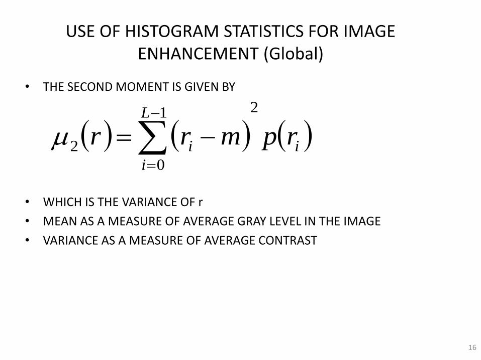
USE OF HISTOGRAM STATISTICS FOR IMAGE ENHANCEMENT (Global)
• THE SECOND MOMENT IS GIVEN BY
• WHICH IS THE VARIANCE OF r
• MEAN AS A MEASURE OF AVERAGE GRAY LEVEL IN THE IMAGE
• VARIANCE AS A MEASURE OF AVERAGE CONTRAST
i
L
i
i rpmrr
21
0
2
17
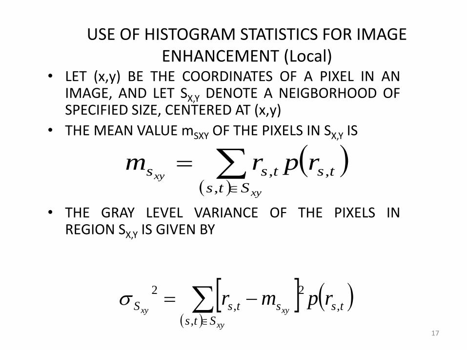
USE OF HISTOGRAM STATISTICS FOR IMAGE ENHANCEMENT (Local)
• LET (x,y) BE THE COORDINATES OF A PIXEL IN AN IMAGE, AND LET SX,Y DENOTE A NEIGBORHOOD OF SPECIFIED SIZE, CENTERED AT (x,y)
• THE MEAN VALUE mSXY OF THE PIXELS IN SX,Y IS
• THE GRAY LEVEL VARIANCE OF THE PIXELS IN REGION SX,Y IS GIVEN BY
ts
Sts
tss rprmxy
xy ,
,
,
ts
Sts
stsS rpmrxy
xyxy ,
,
2
,
2
18
USE OF HISTOGRAM STATISTICS FOR IMAGE ENHANCEMENT
• THE GLOBAL MEAN AND VARIANCE ARE MEASURED OVER AN ENTIRE IMAGE AND ARE USEFUL FOR GROSS ADJUSTMENTS OF OVERALL INTENSITY AND CONTRAST.
• A USE OF THESE MEASURES IN LOCAL ENHANCEMENT IS, WHERE THE LOCAL MEAN AND VARIANCE ARE USED AS THE BASIS FOR MAKING CHANGES THAT DEPEND ON IMAGE CHARACTERISTICS IN A PREDEFINED REGION ABOUT EACH PIXEL IN THE IMAGE.
19
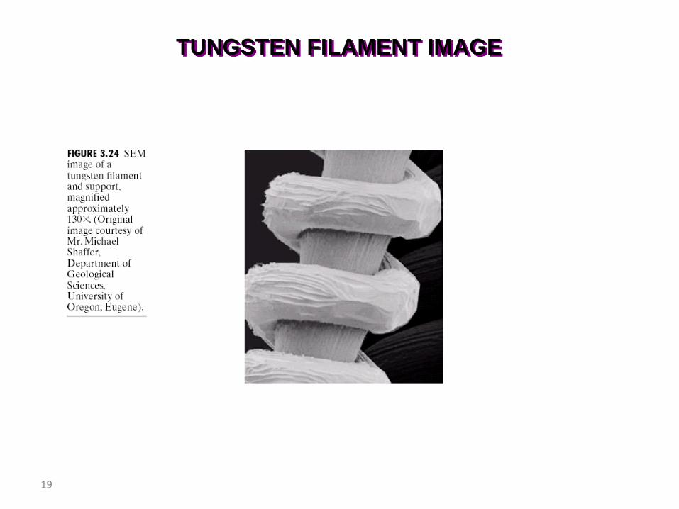
TUNGSTEN FILAMENT IMAGE
20
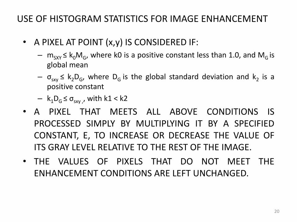
USE OF HISTOGRAM STATISTICS FOR IMAGE ENHANCEMENT
• A PIXEL AT POINT (x,y) IS CONSIDERED IF: – mSXY ≤ k0MG, where k0 is a positive constant less than 1.0, and MG is
global mean
– σsxy ≤ k2DG, where DG is the global standard deviation and k2 is a positive constant
– k1DG ≤ σsxy ,, with k1 < k2
• A PIXEL THAT MEETS ALL ABOVE CONDITIONS IS PROCESSED SIMPLY BY MULTIPLYING IT BY A SPECIFIED CONSTANT, E, TO INCREASE OR DECREASE THE VALUE OF ITS GRAY LEVEL RELATIVE TO THE REST OF THE IMAGE.
• THE VALUES OF PIXELS THAT DO NOT MEET THE ENHANCEMENT CONDITIONS ARE LEFT UNCHANGED.
21
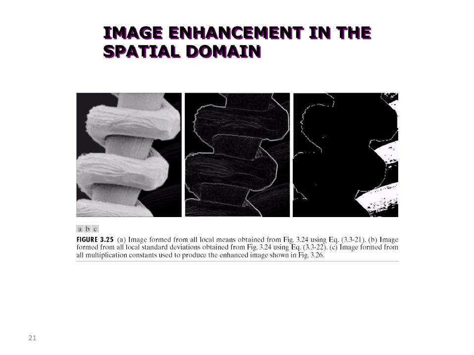
IMAGE ENHANCEMENT IN THE SPATIAL DOMAIN
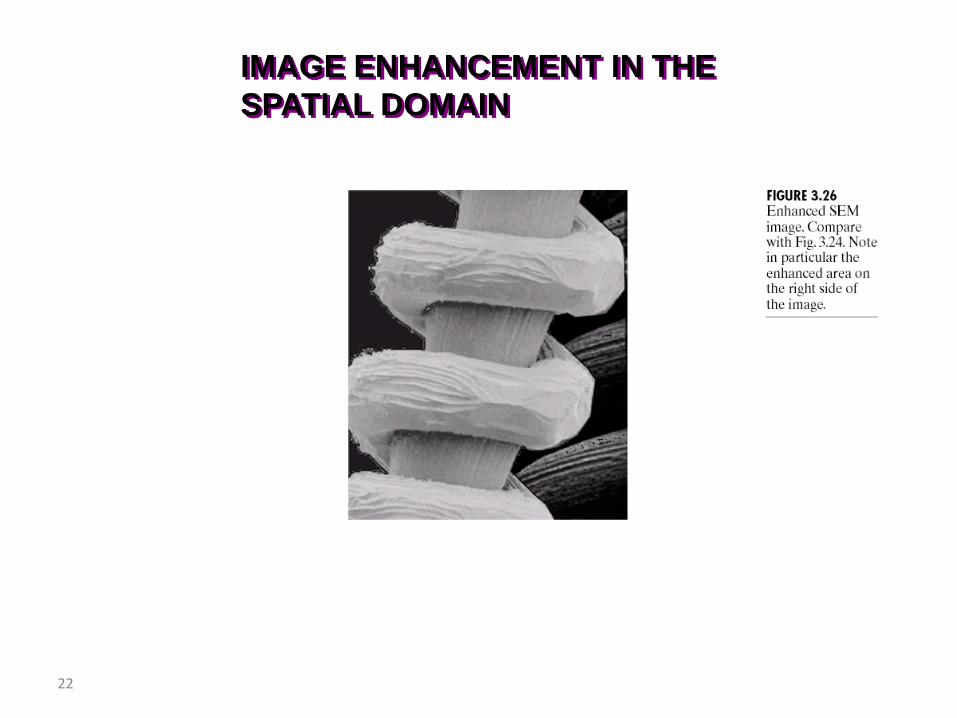
22
IMAGE ENHANCEMENT IN THE
SPATIAL DOMAIN
Spatial Filtering
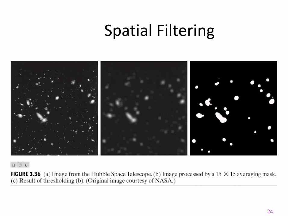
24
Spatial Filtering
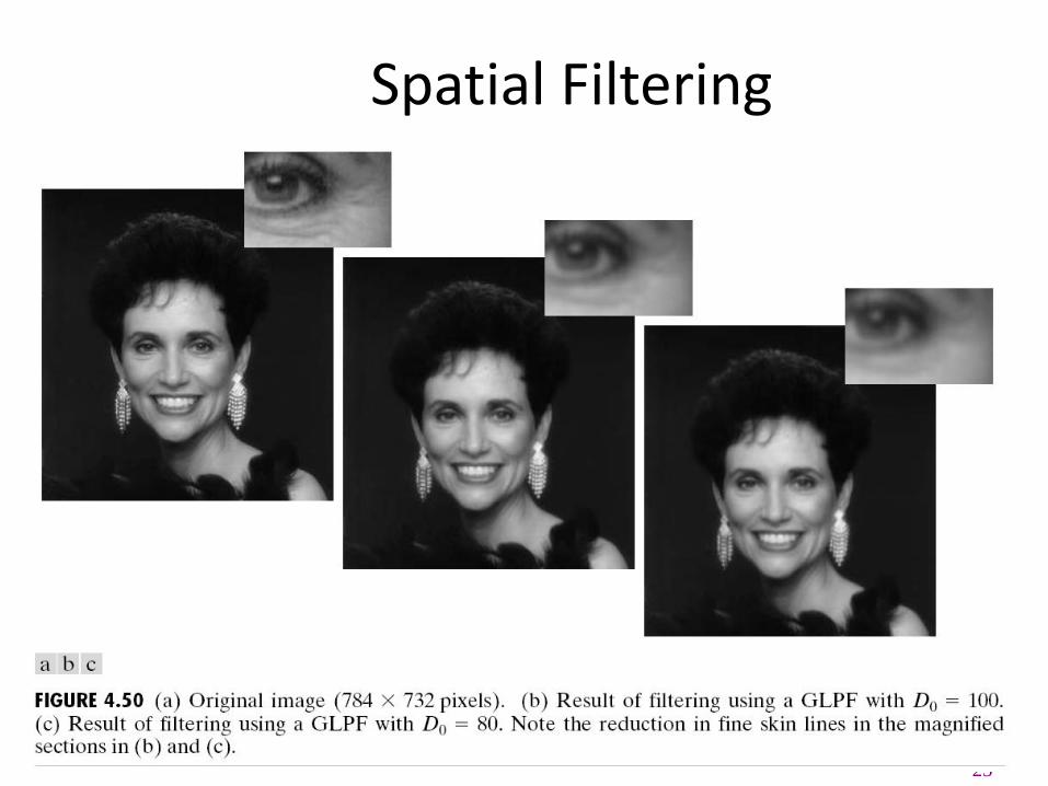
25
Spatial Filtering
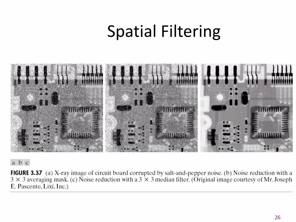
26
Spatial Filtering
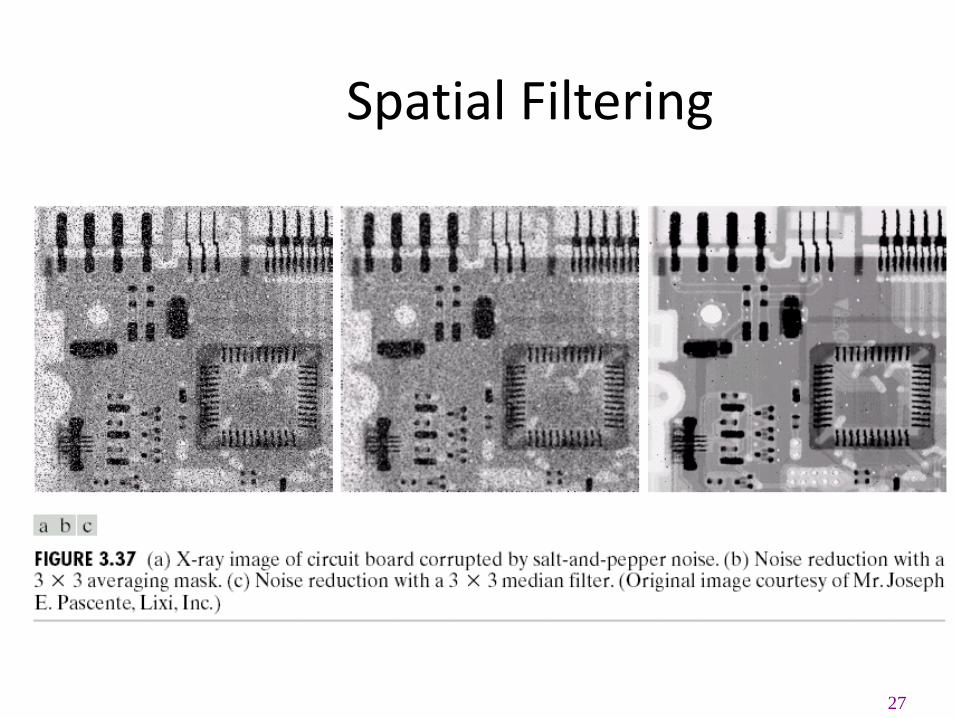
27
Spatial Filtering
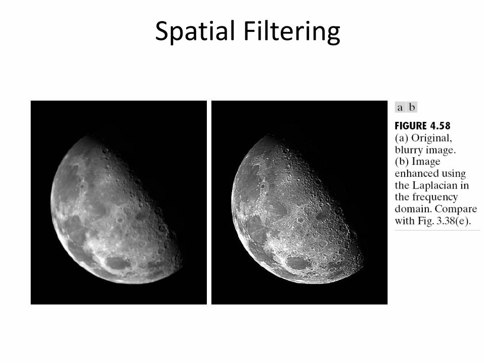
Spatial Filtering
29
Spatial Filtering: Basics
The output intensity value at (x,y) depends not only on the input intensity value at (x,y) but also on the specified number of neighboring intensity values around (x,y)
Spatial masks (also called window, filter, kernel, template) are used and convolved over the entire image for local enhancement (spatial filtering)
The size of the masks determines the number of neighboring pixels which influence the output value at (x,y)
The values (coefficients) of the mask determine the nature and properties of enhancing technique
30
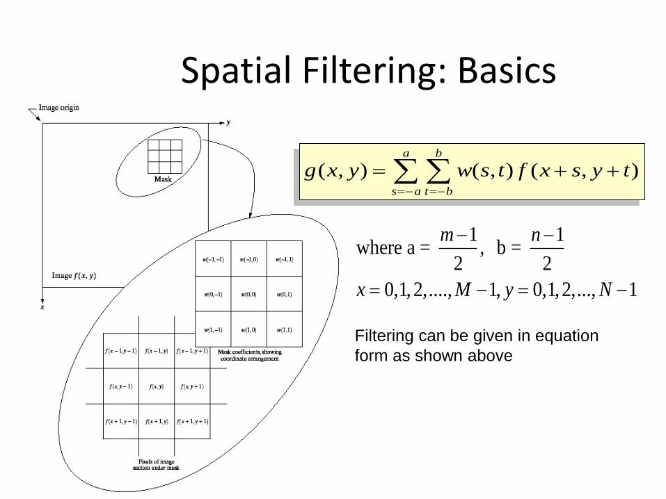
Spatial Filtering: Basics
1 1where a = , b =
2 2
0,1,2,...., 1, 0,1,2,..., 1
m n
x M y N
( , ) ( , ) ( , )a b
s a t b
g x y w s t f x s y t
Filtering can be given in equation
form as shown above
31
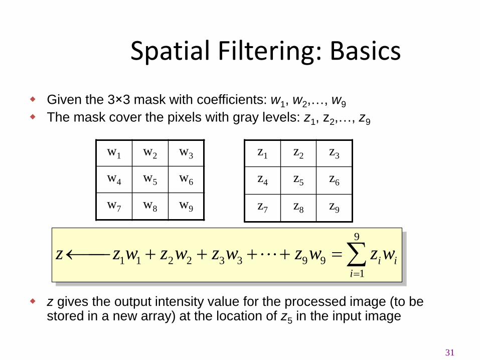
Spatial Filtering: Basics
Given the 3×3 mask with coefficients: w1, w2,…, w9
The mask cover the pixels with gray levels: z1, z2,…, z9
z gives the output intensity value for the processed image (to be stored in a new array) at the location of z5 in the input image
z1 z2 z3
z4 z5 z6
z7 z8 z9
9
1 1 2 2 3 3 9 9
1
i i
i
z z w z w z w z w z w
w1 w2 w3
w4 w5 w6
w7 w8 w9
34
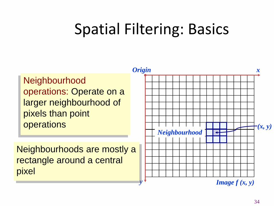
Spatial Filtering: Basics
Neighbourhood
operations: Operate on a
larger neighbourhood of
pixels than point
operations
Origin x
y Image f (x, y)
(x, y) Neighbourhood
Neighbourhoods are mostly a
rectangle around a central
pixel
35
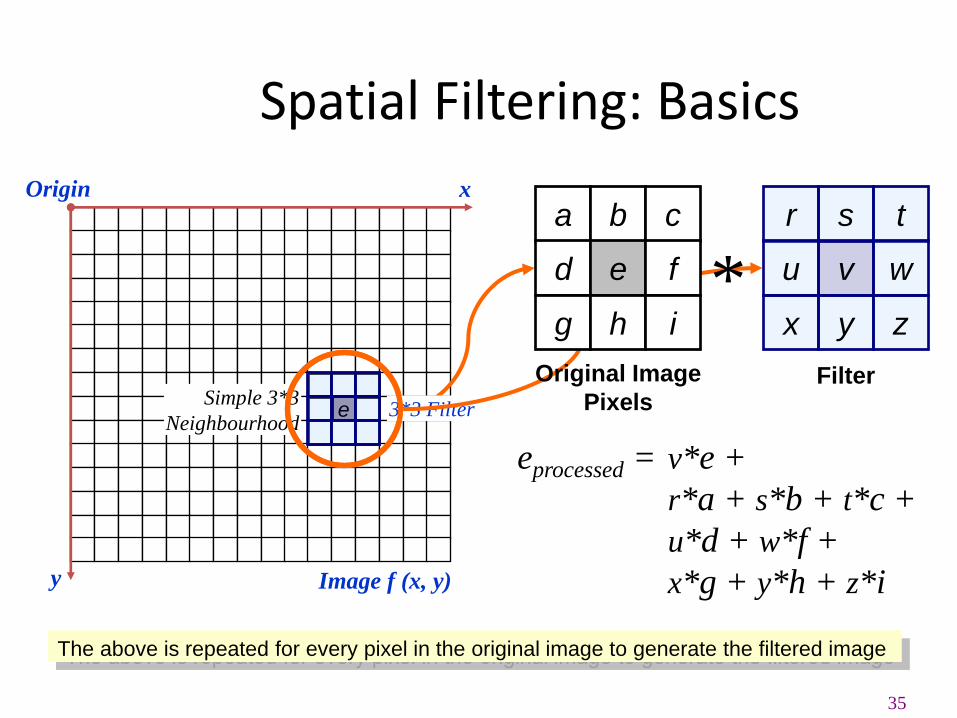
Spatial Filtering: Basics
r s t
u v w
x y z
Origin x
y Image f (x, y)
eprocessed = v*e +
r*a + s*b + t*c +
u*d + w*f +
x*g + y*h + z*i
Filter Simple 3*3
Neighbourhood e 3*3 Filter
a b c
d e f
g h i
Original Image
Pixels
*
The above is repeated for every pixel in the original image to generate the filtered image
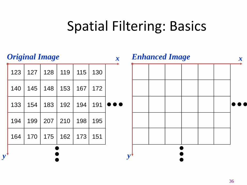
36
Spatial Filtering: Basics
123 127 128 119 115 130
140 145 148 153 167 172
133 154 183 192 194 191
194 199 207 210 198 195
164 170 175 162 173 151
Original Image x
y
Enhanced Image x
y
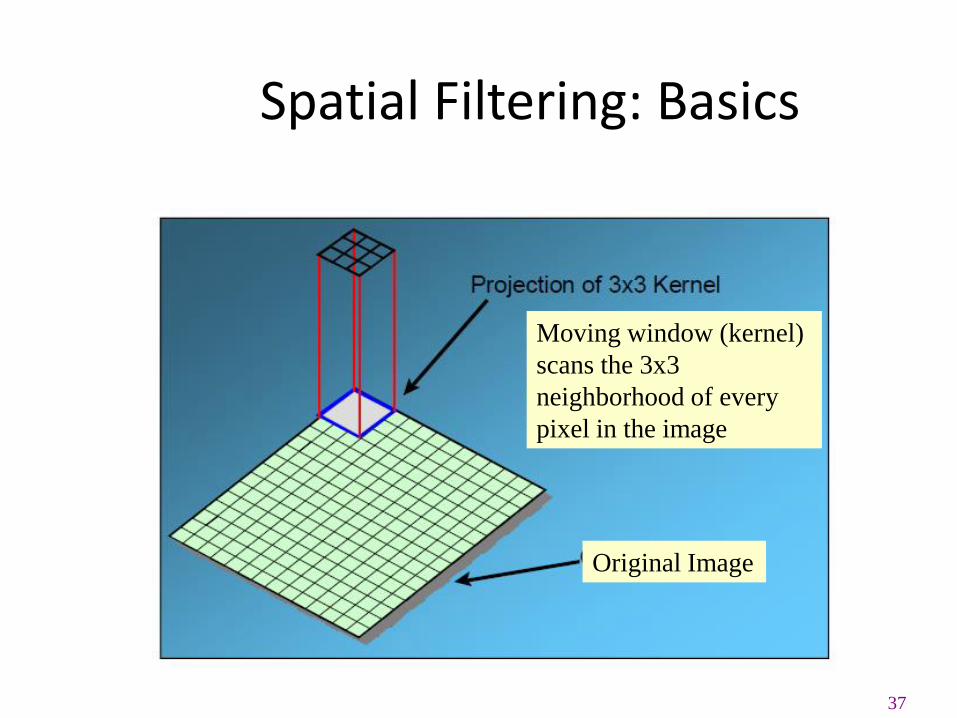
37
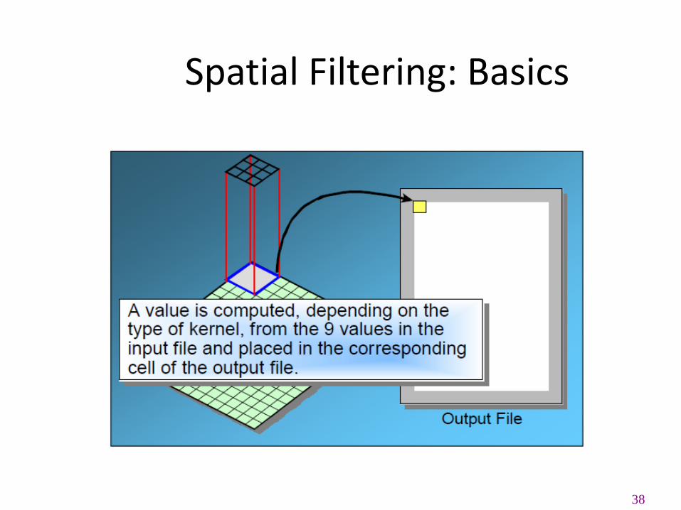
Spatial Filtering: Basics
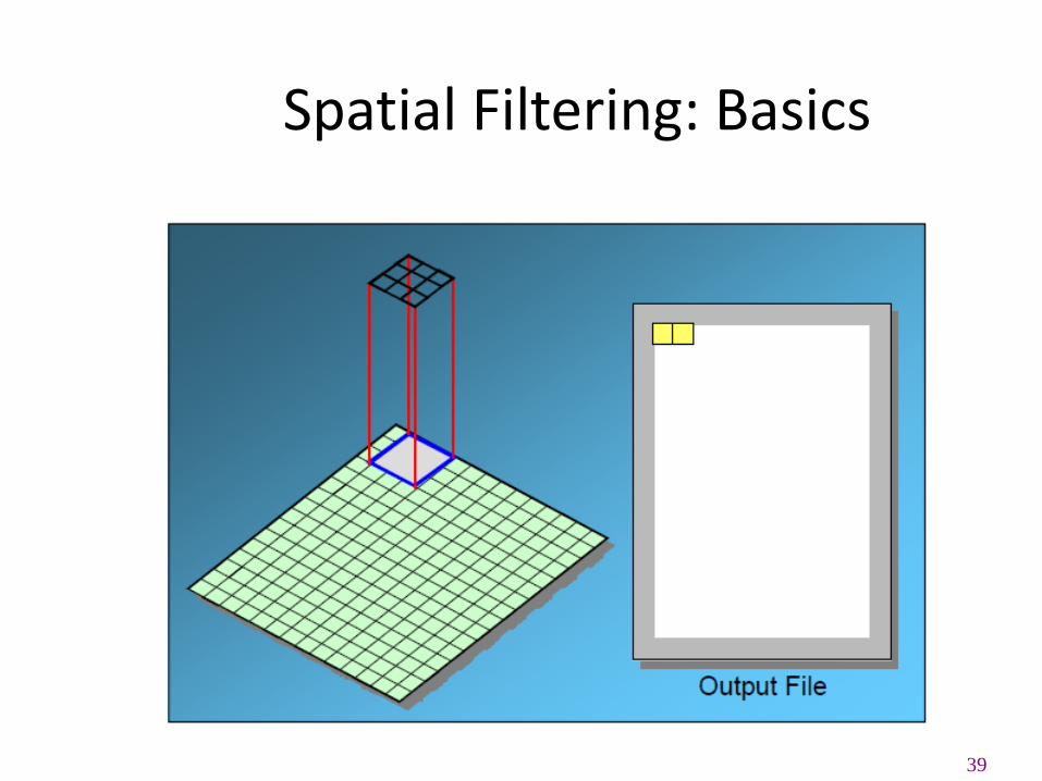
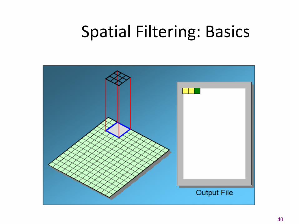
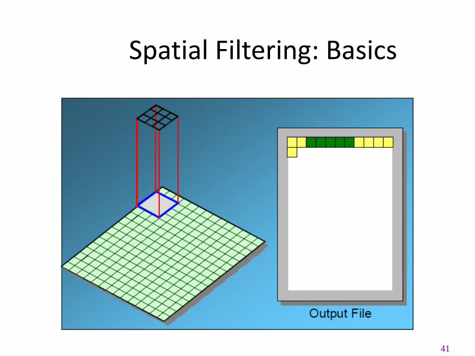
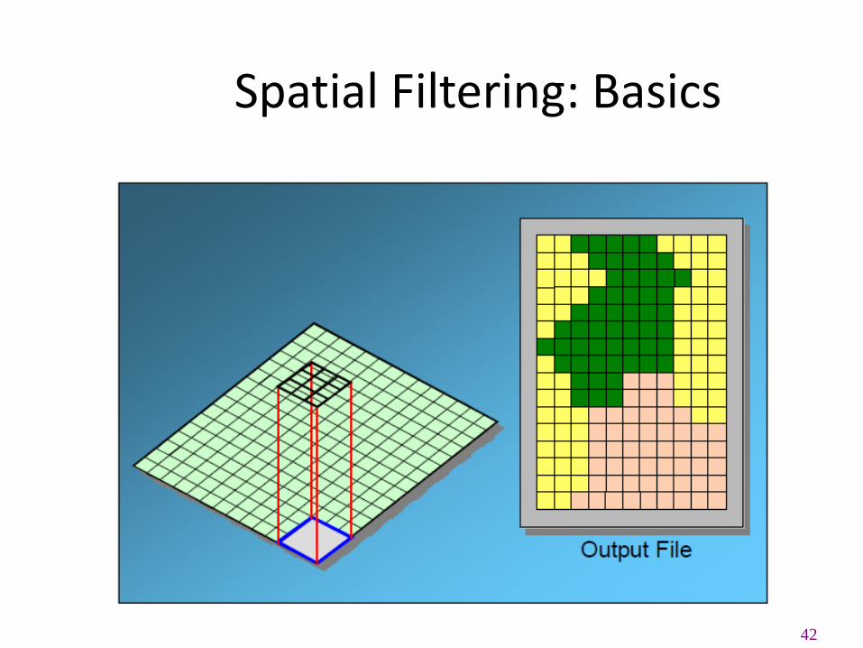
Moving window (kernel)
scans the 3x3
neighborhood of every
pixel in the image
Original Image
38
Spatial Filtering: Basics
39
Spatial Filtering: Basics
40
Spatial Filtering: Basics
41
Spatial Filtering: Basics
42
Spatial Filtering: Basics
43
Spatial Filtering: Basics
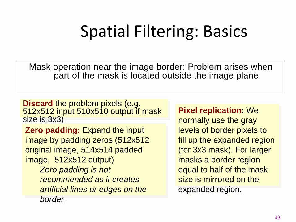
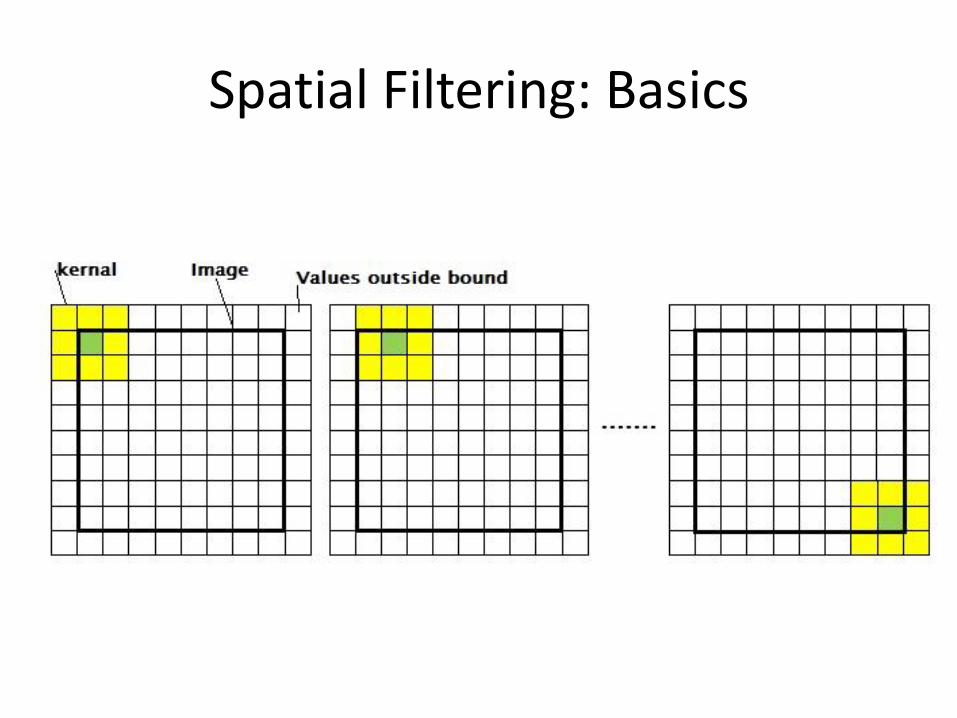
Mask operation near the image border: Problem arises when part of the mask is located outside the image plane
Discard the problem pixels (e.g. 512x512 input 510x510 output if mask size is 3x3)
Zero padding: Expand the input
image by padding zeros (512x512
original image, 514x514 padded
image, 512x512 output)
Zero padding is not
recommended as it creates
artificial lines or edges on the
border
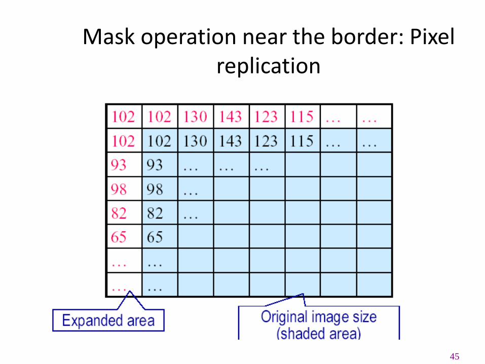
Pixel replication: We
normally use the gray
levels of border pixels to
fill up the expanded region
(for 3x3 mask). For larger
masks a border region
equal to half of the mask
size is mirrored on the
expanded region.
Spatial Filtering: Basics
45
Mask operation near the border: Pixel replication
46
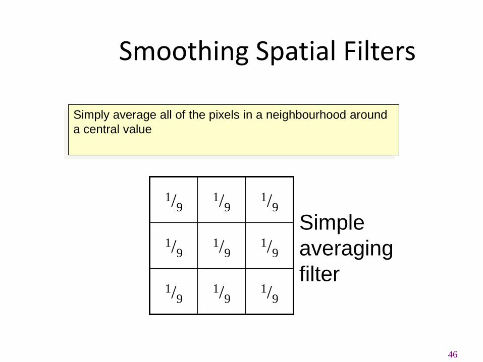
Smoothing Spatial Filters
Simply average all of the pixels in a neighbourhood around
a central value
1/9 1/9
1/9
1/9 1/9
1/9
1/9 1/9
1/9
Simple
averaging
filter
47
Smoothing Spatial Filters
For blurring/noise reduction
Blurring is usually used in preprocessing steps, e.g., to remove
small details from an image prior to object extraction, or to bridge
small gaps in lines or curves
Equivalent to Low-pass spatial filtering in frequency domain
because smaller (high frequency) details are removed based on
neighborhood averaging (averaging filters)
48
Smoothing Spatial Filters
1/9 1/9
1/9
1/9 1/9
1/9
1/9 1/9
1/9
Origin x
y Image f (x, y)
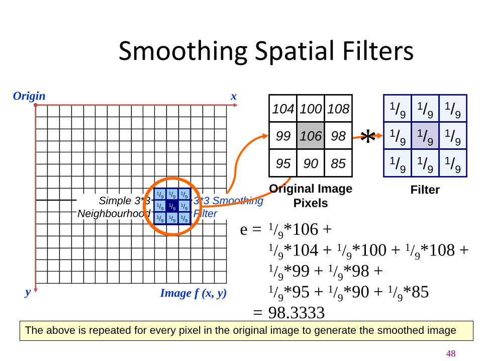
e = 1/9*106 +
1/9*104 + 1/9*100 + 1/9*108 +
1/9*99 + 1/9*98 +
1/9*95 + 1/9*90 + 1/9*85
= 98.3333
Filter Simple 3*3
Neighbourhood 106
104
99
95
100 108
98
90 85
1/9 1/9
1/9
1/9 1/9
1/9
1/9 1/9
1/9
3*3 Smoothing
Filter
104 100 108
99 106 98
95 90 85
Original Image
Pixels
*
The above is repeated for every pixel in the original image to generate the smoothed image
49
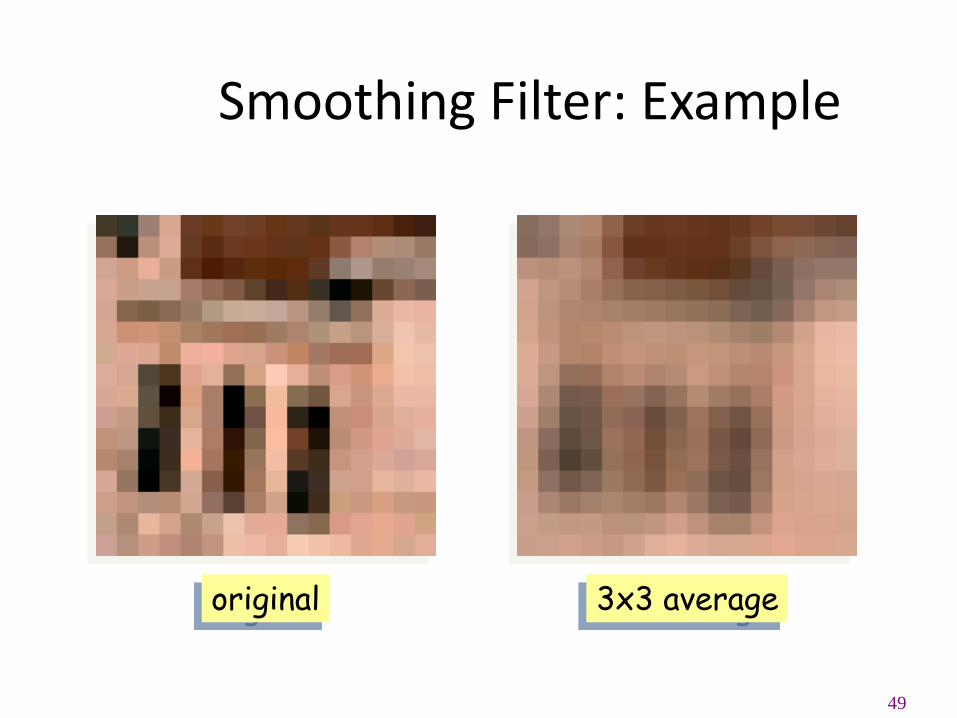
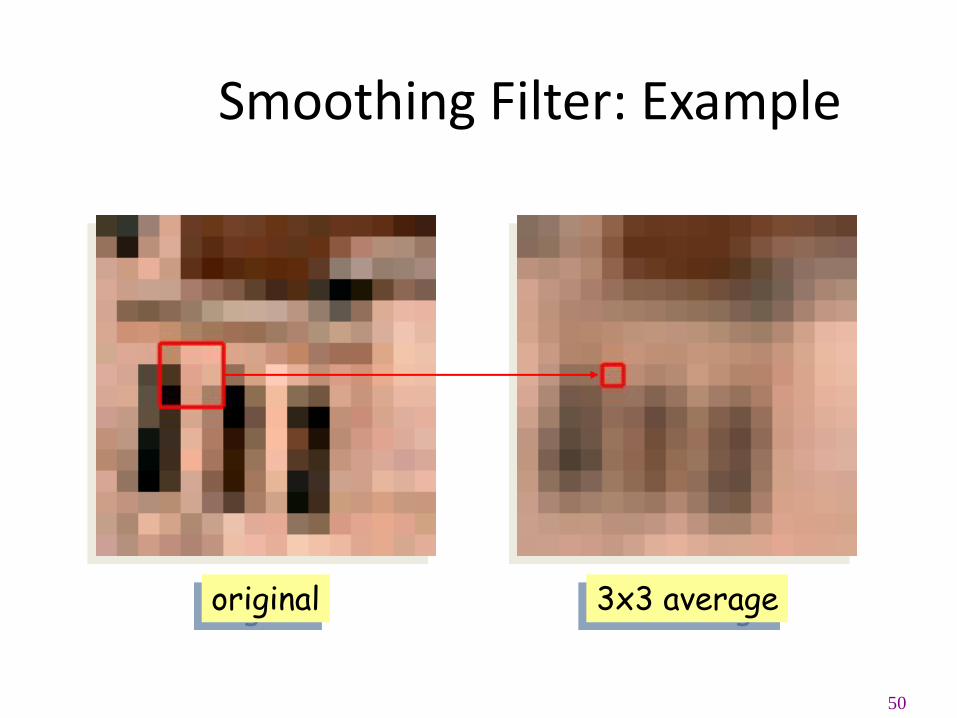
Smoothing Filter: Example
original 3x3 average
50
Smoothing Filter: Example
original 3x3 average

51
Smoothing Filter: Example
original 3x3 average
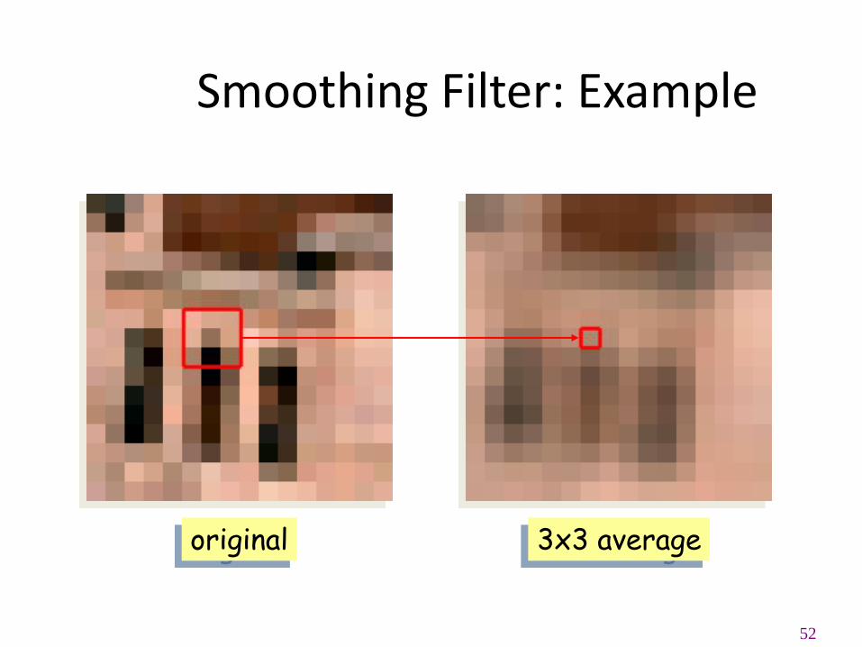
52
Smoothing Filter: Example
original 3x3 average
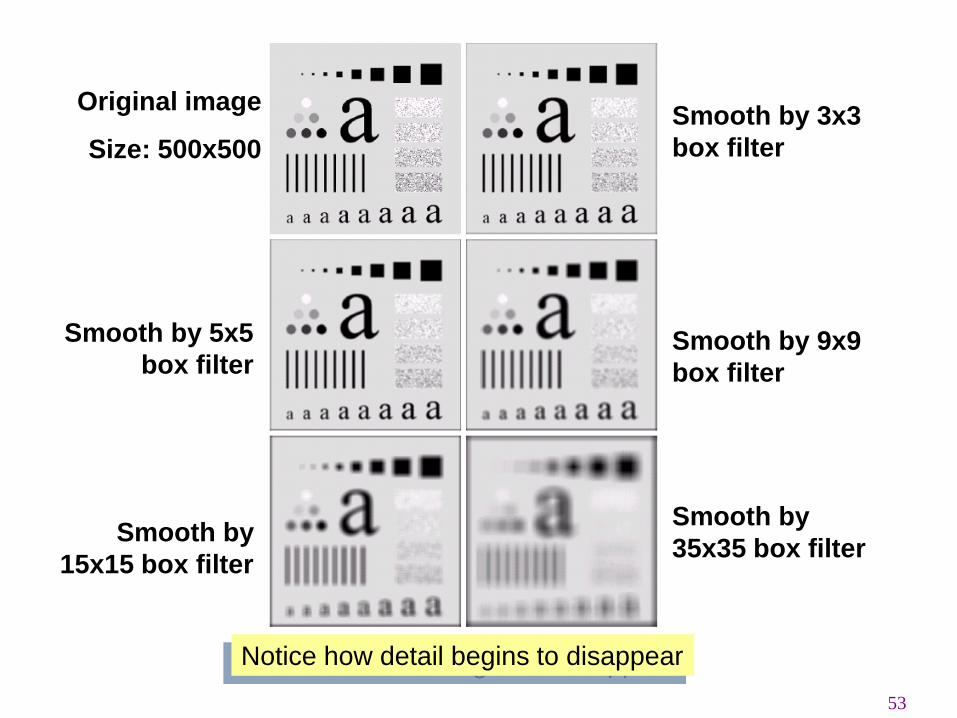
53
Original image
Size: 500x500
Smooth by 3x3
box filter
Smooth by 5x5
box filter Smooth by 9x9
box filter
Smooth by
15x15 box filter
Smooth by
35x35 box filter
Notice how detail begins to disappear
54
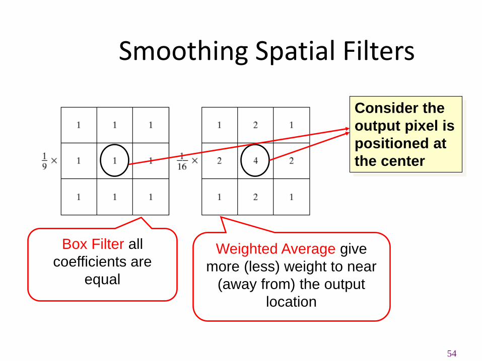
Smoothing Spatial Filters
Box Filter all
coefficients are
equal
Weighted Average give
more (less) weight to near
(away from) the output
location
Consider the
output pixel is
positioned at
the center
Readings from Book (3rd Edn.)
• 3.3 Histogram
• 3.5 Spatial filtering
56
Acknowledgements
Digital Image Processing”, Rafael C. Gonzalez & Richard E. Woods, Addison-Wesley,
2002
Peters, Richard Alan, II, Lectures on Image Processing, Vanderbilt University, Nashville,
TN, April 2008
Brian Mac Namee, Digitial Image Processing, School of Computing, Dublin Institute of
Technology
Computer Vision for Computer Graphics, Mark Borg
Ma
teria
l in
th
ese
slid
es h
as b
ee
n ta
ke
n fro
m, th
e f
ollo
win
g r
esou
rces