Lecture 4: Urban Amenities - princeton.eduerossi/Urban/Lecture_4_538.pdf · Introduction Role of...
25
Lecture 4: Urban Amenities WWS 582a Esteban Rossi-Hansberg Princeton University ERH (Princeton University ) Lecture 4: Urban Amenities 1 / 25
Transcript of Lecture 4: Urban Amenities - princeton.eduerossi/Urban/Lecture_4_538.pdf · Introduction Role of...

Lecture 4: Urban AmenitiesWWS 582a
Esteban Rossi-Hansberg
Princeton University
ERH (Princeton University ) Lecture 4: Urban Amenities 1 / 25

Introduction
Role of urban density in facilitating consumption has been found to beimportant: agglomeration force
Other urban amenities are important as well: like weather, shores, lakes,rivers, etc.
In the literature these forces have in general played a secondary role
However, the evidence seems to suggest that they are becoming moreimportant over time
I Modern city based on amenities?I Role of ICT?
Glaeser, Kolko, and Saiz (2001) is one of the first papers to document thisempirically in a robust way
ERH (Princeton University ) Lecture 4: Urban Amenities 2 / 25

Glaeser, Kolko, and Saiz (2001)
Four critical urban amenities:
1 Presence of a variety of services and consumer goods
1 Cities with more restaurants and theaters have grown faster2 In cities with more educated populations rent growth is faster than wagegrowth since 1970
2 Aesthetics and Physical Characteristics
1 Weather is the main determinant of population or housing price growth
3 Public Services
1 More crime leads to less urban growth
4 Speed
1 Higher value of time leads to higher rents in areas with easy access
ERH (Princeton University ) Lecture 4: Urban Amenities 3 / 25

Stylized facts: Reverse Commuting
TABLE 1Commuting patterns - US Metropolitan Areas
Daily Commutes (millions) Annualized growth rate
City-city 18.8 20.9 24.3 0.52% 1.52%City-suburb 2.0 4.2 5.9 3.65% 3.46%City-other 0.6 1.2 1.9 3.63% 4.70%Suburb-city 6.6 12.7 15.2 3.34% 1.81%Suburb-suburb 11.3 25.3 35.4 4.09% 3.42%Suburb-other 1.1 3.7 6.8 6.22% 6.27%
Total 40.5 68.0 89.5 2.62% 2.79%
Sowce : Commuting in America. EN0 Transportation Foundation
ERH (Princeton University ) Lecture 4: Urban Amenities 4 / 25

Stylized facts: Reverse Commuting
TABLE 2Reverse commuting in the San Francisco Bay Area Counties
% change of % change of employeesemployment in county living in county
(1) (4 W(1)
San FranciscoSan MateoSanta ClaraAlamedaContra CostaSolanoNapaSonomaMarin
9.2%22.0%25.1%21.5%47.1%35.5%33.6%51.0%24.7%
14.5%14.0%22.1%24.7%33.7%57.0%24.9%51.0%8.7%
5.3%-7.9%-3.0%3.1%
-13.5%21.5%-8.7%0.0%
-16.0%
Source : Census Tabulations from the Metropolitan Transportation Comission, San Francisco Bay Area
ERH (Princeton University ) Lecture 4: Urban Amenities 5 / 25

Stylized facts: The Success of High Amenity CitiesTABLE 3
Population growth and amenities
Pouulation Growth
UNITED STATES (77-95) Estimate t-value
Temperate climate 0.35 17.8Proximity to ocean coast 0.24 12.5Live performance venues per capita 0.14 6Dry climate 0.12 6.5Restaurants per capita 0.05 2.9Art museums per capita -0.03 -1.5Movie theaters per capita -0.05 -2.6Bowling alleys per capita -0.19 -11.3
FRANCE (1975-1990)
Restaurants per capitaHotel rooms per capita
0.45 50.33 4
ENGLAND (1981-1997)
Tourist nights per capita 0.31 2.7
Notes : Each coeffkient is the result of a separate regression of population growthon each amenity and other controls. The values of the variables were transformedto have standard error=1 .The temperate climate variable is the inverse of (averagetemperature per year-70 degrees). All temperatures are measured in Farenheitdegrees. Dry climate stands for the inverse of average precipitation. US regressionsincluded controls for county density, share of college educated, and a shift-shareindustry growth measure. France observation units are the “Zones d’Emploi”.France regressions included controls for participation rate and population in 1975.The England regression is for counties, as defined in the Data Appendix. TheEngland regression included a dummy for Northern counties and initial populationas controls.
ERH (Princeton University ) Lecture 4: Urban Amenities 6 / 25

Stylized facts: The Success of High Amenity Cities
TABLE 4
Ranking of Top and Bottom US MSA’s, according toEstimated Amenity Value
Metropolitan Statzstrcal Area (MSAI.
Highest Lowest
Honolulu, HISanta Cruz, CASanta Barbara-Santa Maria-Lompoc, CASalinas-Seaside-Monterey, CALos Angeles-Long Beach, CASan Francisco, CASan Jose, CASanta Rosa-Petaluma, CAOxnard-Ventura, CASan Diego, CA
Stamford, CTNorwalk, CTAnchorage, AKRochester, MNDetroit, MIMidland, TXTrenton, NJMinneapolis-St.Paul, MNNassau-Suffolk, NYBloomington-Normal, IL
Notes : Estimated Amenity Value measured as residual from an OLS regression of log medianhouse value on log median income in 1990.
ERH (Princeton University ) Lecture 4: Urban Amenities 7 / 25
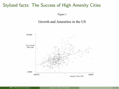
Stylized facts: The Success of High Amenity Cities
Figure 1
Growth and Amenities in the US
-.481973 .66906
-.15964
.507808
Pop. Growth 1980-1990
Amenity Value 1980
ERH (Princeton University ) Lecture 4: Urban Amenities 8 / 25

Stylized facts: The Demand for Urban Amenities is Rising
TABLE 5
Correlation between estimated amenity valueand population
Amenity-Population correlation
us 1980 0.221990 0.36
ERH (Princeton University ) Lecture 4: Urban Amenities 9 / 25

Stylized facts: The Demand for Urban Amenities is Rising
TABLE 6
Elasticities with respect to population size
U S 19801990
wages housing prices
0.05 1 0.1140.082 0.225
wages housing rents
England 1988 0.047 0.0361998 0.072 0.021
Notes: Population at the MSA level for US, county level for England. See DataAppendix for data description.
ERH (Princeton University ) Lecture 4: Urban Amenities 10 / 25

Stylized facts: The Demand for Urban Amenities is Rising
TABLE 7Wage and rent growth in Paris and London
ENGLAND (1988- 1998)
LondonRest of England
Difference-in-difference(London amenity premium)
Wage growth
4.90%4.70%
Rent growth
8.60%7.50%
0.90%
FRANCE (1990-1995)
Parisrest of France
difference-in-difference(Paris amenity premium)
3.60% 4.20%4.00% 3.50%
1.10%
Notes : Annualized growth rates. See Data Appendix for data sources
ERH (Princeton University ) Lecture 4: Urban Amenities 11 / 25

Stylized facts: The Demand for Urban Amenities is Rising
TABLE 8
Income and housing value growth in selected American cities
1993-1998
Income growth Home value growth Difference
San FranciscoBostonChicagoNew York CityLos AngelesWashington, DC
2.46% 4.51% 2.05%3.11% 4.65% 1.54%3.64% 3.76% 0.12%2.69% 2.57% -0.12%1.82% 1.21% -0.61%3.83% 1.12% -2.71%
Notes: Annual growth rates over the 1993-1998 period
ERH (Princeton University ) Lecture 4: Urban Amenities 12 / 25

Stylized facts: Increasing Wealth of the Inner CityTABLE 9
Population distribution within the city
Panel A: All MSAs
Share of City Population Living: 1980 1990
Within one mile of CBDOne to three miles of CBDThree to five miles of CBDBeyond five miles of CBD
10.70% 10.30%35.50% 34.00%21.90% 21.80%31.90% 33.90%
Panel B: 10 biecest MSAs.
Share of City Population Living:
Within one mile of CBDOne to three miles of CBDThree to five miles of CBDBeyond five miles of CBD
1980 1990
4.80% 4.90%17.00% 16.50%19.00% 18.40%59.20% 60.20%
Notes : See data Appendix for data sources.
ERH (Princeton University ) Lecture 4: Urban Amenities 13 / 25

Stylized facts: Increasing Wealth of the Inner City
TABLE 10Income distribution within the city
Panel A: All MSAs
Income Relative to Citv AveraPe 1980 1990
Within one mile of CBDOne to three miles of CBDThree to five miles of CBDBeyond five miles of CBD
89% 94%95% 95%101% 100%109% 107%
Panel B: 10 biggest MSAs
Income Relative to Citv Averape 1980 1990
Within one mile of CBDOne to three miles of CBDThree to five miles of CBDBeyond five miles of CBD
144% 163%88% 97%86% 86%105% 100%
Notes : See data Appendix for data sources.
ERH (Princeton University ) Lecture 4: Urban Amenities 14 / 25

Stylized facts: Increasing Wealth of the Inner City
Manhattan: median income by tract, 1990
F i g u r e 2
.0 - 85778578 - 2500625007 - 3639236393 - 5431754318 - 7605076051 - 100098100099 - 132171132172 - 174487174488 - 238502238503 - 327320
N
EW
S
Manhattan: median income by tract 1990
ERH (Princeton University ) Lecture 4: Urban Amenities 15 / 25
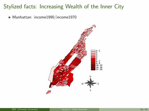
Stylized facts: Increasing Wealth of the Inner City
Manhattan: income1990/income1970
Figure 3
Manhattan: income 1990/income 1970
.0 - 123456 - 78 - 910 - 1314 - 1617 - 25
N
EW
S
ERH (Princeton University ) Lecture 4: Urban Amenities 16 / 25

Stylized facts: Increasing Wealth of the Inner City
Manhattan: median rent 1990/median rent 1980
Figure 4
Manhattan: median rent 90/ median rent 80
.0 - 0.6520.652 - 1.6871.687 - 1.9131.913 - 2.0652.065 - 2.2272.227 - 2.4422.442 - 2.7362.736 - 3.343.34 - 4.0494.049 - 5.952
N
EW
S
ERH (Princeton University ) Lecture 4: Urban Amenities 17 / 25

Estmating Productivity and Amenities for US Counties
Can identify a topography of productivities A and amenities u consistent withestimates transport costs and observed distribution of economic activity(wages, w , and population, L)
I Use model in Allen and Arkolakis (2014)
Intuition: consider locations i and j with identical bilateral trade costs.Thensince u = w (i )
P (i ) a(i)
I Utility equalization implies a(i )a(j) =w (j)/P (j)w (i )/P (i ) .
I Balanced trade identifies A(i )A(j)
Note: A and u cannot be identified without knowledge of externalityelasticity (α for production, β for amenities)
ERH (Princeton University ) Lecture 4: Urban Amenities 18 / 25

Observed LEstimating A and u: Observed L
ERH (Princeton University ) Lecture 4: Urban Amenities 19 / 25

Observed wEstimating A and u: Observed w
ERH (Princeton University ) Lecture 4: Urban Amenities 20 / 25

Productivity
α = 0.1Estimating A and u: Exogenous A (α = 0.1)
ERH (Princeton University ) Lecture 4: Urban Amenities 21 / 25

Amenitiesβ = −0.3Estimating A and u: Exogenous u (β = −0.3)
ERH (Princeton University ) Lecture 4: Urban Amenities 22 / 25

Moving to Nice Weather (Rappaport, 2007)
you move to the lower right. The underlying loss function assumes 75°F to be the year-roundideal.2
The introduction of air conditioning lessens the disutility from hot summer weather.Individuals become willing to endure more of it in return for warm winter weather. Equivalently,the indifference curves stretch rightward along the top vertical axis. This causes numerouspreference reversals. For example, Duluth Minnesota's weather without air conditioning ispreferred to that of numerous cities in the South and Southwest. But with AC, Duluth's weather isthe least preferred among the depicted cities. Similarly, numerous cities in the bottom left of thefigure reverse from having relatively desirable to relatively undesirable weather.
Restoring spatial equilibrium requires a new vector of wages and house prices across places. Ingeneral, themore the valuation of a place's weather has risen, the larger the required fall in its relativewage and increase in its relative house price. Migration brings about the new spatial equilibrium.People will move both towards places with hot summers and places with warm winters (that is,towards the upper right of the figure). The impulse towards hot summers is intuitive: hot weather hasbecome “less bad”. The impulse towards warmwinters arises because AC increases the sensitivity ofrelativeweather valuations towinter temperatures. This is reflected in the flatter indifference curves.3
2 Specifically, the loss function is assumed to be of the form, L=a|s− s⁎|~+b|w−w⁎|β. Here s and w are respectivelysummer and winter temperature. The remaining elements of the equation are positive parameters. The introduction of ACis depicted as a decrease in a. Improved heating might correspond to a decrease in b. An increased valuation of niceweather might correspond to increases in both a and b.3 An illustrative example, in the upper middle of Fig. 1, is the required faster relative growth of Riverside compared to
Bakersfield, notwithstanding that the two cities' summer weather is virtually identical. Prior to AC, the two cities'weather bundles were equally valued. With AC, Riverside's weather is preferred to that of Bakersfield.
Fig. 1. Iso-utility over weather.
379J. Rappaport / Regional Science and Urban Economics 37 (2007) 375–398
ERH (Princeton University ) Lecture 4: Urban Amenities 23 / 25

Moving to Nice Weather
larger as temperatures increase. This increasing quadratic relationship is intuitive if the advantageof warmer winter weather is the chance to participate in many outdoor recreational activities. BothJuly heat index and July relative humidity have negative, statistically significant coefficients ontheir linear terms. Expected population growth falls as summer heat index and relative humidityincrease from their respective sample means of 98°F and 66%.8
8 The negative partial correlation of population growth with summer temperature holds only when controlling forwinter temperature. Otherwise, a positive coefficient on July heat index statistically differs from zero at the 0.05 level.This statistically-significant positive partial correlation of growth with summer temperature in the absence of a control forwinter temperature is quite robust across alternative specifications.
Table 3Population growth and weather
(1) (2) (3) (4) (5) (6)
Dependent variable →Independent variables ↓
Annual population growth rate, 1970 to 2000
Coast/river/topography (7) No Yes Yes Yes Yes YesInitial density spline (7) No No Yes Yes Yes YesConcentric total pop (7) No No Yes Yes Yes YesAg/mnrl/mnfct (17) No No No Yes Yes YesCensus divisions (8) No No No No Yes NoWeighted regression No No No No No yes
January daily max temp Linear 0.0751 0.0663 0.0655 0.0513 0.0497 0.0488(0.0098) (0.0104) (0.0099) (0.0093) (0.0099) (0.0092)
Quadratic 0.0012 0.0012 0.0014 0.0013 0.0016 0.0013(0.0004) (0.0004) (0.0004) (0.0003) (0.0003) (0.0003)
July daily heat index Linear −0.0626 −0.0508 −0.0505 −0.0215 −0.0242 −0.0170(0.0116) (0.0127) (0.0126) (0.0112) (0.0114) (0.0114)
Quadratic −0.0002 −0.0003 0.0004 −0.0006 −0.0002 −0.0008(0.0005) (0.0005) (0.0005) (0.0005) (0.0005) (0.0005)
July daily rel humidity Linear −0.0371 −0.0410 −0.0621 −0.0395 −0.0549 −0.0385(0.0142) (0.0147) (0.0162) (0.0129) (0.0132) (0.0123)
Quadratic 0.0005 0.0006 −0.0001 −0.0003 −0.0008 −0.0003(0.0005) (0.0005) (0.0004) (0.0004) (0.0003) (0.0004)
Annual precipitation Linear 0.0216 0.0231 0.0153 −0.0044 −0.0029 −0.0048(0.0107) (0.0107) (0.0100) (0.0082) (0.0087) (0.0080)
Quadratic −0.0004 −0.0004 0.0001 0.0002 0.0002 0.0002(0.0002) (0.0002) (0.0002) (0.0001) (0.0001) (0.0001)
Annual precipitation days Linear 0.0053 0.0041 0.0021 0.0064 0.0061 0.0065(0.0060) (0.0060) (0.0061) (0.0048) (0.0054) (0.0047)
Quadratic −0.0002 −0.0002 −0.0003 −0.0002 −0.0002 −0.0002(0.0001) (0.0001) (0.0001) (0.0001) (0.0000) (0.0001)
Observations 3067 3067 3067 3067 3067 3067# of indep. variables 10 17 31 48 56 48R-squared 0.272 0.282 0.382 0.503 0.517 0.497Control variables R-squared 0.094 0.226 0.433 0.471 0.423Marginal R-squared 0.188 0.156 0.070 0.046 0.074
Table shows results from regressing ([log(2000 Pop Density)− log(1970 Pop Density)]×100/30) on the enumerated weathervariables, control variables, and a constant. Quadratic weather variables have had their respective sample mean subtracted.Standard errors in parentheses are robust to a spatial correlation using the procedure discussed in the main text. Bold typesignifies coefficients that statistically differ from zero at the 0.05 level. Italic type signifies coefficients that statistically differentfrom zero at the 0.10 level. The Column 6 regression weights observations according to 1/ (1+3000/population).
387J. Rappaport / Regional Science and Urban Economics 37 (2007) 375–398
ERH (Princeton University ) Lecture 4: Urban Amenities 24 / 25

Moving to Nice Weather
expected population growth is 1.3 percentage points slower than that of a county with meanannual precipitation days.
The five weather variables in Table 3 – each entered linearly and quadratically – account for avery large share of the variance of population growth. The R-squared value from the regressionwith no controls is 0.272. For comparison, a regression of population growth on forty-eightcontinental U.S. state dummies yields an R-squared value of 0.322. Additionally including theweather variables with the controls in the baseline Column 4 regression increases R-squared by7.0 percentage points. Again for comparison, the marginal R-squared value from adding statedummies to the baseline controls is 12.4 percentage points.
Fig. 2 shows the expected population growth attributable to weather as estimated by thebaseline regression.13 In other words, it shows the vector product of the ten coefficients reportedin Column 4 with counties' actual linear and quadratic weather values. The resulting expectedgrowth captures the marginal effect of weather after controlling for coastal proximity, topography,initial density, initial surrounding population, and initial industrial composition. Expected growthfrom the weather is highest in southern Florida, southwestern Texas, southern New Mexico,southern Arizona, southern California, and coastal northern California. Expected growth from theweather is lowest throughout most of New England and the Midwest as well as in West Virginiaand the Pacific Northwest.
The faster expected growth of places with cooler and less humid summers establishes that airconditioning cannot alone account for the move to nice weather. This point is nicely illustrated inFig. 2 by the high expected growth of California's coastal counties. These counties' mild summerweather implies that their rapid growth cannot be attributed to air conditioning. Conversely, if airconditioning were the main force driving weather-related moves, then expected growth would bemuch higher throughout the Deep South (one of the hottest and most humid areas of the U.S.).
Fig. 2. Expected population growth from weather (1970 to 2000). Figure shows the fitted annual population growth ratecontrolling for coast, topography, initial density, concentric population, and industrial composition.
13 A color version is included in the paper's supplemental materials.
390 J. Rappaport / Regional Science and Urban Economics 37 (2007) 375–398
ERH (Princeton University ) Lecture 4: Urban Amenities 25 / 25