Lecture 4 Scattering theory - University of...

1

Lecture 4Lecture 4Scattering theoryScattering theory

SS2011SS2011: : ‚‚Introduction to Nuclear and Particle Physics, Part 2Introduction to Nuclear and Particle Physics, Part 2‘‘

2

I. Scattering experimentsI. Scattering experiments

Scattering experiment:

A beam of incident scatterers with a given flux or intensity (number of particles per unit area dA per unit time dt ) impinges on the target (described by a scattering potential);

the flux can be written as

The number of particles per unit time which are detected in a small region of the solid angle, dΩ, located at a given angular deflection specified by (θ, φ), can be counted as

3

Scattering cross sectionScattering cross sectionThe differential cross-section for scattering is defined as the number of particles scattered into an element of solid angle dΩ in the direction (θ,φ) per unit time :

The total cross-section corresponds to scatterings through any scattering angle:

[dimensions of an area]

(1.2)

(1.1)ΩΩ

φϑσd

dNJ

1d

),(d sc

inc

=

Most scattering experiments are carried out in the laboratory (Lab) frame in which thetarget is initially at rest while the projectiles are moving. Calculations of the cross sectionsare generally easier to perform within the center-of-mass (CM) frame in which the centerof mass of the projectiles–target system is at rest (before and after collision)

one has to know how to transform the cross sections from one frame into the other.

Note: the total cross section σ is the same in both frames, since the total number of collisions that take place does not depend on the frame in which the observation is carriedout. However, the differential cross sections dσ/dΩ are not the same in both frames, since the scattering angles (θ,φ) are frame dependent.

Jinc - incident flux

4

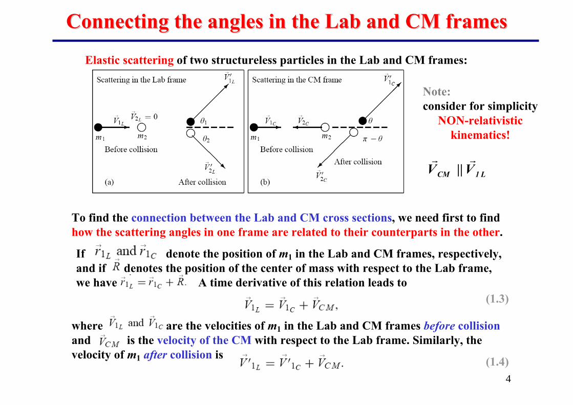
Connecting the Connecting the aanglesngles in the Lab and CM framesin the Lab and CM frames

To find the connection between the Lab and CM cross sections, we need first to find how the scattering angles in one frame are related to their counterparts in the other.

If denote the position of m1 in the Lab and CM frames, respectively, and if denotes the position of the center of mass with respect to the Lab frame,we have A time derivative of this relation leads to

where are the velocities of m1 in the Lab and CM frames before collisionand is the velocity of the CM with respect to the Lab frame. Similarly, the velocity of m1 after collision is

(1.3)

(1.4)

Elastic scattering of two structureless particles in the Lab and CM frames:

Note: consider for simplicity

NON-relativistic kinematics!

L1CM V||Vrr

5


(1.5)

(1.6)

Dividing (1.6) by (1.5), we end up with

(1.7)

(1.8)

(1.9)

Since from (1.8)

or from (1.9)

L22L11CM21

L2L1CM

VmVmV)mm(

ppprrr

rrr

+=+

+=Use that CM momenta

(1.10)

(1.11)

L1CM V||Vrr

Since

6


Since the center of mass is at rest in the CM frame, the total momenta before and after collisions are separately zero:

(1.12)

(1.13)

(1.14)

Since the kinetic energy is conserved:

(1.15)

(1.16)

In the case of elastic collisions, the speeds of the particles in the CM frame are the same before and after the collision;

From (1.11)

(1.17)Dividing (1.9) by (1.16)

0pppppp C2C1CC2C1C =′+′=′=+=rrrvrr

7

Note: In a similar way we can establish a connection between θ2 and θ.

From (1.4) we have + using

the x and y components of this relation are

Finally, a substitution of (1.17) into (1.7) yields

and usingwe obtain


(1.17)

(1.18)

(1.19)

(1.20)

8

Connecting the Lab and CM Cross SectionsConnecting the Lab and CM Cross SectionsThe connection between the differential cross sections in the Lab and CM frames can be obtained from the fact that the number of scattered particles passing through an infinitesimal cross section is the same in both frames:

What differs is the solid angle dΩ :

in the Lab frame:

in the CM frame:

Since there is a cylindrical symmetry around the direction of the incident beam

From (1.18)

(1.21)

(1.22)

(1.23)

(1.24)

9

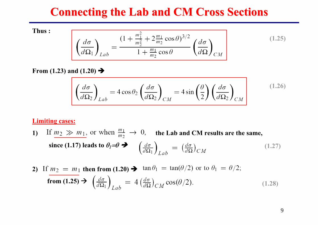
Limiting cases:

1) the Lab and CM results are the same,

since (1.17) leads to θ1=θ

2) then from (1.20)

from (1.25)

Connecting the Lab and CM Cross SectionsConnecting the Lab and CM Cross SectionsThus :

(1.25)

(1.26)

From (1.23) and (1.20)

(1.27)

(1.28)

10

From classical to quantum scattering theoryFrom classical to quantum scattering theory

1. Classical theory:

- scattering of hard ‚spheres‘

- individual well-defined trajectories

2. Quantum theory:

- scattering of wave pakeges wave–particle duality

- probabilistic origin of scattering process

11

II. Classical tII. Classical trajectoriesrajectories and and ccrossross--ssectionsections

Scattering trajectories, corresponding to different impact parameters, b give different scattering angles θ.

All of the particles in the beam in the hatched region of area dσ = 2π bdb are scattered into the angular region (θ, θ + dθ)

The equations of motion for incident particle:

+ initial conditions:defines the trajectory

since initial kinetic energy

For a particle obeying classical mechanics:

the trajectory for the unbound motion, corresponding to a scattering event, is deterministically predictable, given by the interaction potential and the initial conditions;

the path of any scatterer in the incident beam can be followed, and its angular deflection is determined as precisely as required

(2.2)

(2.1)

(2.3)

12

Classical tClassical trajectoriesrajectories and and ccrossross--ssectionsections

The number of particles scattered per unit time into the angular region (θ, θ+dθ) with any value of φ can be written as

The knowledge of b(θ), obtained directly from Newton’s laws or other methods, is then sufficient to calculate the scattering cross-section.

For the scattering from nontrivial central forces, the trajectory can be obtained from the equations of motion by using energy- and angular momentum- conservation methods

E.g., one can rewrite

in the form

L - angular momentum

(2.4)

(2.5)

(2.6)

13

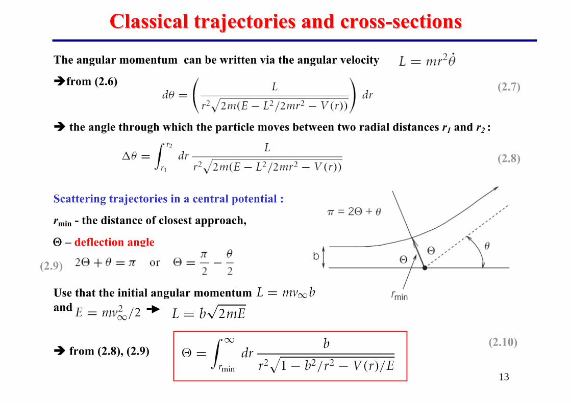
Classical tClassical trajectoriesrajectories and and ccrossross--ssectionsections

The angular momentum can be written via the angular velocity

from (2.6)

the angle through which the particle moves between two radial distances r1 and r2 :

Scattering trajectories in a central potential :

rmin - the distance of closest approach,

Θ – deflection angle

Use that the initial angular momentumand

(2.7)

(2.8)

(2.10)from (2.8), (2.9)

(2.9)

14

where the constant corresponds to the electrostatic interaction of point-like charges Z1e and Z2e

Classical Coulomb scatteringClassical Coulomb scattering

The potential corresponding to the scattering of charged particles via Coulomb’s law can bewritten in the general form

(2.11)

from (2.10)(2.12)

Note that for large energies (E→∞) or vanishing charges (A → 0), one has rmin → b

Use that

from (2.12)

(2.13)

(2.14)

15

Classical Coulomb scattering

Use that(2.15)

Rutherford formula - characteristic for Coulomb scattering from a point-like charge:

(2.16)

Note: If one attempts to evaluate the total cross-section using Eq. (2.16), one obtains aninfinite result. This divergence is due to the infinite range of the 1/r potential, and the “infinity” in the integral comes from scatterings as θ → 0 which corresponds to arbitrarily large impact parameters where the Coulomb potential causes a scatter through an arbitrarily small angle, which still contributes to the total cross-section.

16

III. Quantum ScatteringIII. Quantum ScatteringTheThe sscatteringcattering aamplitudemplitude of of sspinlesspinless,, nonrelativistic pnonrelativistic particlesarticles::

Consider the elastic scattering between two spinless, nonrelativistic particles of masses m1 and m2. During the scattering process, the particles interact with each other. If theinteraction is time independent, we can describe the two-particle system with stationary states (3.1)

(3.2)

where ET is the total energy and is a solution of the time-independent Schrödinger equation:

is the potential representing the interaction between the two particles.

In the case where the interaction between m1 and m2 depends only on their relative distance one can reduce the eigenvalue problem (3.2) to two decoupled eigenvalue problems:

one for the center of mass (CM), which moves like a free particle of mass M= m1+m2(which is of no concern to us here)

and another for a fictitious particle with a reduced mass which moves in the potential

(3.3)

17

Scattering of spinless particlesScattering of spinless particles

In quantum mechanics the incident particle is described by means of a wave packetthat interacts with the target.

After scattering, the wave function consists of an unscattered part propagating in theforward direction and a scattered part that propagates along some direction (θ,ϕ)

18


(3.3)

assume that V(r) has a finite range a: arif,0arif,0

)r(V̂>=≤≠

⎩⎨⎧

=

Outside the range, r > a, the potential vanishes, V(r)= 0; the eigenvalue problem (3.3) then becomes

(3.4)

One can consider (3.3) as representing the scattering of a particle of mass μ from a fixedscattering center described by V(r), where r is the distance from the particle μ to the centerof V(r):

In this case μ behaves as a free particle before the collision and can be described by a plane wave

where is the wave vector associated with the incident particle;A is a normalization factor.

Thus, prior to the interaction with the target, the particles of the incident beam are independent of each other; they move like free particles, each with a momentum

(3.5)

19

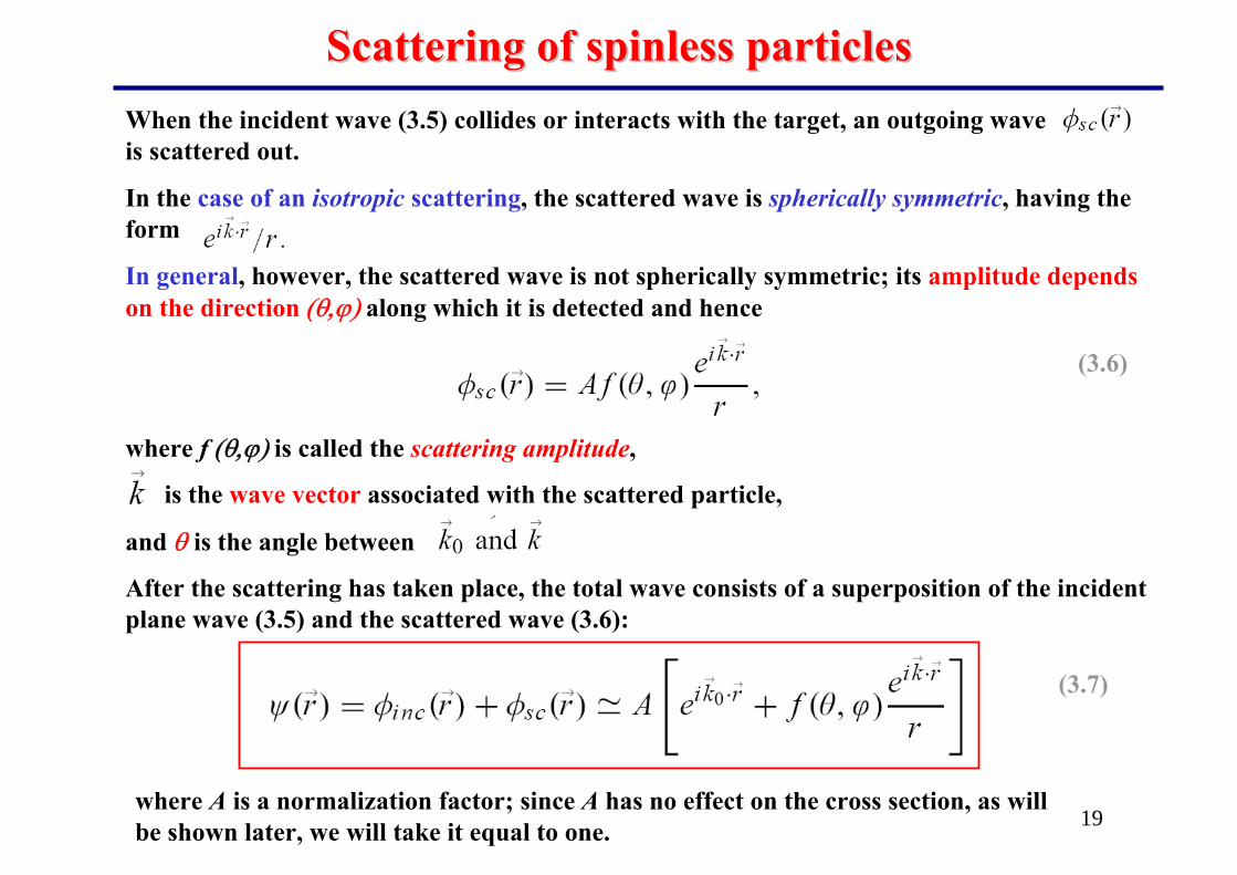
When the incident wave (3.5) collides or interacts with the target, an outgoing waveis scattered out.

In the case of an isotropic scattering, the scattered wave is spherically symmetric, having the form

In general, however, the scattered wave is not spherically symmetric; its amplitude depends on the direction (θ,ϕ) along which it is detected and hence

where f (θ,ϕ) is called the scattering amplitude,

is the wave vector associated with the scattered particle,

and θ is the angle between

After the scattering has taken place, the total wave consists of a superposition of the incidentplane wave (3.5) and the scattered wave (3.6):


(3.7)

(3.6)

where A is a normalization factor; since A has no effect on the cross section, as will be shown later, we will take it equal to one.

20

Scattering amplitude and differential cross sectionScattering amplitude and differential cross section

(3.9)

Introduce the incident and scattered flux densities:

(3.8)

Inserting (3.5) into (3.8) and (3.6) into (3.9) and taking the magnitudes of the expressionsthus obtained, we end up with

(3.10)

(3.11)

We recall that the number dN(θ,ϕ) of particles scattered into an element of solid angle dΩ in the direction (θ,ϕ) and passing through a surface element dA= r2dΩ per unit time is given as follows:

(3.12)Using (3.10)

21

Scattering amplitude and differential cross sectionScattering amplitude and differential cross section

(3.13)

By inserting (3.12) and in (1.1), we obtain:

Since the normalization factor A does not contribute to the differential cross section, itwill be taken to be equal to one.

For elastic scattering k0 is equal to k; so (3.13) reduces to

(3.14)

The problem of determining the differential cross section dσ/dΩ therefore reduces to that of obtaining the scattering amplitude f (θ,ϕ).

Lecture 4 Scattering theory - University of...

Documents

Transcript of Lecture 4 Scattering theory - University of...