Lecture 4 Data-Flow Scheduling Forrest Brewer. Data Flow Model Hierarchy Kahn Process Networks (KPN)...
94
Lecture 4 Lecture 4 Data-Flow Scheduling Data-Flow Scheduling Forrest Brewer
-
Upload
james-fleming -
Category
Documents
-
view
222 -
download
0
Transcript of Lecture 4 Data-Flow Scheduling Forrest Brewer. Data Flow Model Hierarchy Kahn Process Networks (KPN)...

Lecture 4Lecture 4Data-Flow SchedulingData-Flow Scheduling
Forrest Brewer

Data Flow Model HierarchyData Flow Model Hierarchy
Kahn Process Networks (KPN) (asynchronous task network) Dataflow Networks
– special case of KPN– actors, tokens and firings
Static Data Flow (Clocked Automata)– special case of DN– static scheduling– code generation– buffer sizing (resources!!)
Other Clocked Data Flow models– Boolean Data Flow– Dynamic Data Flow– Sequence Graphs, Dependency Graphs, Data Flow Graphs– Control Data Flow
Data Flow ModelsData Flow Models
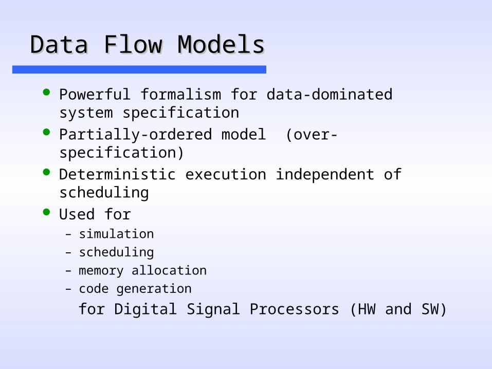
Powerful formalism for data-dominated system specification
Partially-ordered model (over-specification) Deterministic execution independent of scheduling Used for
– simulation– scheduling– memory allocation– code generation
for Digital Signal Processors (HW and SW)

Data Flow NetworksData Flow Networks
A Data Flow Network is a collection of actors which are connected and communicate over unbounded FIFO queues
Actors firing follows firing rules– Firing rule: number of required tokens on inputs
– Function: number of consumed and produced tokens Actors are functional i.e. have no internal state Breaking processes of KPNs down into smaller units of
computation makes implementation easier (scheduling) Tokens carry values
– integer, float, audio samples, image of pixels Network state: number of tokens in FIFOs
Intuitive semanticsIntuitive semantics
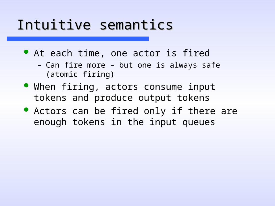
At each time, one actor is fired– Can fire more – but one is always safe (atomic firing)
When firing, actors consume input tokens and produce output tokens
Actors can be fired only if there are enough tokens in the input queues
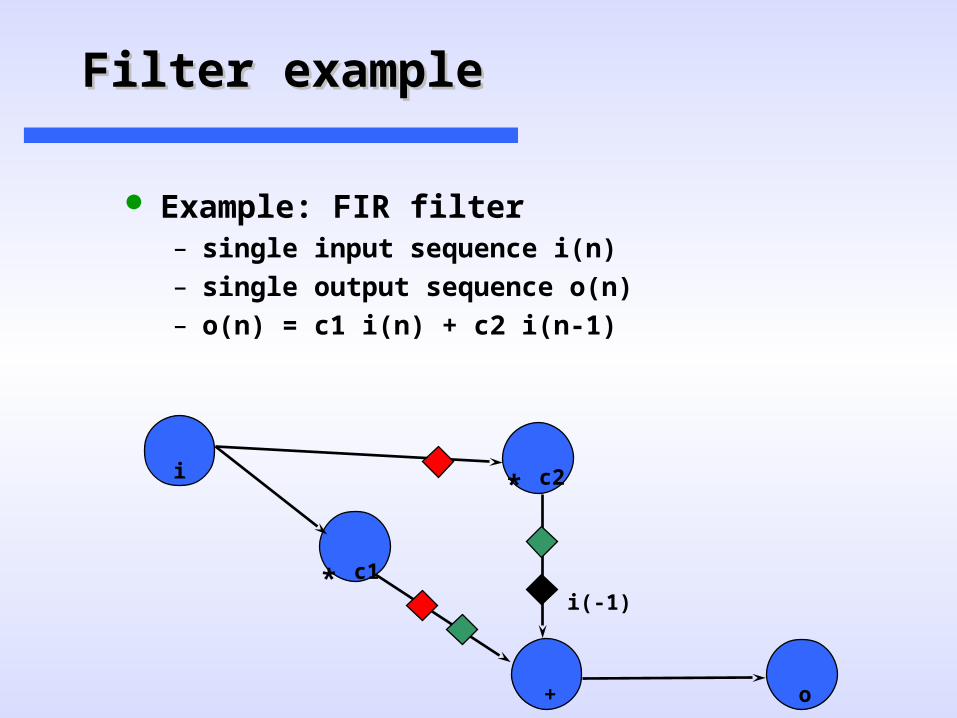
Filter exampleFilter example
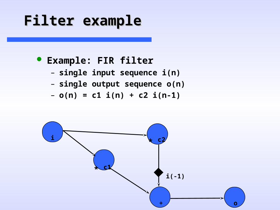
Example: FIR filter– single input sequence i(n)– single output sequence o(n)– o(n) = c1 i(n) + c2 i(n-1)
* c1
+ o
i * c2
i(-1)

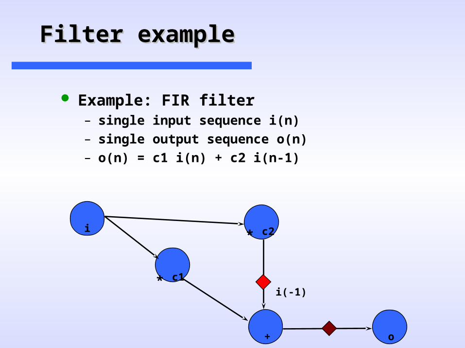
Filter exampleFilter example
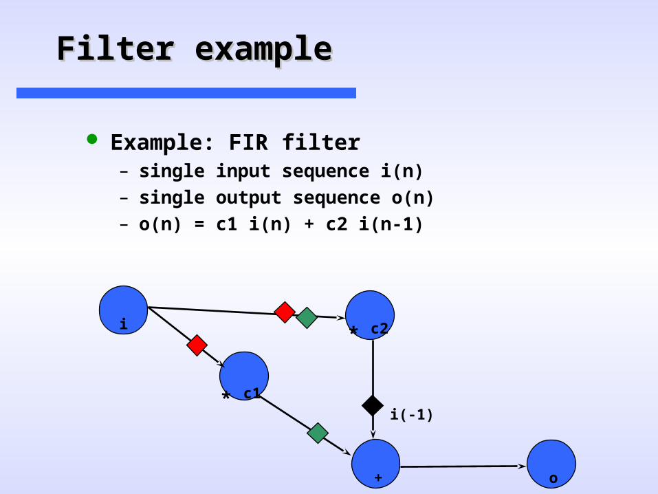
Example: FIR filter– single input sequence i(n)– single output sequence o(n)– o(n) = c1 i(n) + c2 i(n-1)
* c1
+ o
i * c2
i(-1)

Filter exampleFilter example
Example: FIR filter– single input sequence i(n)– single output sequence o(n)– o(n) = c1 i(n) + c2 i(n-1)
* c1
+ o
i * c2
i(-1)
Filter exampleFilter example
Example: FIR filter– single input sequence i(n)– single output sequence o(n)– o(n) = c1 i(n) + c2 i(n-1)
* c1
+ o
i * c2
i(-1)

Filter exampleFilter example
Example: FIR filter– single input sequence i(n)– single output sequence o(n)– o(n) = c1 i(n) + c2 i(n-1)
* c1
+ o
i * c2
i(-1)
Filter exampleFilter example
Example: FIR filter– single input sequence i(n)– single output sequence o(n)– o(n) = c1 i(n) + c2 i(n-1)
* c1
+ o
i * c2
i(-1)

Filter exampleFilter example
Example: FIR filter– single input sequence i(n)– single output sequence o(n)– o(n) = c1 i(n) + c2 i(n-1)
* c1
+ o
i * c2
i(-1)

Filter exampleFilter example
Example: FIR filter– single input sequence i(n)– single output sequence o(n)– o(n) = c1 i(n) + c2 i(n-1)
* c1
+ o
i * c2
i(-1)

Filter exampleFilter example
Example: FIR filter– single input sequence i(n)– single output sequence o(n)– o(n) = c1 i(n) + c2 i(n-1)
* c1
+ o
i * c2
i(-1)
Filter exampleFilter example
Example: FIR filter– single input sequence i(n)– single output sequence o(n)– o(n) = c1 i(n) + c2 i(n-1)
* c1
+ o
i * c2
i(-1)

Filter exampleFilter example
Example: FIR filter– single input sequence i(n)– single output sequence o(n)– o(n) = c1 i(n) + c2 i(n-1)
* c1
+ o
i * c2
i(-1)
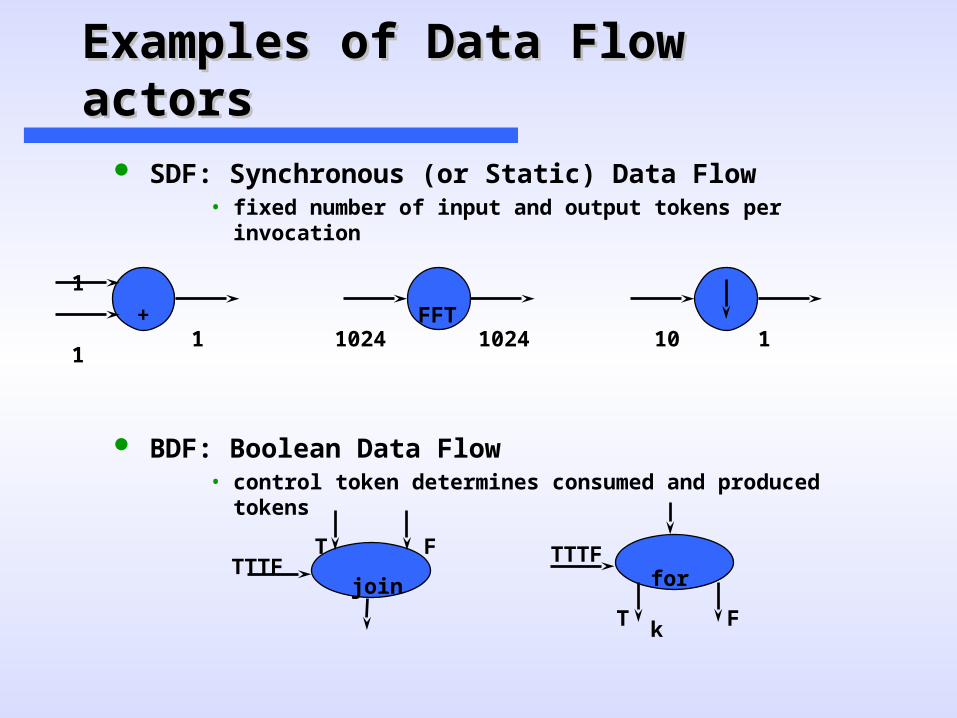
Examples of Data Flow actorsExamples of Data Flow actors
SDF: Synchronous (or Static) Data Flow• fixed number of input and output tokens per invocation
BDF: Boolean Data Flow• control token determines consumed and produced tokens
+
1
11
FFT1024 1024 10 1
join
T FTTTF for
k FT
TTTF

Examples of Data Flow actorsExamples of Data Flow actors
Sequence Graphs, Dependency Graph, Data Flow Graph
• Each edge corresponds to exactly one value• No buffering• Special Case of SDF
CDFG: Control Data Flow Graphs• Adds branching (conditionals) and iteration constructs• Many different models for this
+
1
11
+
1
1
+
1
1
Typical model in many behavioral/architectural synthesis toolsTypical model in many behavioral/architectural synthesis tools

Scheduling Data FlowScheduling Data Flow
Given a set of Actors and Dependencies How to construct valid execution sequences?
– Static Scheduling:Assume that you can predefine the execution sequence– FSM Scheduling:Sequencing defined as control-dependent FSM– Dynamic SchedulingSequencing determined dynamically (run-time) by predefined
rules In all cases, need to not violate resource or
dependency constraints In general, both actors and resources can
themselves have sequential (FSM) behaviors

(MIPS) RISC Instruction Execution (MIPS) RISC Instruction Execution
pc in
incr pc
fetch inst
inst out pc out
Operand Dependencies
inst in
read rs read rt
alu
write rd
Tasks

Another RISC Instruction ExecutionAnother RISC Instruction Execution
read rs
inst in
fetch inst
inst out
pc in
pc out
incr pc
write rd
read rt
alu
instdecode
Operand Resolution
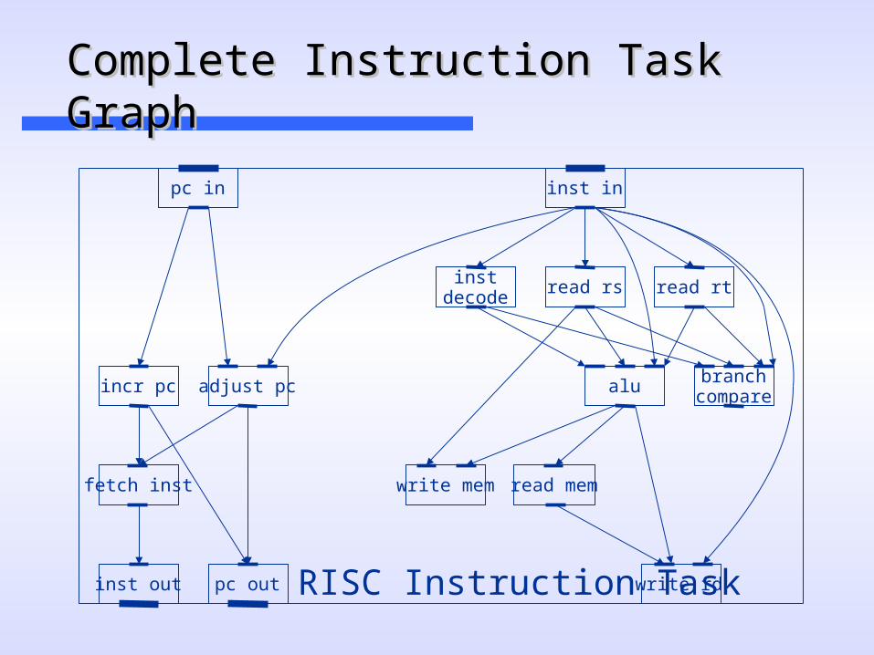
Complete Instruction Task GraphComplete Instruction Task Graph
read rs
inst in
fetch inst
inst out
pc in
pc out
incr pc
write rd
instdecode read rt
alu
read memwrite mem
adjust pc branchcompare
RISC Instruction Task
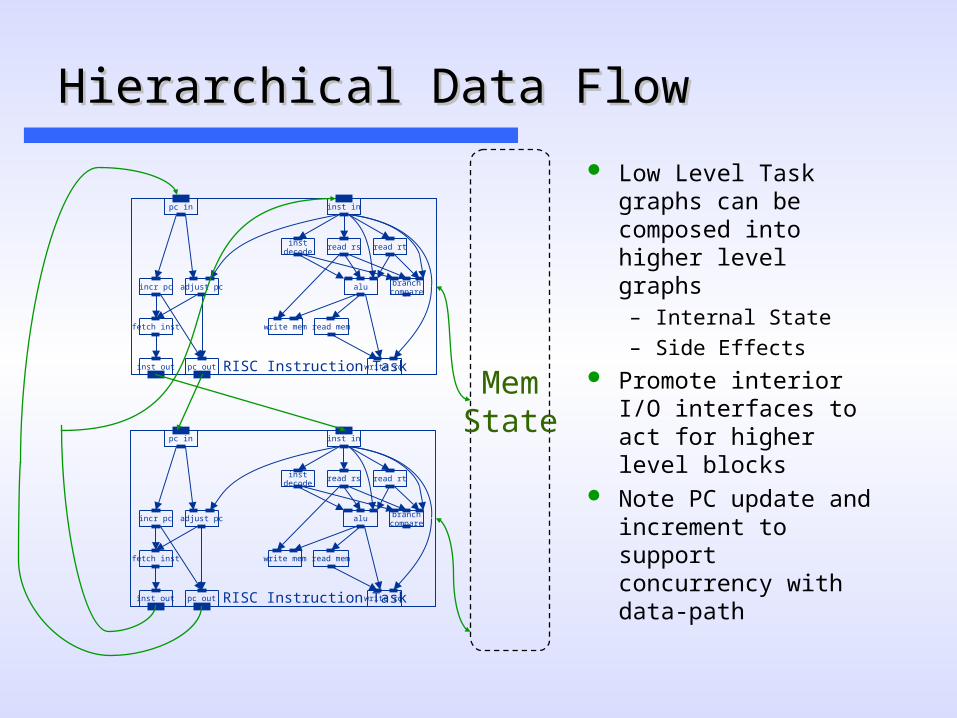
Hierarchical Data FlowHierarchical Data Flow
Low Level Task graphs can be composed into higher level graphs– Internal State
– Side Effects Promote interior I/O
interfaces to act for higher level blocks
Note PC update and increment to support concurrency with data-path
read rs
inst in
fetch inst
inst out
pc in
pc out
incr pc
write rd
instdecode
read rt
alu
read memwrite mem
adjust pc branchcompare
RISC Instruction Task
read rs
inst in
fetch inst
inst out
pc in
pc out
incr pc
write rd
instdecode
read rt
alu
read memwrite mem
adjust pc branchcompare
RISC Instruction Task
MemState

Scheduling Result: Valid SequencesScheduling Result: Valid Sequences
read rs
inst in
fetch inst
inst out
pc in
pc out
incr pc
write rd
instdecode read rt
alu
read memwrite mem
adjust pc branchcompare
RISC Instruction Task 0

read rs
inst in
fetch inst
inst out
pc in
pc out
incr pc
write rd
instdecode read rt
alu
read memwrite mem
adjust pc branchcompare
RISC Instruction Task
Scheduling Result: Valid SequencesScheduling Result: Valid Sequences
1

Scheduling Result: Valid SequencesScheduling Result: Valid Sequences
read rs
inst in
fetch inst
inst out
pc in
pc out
incr pc
write rd
instdecode read rt
alu
read memwrite mem
adjust pc branchcompare
RISC Instruction Task 2

SchedulingResult: Valid SequencesSchedulingResult: Valid Sequences
3
read rs
inst in
fetch inst
inst out
pc in
pc out
incr pc
write rd
instdecode read rt
alu
read memwrite mem
adjust pc branchcompare
RISC Instruction Task

read rs
inst in
fetch inst
inst out
pc in
pc out
incr pc
write rd
instdecode read rt
alu
read memwrite mem
adjust pc branchcompare
RISC Instruction Task
Scheduling Result: Valid SequencesScheduling Result: Valid Sequences
4

Operation (unit) SchedulingOperation (unit) Scheduling
On the way to task scheduling, a very important case is that where there is no storage on the edges and the duration of the actors is a multiple of some clock– No fifo implies that each value is transient and will be lost if
not captured by the next operator– Imposition of a clock allows use of RT-level modeling (e.g.
Verilog or VHDL)
Create a register for each data edge that crosses a clock boundary
This model is useful for Compiler Level data-flow as well as RT-level modeling

Synthesis in Temporal DomainSynthesis in Temporal Domain
Scheduling and binding can be done in different orders or together Schedule:
– Mapping of operations to time slots + binding to resources– A scheduled sequencing graph is a labeled graph
[©Gupta]
+
NOP
+ <
-
-
NOP
1
2
3
4
+
NOP
+
<
-
-
NOP
1
2
3
4
Operation TypesOperation Types
Operations have types Each resource may have several types and timing constraints T is a relation that maps an operation to a resource by matching
types– T : V {1, 2, ..., nres}.
In general:– A resource type may implement more than one operation type ( ALU)– May have family of timing constraints (data-dependent timing?!)
Resource binding:– Notion of exclusive mapping
• Pipeline resources or other state?• Arbitration
– Choice linked to complexity of interconnect network

Schedule in Spatial DomainSchedule in Spatial Domain
Resource sharing– More than one operation bound to same resource
– Operations serialized
– Can be represented using hyperedges (Graph Vertex Partition)
[©Gupta]
+
NOP
+ <
-
-
NOP
1
2
3
4

Scheduling and BindingScheduling and Binding
Resource constraints:– Number of resource instances of each type {ak : k=1, 2, ..., nres}.– Link, register, and communication resources
Scheduling:– Timing of operation
Binding:– Location of operation
Costs:– Resources area (power?)– Registers, steering logic (Muxes, busses), wiring, control unit
Metric:– Start time of the “sink” node– Might be affected by steering logic and schedule (control logic) –
resource-dominated vs. ctrl-dominated
Architectural OptimizationArchitectural Optimization
Optimization in view of design space flexibility A multi-criteria optimization problem:
– Determine schedule f and binding b.– Given area A, latency l and cycle time t objectives
Find non-dominated points in solution space– Pareto-optimal solutions
Solution space tradeoff curves:– Non-linear, discontinuous– Area / latency / cycle time (Power?, Slack?, Registers?, Simplicity?)
Evaluate (estimate) cost functions Constrained optimization problems for resource dominated
circuits:– Min area: solve for minimal binding– Min latency: solve for minimum l scheduling
[©Gupta]

Operation SchedulingOperation Scheduling
Input:– Sequencing graph G(V, E), with n vertices
– Cycle time t.
– Operation delays D = {di: i=0..n}.
Output:– Schedule f determines start time ti of operation vi.
– Latency l = tn – t0.
Goal: determine area / latency tradeoff Classes:
– Unconstrained
– Latency or Resource constrained
– Hierarchical (accommodate control transfer!)
– Loop/Loop Pipelined
[©Gupta]

Min Latency Unconstrained SchedulingMin Latency Unconstrained Scheduling
Simplest case: no constraints, find min latency Given set of vertices V, delays D and a partial order >
on operations E, find an integer labeling of operations : V Z+ Such that:– ti = (vi).
– ti tj + dj (vj, vi) E.
– = tn – t0 is minimum.
Solvable in polynomial time Bounds on latency for resource constrained problems
ASAP algorithm used: topological orderAlgorithm?
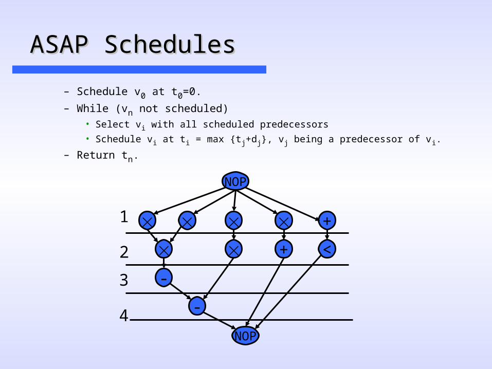
ASAP SchedulesASAP Schedules
– Schedule v0 at t0=0.
– While (vn not scheduled)• Select vi with all scheduled predecessors
• Schedule vi at ti = max {tj+dj}, vj being a predecessor of vi.
– Return tn.
+
NOP
+ <
-
-
NOP
1
2
3
4

ALAP SchedulesALAP Schedules
– Schedule vn at t0=.
– While (v0 not scheduled)
• Select vi with all scheduled successors
• Schedule vi at ti = min {tj-dj}, vj being a succecessor of vi.
+
NOP
+ <
-
-
NOP
1
2
3
4
Resource Constraint SchedulingResource Constraint Scheduling
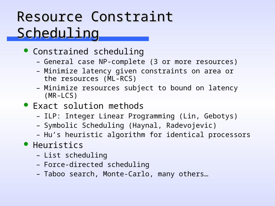
Constrained scheduling– General case NP-complete (3 or more resources)– Minimize latency given constraints on area or
the resources (ML-RCS)– Minimize resources subject to bound on latency (MR-LCS)
Exact solution methods– ILP: Integer Linear Programming (Lin, Gebotys)– Symbolic Scheduling (Haynal, Radevojevic)– Hu’s heuristic algorithm for identical processors
Heuristics– List scheduling– Force-directed scheduling– Taboo search, Monte-Carlo, many others…

Linear ProgrammingLinear Programming
A linear program consists of a set of real variables, a set of linear constraints on the variables and a linear objective function– A set of feasible points, each characterized by a vector of
real values satisfying all the linear constraints may exist.– Because each linear constraint describes a half-space, with
points on one side being feasible, the intersection of the half spaces, if it exists is a convex hull.
– The objective function can be characterized as a set of level planes with the objective increasing along a vector normal to the planes.
– Since the feasible points are convex, a maximal feasible point occurs one or more hull verticies.

Why Linear Programming?Why Linear Programming?

Use binary decision variables– i = 0, 1, ..., n– l = 1, 2, ..., ’+1 ’ given upper-bound on latency – xil = 1 if operation i starts at step l, 0 otherwise.
Set of linear inequalities (constraints),and an objective function (min latency)
Observations:–
– ti = start time of op i.
– is op vi (still) executing at step l?
Simplified ILP FormulationSimplified ILP Formulation
))(),((
0
iLii
Si
Li
Siil
vALAPtvASAPt
tlandtlforx
ill
i xlt
11
l
dlmim
i
x

Start Time vs. Execution TimeStart Time vs. Execution Time
Each operation vi , exactly one start time
If di=1, then the following questions are the same:
– Does operation vi start at step l?
– Is operation vi running at step l?
But if di>1, then the two questions should be
formulated as:– Does operation vi start at step l?
• Does xil = 1 hold?
– Is operation vi running at step l?
• Does the following hold?
11
l
dlmim
i
x

Operation Operation vvii Still Running at Step Still Running at Step l l ??
Is v9 running at step 6?
– Is x9,6 + x9,5 + x9,4 = 1 ?
Note:– Only one (if any) of the above three cases can happen– To meet resource constraints, we have to ask the same question
for ALL steps, and ALL operations of that type
v9
456
x9,4=1
v9
456
x9,5=1
v9
456
x9,6=1
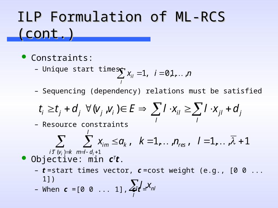
Constraints:– Unique start times:
– Sequencing (dependency) relations must be satisfied
– Resource constraints
Objective: min cTt.– t =start times vector, c =cost weight (e.g., [0 0 ... 1])– When c =[0 0 ... 1], cTt =
ILP Formulation of ML-RCS (cont.)ILP Formulation of ML-RCS (cont.)
l
il nix ,,1,0,1 K
jl
jll
ilijjji dxlxlEvvdtt ),(
1,,1,,,1,)(: 1
KK lnkax reskkvTi
l
dlmim
i i
nll
xl .

ILP ExampleILP Example
First, perform ASAP and ALAP ( = 4)– (we can write the ILP without ASAP and ALAP, but using ASAP and
ALAP will simplify the inequalities)
+
NOP
+ <
-
-
NOP
1
2
3
4
+
NOP
+ <
-
-
NOP
1
2
3
4
v2v1
v3
v4
v5
vn
v6
v7
v8
v9
v10
v11
v2v1
v3
v4
v5
vn
v6
v7 v8
v9
v10
v11
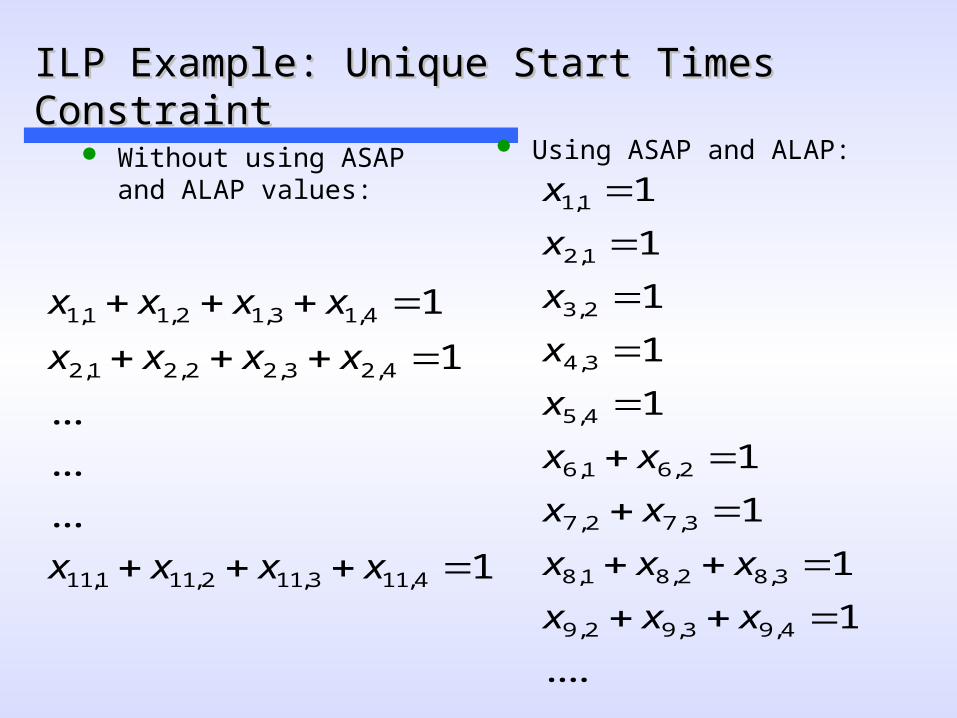
ILP Example: Unique Start Times ConstraintILP Example: Unique Start Times Constraint
Without using ASAP and ALAP values:
Using ASAP and ALAP:
1
...
...
...
1
1
4,113,112,111,11
4,23,22,21,2
4,13,12,11,1
xxxx
xxxx
xxxx
....
1
1
1
1
1
1
1
1
1
4,93,92,9
3,82,81,8
3,72,7
2,61,6
4,5
3,4
2,3
1,2
1,1
xxx
xxx
xx
xx
x
x
x
x
x

ILP Example: Dependency ConstraintsILP Example: Dependency Constraints
Using ASAP and ALAP, the non-trivial inequalities are: (assuming unit delay for + and *)
01.4.3.2.5
01.4.3.2.5
01.3.2.4
01.3.2.4.3.2
01.3.2.4.3.2
01.2.3.2
4,113,112,115,
4,93,92,95,
3,72,74,5
3,102,101,104,113,112,11
3,82,81,84,93,92,9
2,61,63,72,7
xxxx
xxxx
xxx
xxxxxx
xxxxxx
xxxx
n
n

ILP Example: Resource ConstraintsILP Example: Resource Constraints
Resource constraints (assuming 2 adders and 2 multipliers)
Objective: Min Xn,4
2
2
2
2
2
2
2
4,114,94,5
3,113,103,93,4
2,112,102,9
1,10
3,83,7
2,82,72,62,3
1,81,61,21,1
xxx
xxxx
xxx
x
xx
xxxx
xxxx
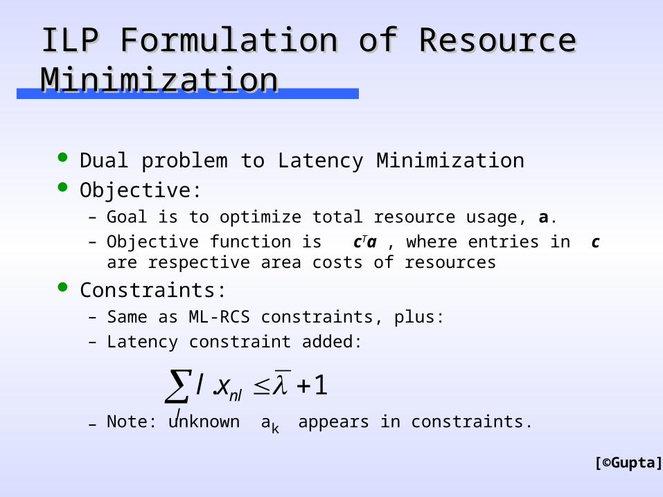
ILP Formulation of Resource MinimizationILP Formulation of Resource Minimization
Dual problem to Latency Minimization Objective:
– Goal is to optimize total resource usage, a.– Objective function is cTa , where entries in c
are respective area costs of resources
Constraints:– Same as ML-RCS constraints, plus:– Latency constraint added:
– Note: unknown ak appears in constraints.
1. nll
xl
[©Gupta]
Hu’s AlgorithmHu’s Algorithm
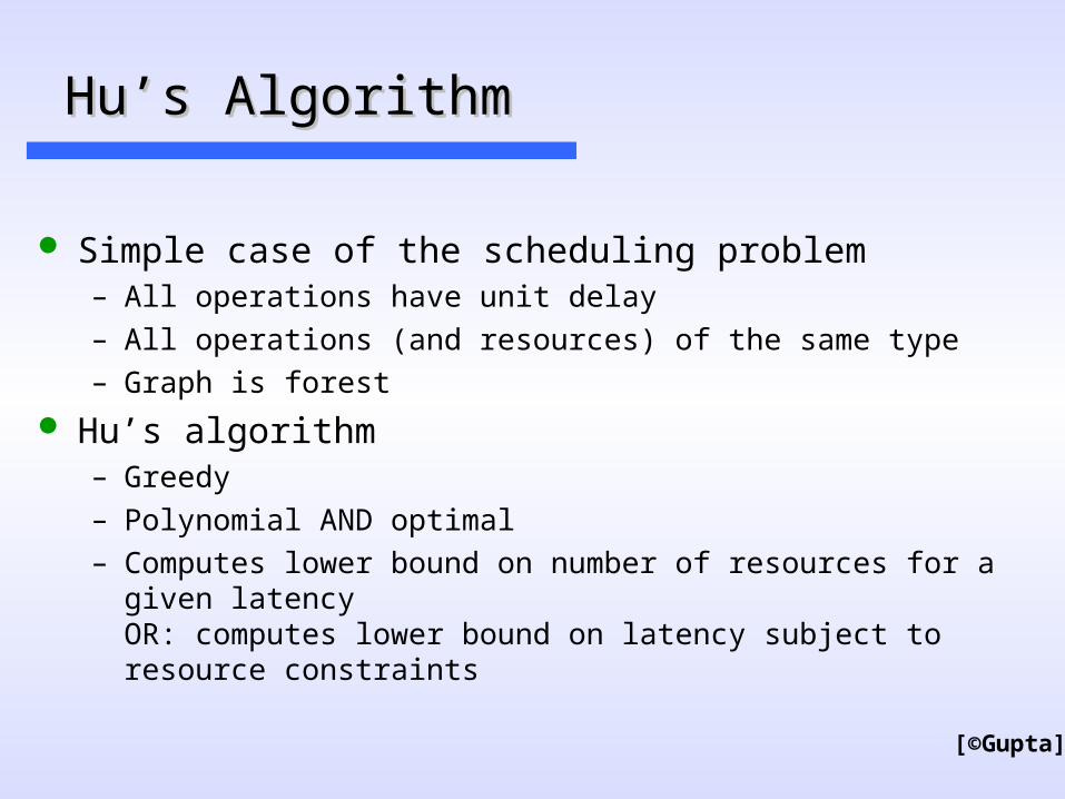
Simple case of the scheduling problem– All operations have unit delay– All operations (and resources) of the same type– Graph is forest
Hu’s algorithm– Greedy– Polynomial AND optimal– Computes lower bound on number of resources for a given latency
OR: computes lower bound on latency subject to resource constraints
[©Gupta]
Basic Idea: Hu’s AlgorithmBasic Idea: Hu’s Algorithm
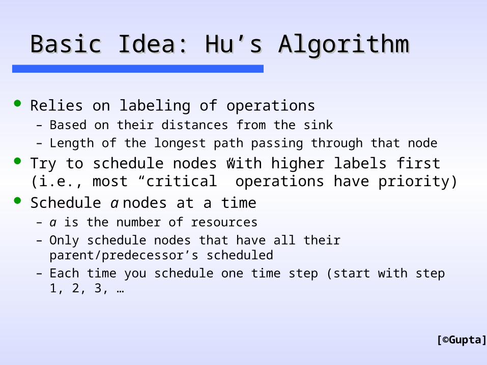
Relies on labeling of operations– Based on their distances from the sink – Length of the longest path passing through that node
Try to schedule nodes with higher labels first(i.e., most “critical” operations have priority)
Schedule a nodes at a time– a is the number of resources– Only schedule nodes that have all their parent/predecessor’s
scheduled– Each time you schedule one time step (start with step 1, 2, 3, …
[©Gupta]
Hu’s Algorithm:Hu’s Algorithm:
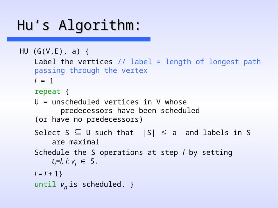
HU (G(V,E), a) {
Label the vertices // label = length of longest pathpassing through the vertex
l = 1
repeat {
U = unscheduled vertices in V whose predecessors have been scheduled
(or have no predecessors)
Select S U such that |S| a and labels in S are maximal
Schedule the S operations at step l by setting ti=l, i: vi S.
l = l + 1}
until vn is scheduled. }

Hu’s Algorithm: ExampleHu’s Algorithm: Example
[©Gupta]
Step 1: Label Vertices (Assume all operations have unit delays):

Hu’s Algorithm: ExampleHu’s Algorithm: Example
[©Gupta]
Find unscheduled vertices with scheduled parents; pick 3 (num. resources) that maximize labels

Hu’s Algorithm: ExampleHu’s Algorithm: Example
[©Gupta]
Repeat until all nodes are scheduled

List SchedulingList Scheduling
Heuristic methods for RCS and LCS– Does NOT guarantee optimum solution
Similar to Hu’s algorithm– Greedy strategy– Operation selection decided by criticality– O(n) time complexity
More general input– Works on general graphs (unlike Hu’s)– Resource constraints on different resource types

List Scheduling Algorithm: ML-RCSList Scheduling Algorithm: ML-RCS
LIST_L (G(V,E), a) {l = 1repeat {
for each resource type k {
Ul,k = available vertices in V
Tl,k = operations in progress.
Select Sk Ul,k such that |Sk| + |Tl,k| ak
Schedule the Sk operations at step l
}l = l + 1
} until vn is scheduled.
}

List Scheduling ExampleList Scheduling Example
[©Gupta]
Assumptions: three multipliers with latency 2; 1 ALU with latency 1

List Scheduling Algorithm: MR-LCSList Scheduling Algorithm: MR-LCS
LIST_R (G(V,E), ’) {a = 1, l = 1
Compute the ALAP times tL.
if t0L < 0
return (not feasible)repeat {
for each resource type k {
Ul,k = available vertices in V.
Compute the slacks { si = tiL - l, vi Ul,k }.
Schedule operations with zero slack, update a
Schedule additional Sk Ul,k under a constraints}l = l + 1}
until vn is scheduled. }

Control Dependency in SchedulingControl Dependency in Scheduling
Practical Programs often have behavior that is dependant on a few conditions. Such conditions are called “control” variables and are usually Boolean or short Enumerations.– Effects incorporated in Data-Flow by making the
dependencies multi-valued, with selection by the dynamic value of some control variable
– Program controls can be modeled by marking every dependency entering or leaving a basic block, using scope and sequencing rules to identify dependent targets
Issue: Controls nest making the number of dependent paths grow exponentially fast– How to avoid blow-up of the problem representation?

CDFG RepresentationCDFG Representation
Operation
Control Dependency
DataDependency
Fork
Join
i2
h1 i1
j1
k1
Resource Class
if Trueif False
j2
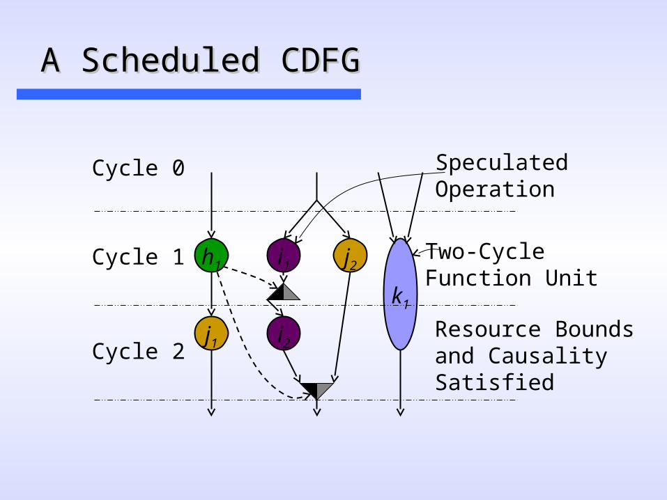
A Scheduled CDFGA Scheduled CDFG
h1
Resource Boundsand CausalitySatisfied
Two-CycleFunction Unit
SpeculatedOperation
i2
i1 j2
j1
k1
Cycle 0
Cycle 1
Cycle 2

0 1
Operations as One-Bit NFAsOperations as One-Bit NFAs
00 Operation unscheduled and remains so
00 11
01
01 Operation scheduled next cycle
11 Operation scheduled and remains so
j1
10 Operation scheduled but result lost

Product of all One-Bit NFAs form Product of all One-Bit NFAs form Scheduling NFAScheduling NFA
Compressed ROBDD representation State represents subset of completed operations Constraints modify transition relation
0 1 0 10 1
h i k….

00 01 11h
00 01 11i
00 01 11j 01
01
Resource BoundsResource Bounds
Operation’s 01 indicates resource use
Resource bounds limit simultaneous 01 in scheduling NFA
01
01
01
01
1101
00 ROBDD representation:
– operations choose bound
– 2boundoperations nodes
– easy to build & compressed
One Resource Unit
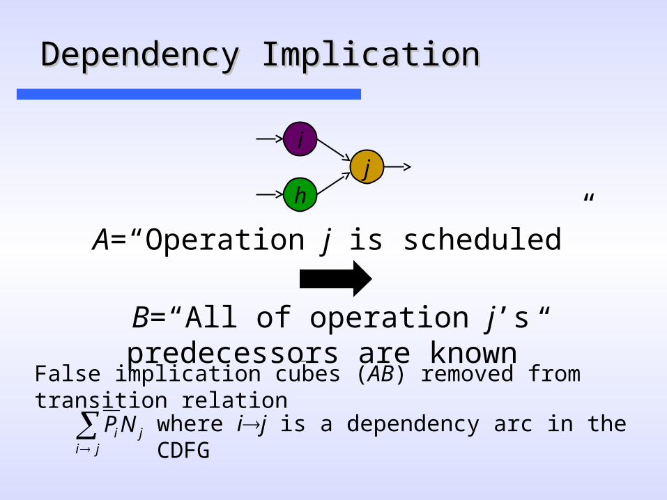
Dependency ImplicationDependency Implication
A=“Operation j is scheduled”
B=“All of operation j’s predecessors are known”
where ij is a dependency arc in the CDFG ji
ji NP
False implication cubes (AB) removed from transition relation
h
ij

i j
h
Valid DFG Scheduling NFAValid DFG Scheduling NFA
Example DFG, 1 resource
NFA transition relation implicitly represents graph
Any path from all operations unknown to all known is a valid schedule
Shortest path is minimum latency schedule
000
i00
ij0
00h
i0h
ijh
000
i00
ij0
00h
i0h
ijh
000
i00
ij0
00h
i0h
ijh
000
i00
ij0
00h
i0h
ijh
000
i00
ij0
00h
i0h
ijh
000
i00
ij0
00h
i0h
ijh
000
i00
ij0
00h
i0h
ijh
000
i00
ij0
00h
i0h
ijh
3
2
1
0
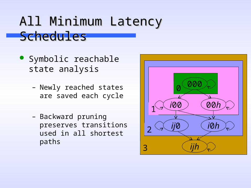
All Minimum Latency SchedulesAll Minimum Latency Schedules
Symbolic reachable state analysis
000
i00
ij0
00h
i0h
ijh
– Newly reached states are saved each cycle
– Backward pruning preserves transitions used in all shortest paths

2
1
0
All Minimum Latency SchedulesAll Minimum Latency Schedules
Symbolic reachable state analysis
000
i00
ij0
00h
i0h
ijh
– Backward pruning preserves transitions used in all shortest paths
– Newly reached states are saved each cycle

1
0
All Minimum Latency SchedulesAll Minimum Latency Schedules
Symbolic reachable state analysis
000
i00
ij0
00h
i0h
ijh
– Backward pruning preserves transitions used in all shortest paths
– Newly reached states are saved each cycle
0
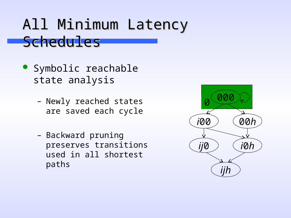
All Minimum Latency SchedulesAll Minimum Latency Schedules
Symbolic reachable state analysis
000
i00
ij0
00h
i0h
ijh
– Backward pruning preserves transitions used in all shortest paths
– Newly reached states are saved each cycle

All Minimum Latency SchedulesAll Minimum Latency Schedules
Symbolic reachable state analysis
000
i00
ij0
00h
i0h
ijh
Not bound to reachable state analysis– Refinements or heuristics to find subset
of shortest paths– Other objectives besides shortest paths
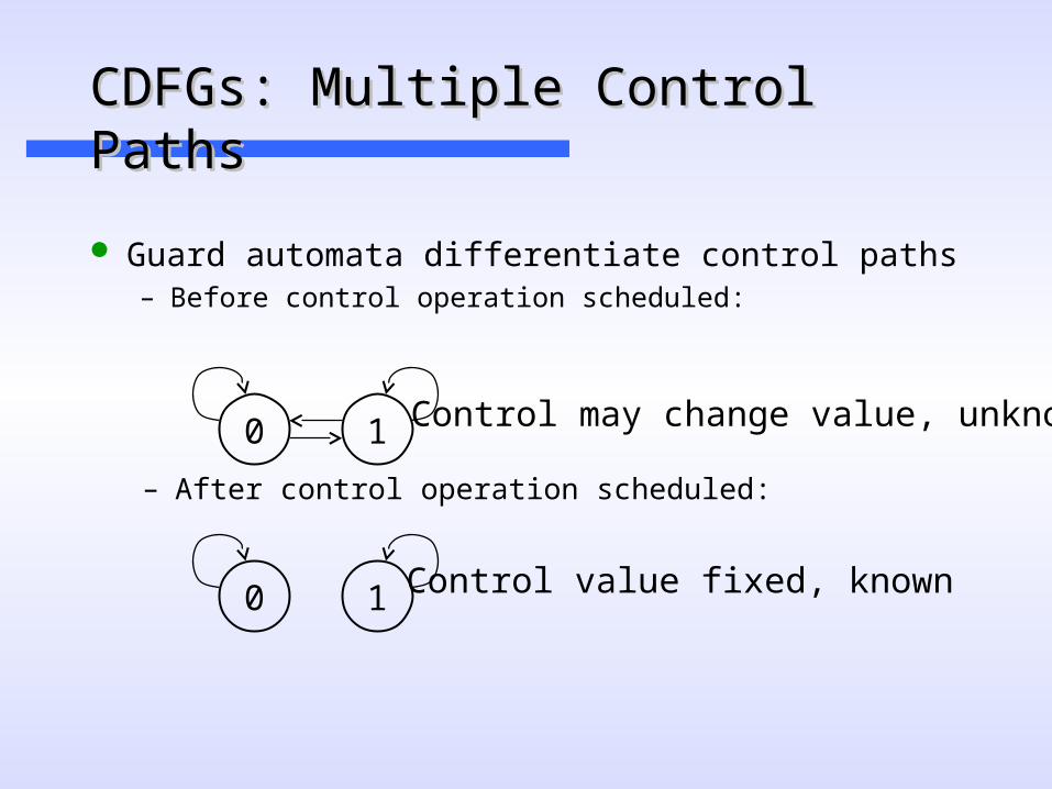
CDFGs: Multiple Control PathsCDFGs: Multiple Control Paths
Guard automata differentiate control paths– Before control operation scheduled:
0 1 Control may change value, unknown
– After control operation scheduled:
0 1 Control value fixed, known
CDFGs: Multiple Control PathsCDFGs: Multiple Control Paths
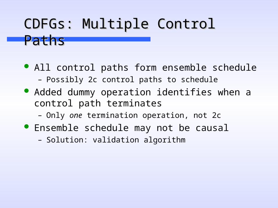
All control paths form ensemble schedule– Possibly 2c control paths to schedule
Added dummy operation identifies when a control path terminates– Only one termination operation, not 2c
Ensemble schedule may not be causal– Solution: validation algorithm

Join Dependency ImplicationJoin Dependency Implication
ij
h
A = “Operation j is scheduled”
B = “The join control resolution is known and all of operation j’s resolved
predecessors are known”

i
j
Operation ExclusionOperation Exclusion
Control unknown– Speculation possible– Resource bounds applicable to both branches
Joint Resource Bounds
?Known
Separate Resource Bounds
Control known– Branch resource bounds mutually exclusive– Other branch’s operations not required

0000
0i00
c000
00j0
ci00
0ij0
c0j0
ci0t
cij0
c0jt
cijt
CDFG ExampleCDFG Example
One green resource
i jc
t
Shortest paths
False termination

Validated CDFG ExampleValidated CDFG Example
Validation algorithm ensures control paths don’t bifurcate before control value is known
0000
0i00
c000
00j0
ci00
0ij0
c0j0
cij0cijt

Validated CDFG ExampleValidated CDFG Example
Validation algorithm ensures control paths don’t bifurcate before control value is known
Pruned for all shortest paths as before
0000
0i00 00j0
ci00 c0j0
cij0cijt

Automata-based Scheduling ConclusionsAutomata-based Scheduling Conclusions
Efficient encoding– No pruning used!– Breadth-first search consolidates
schedules with common histories 000
i00
ij0
00h
i0h
ijh
All valid schedules found– Further refinements and heuristics possible
Despite exact nature, representation growth is minimized– O(<operations>*<cycles>*<controls>)

Construction for Looping DFG’sConstruction for Looping DFG’s
Use trick: 0/1 representation of the MA could be interpreted as 2 mutually exclusive operand productions
Schedule from ~know -> known -> ~known where each 0->1 or 1->0 transition requires a resource.
Since dependencies are on operands, add new dependencies in 1 ->0 sense as well
Idea is to remove all transitions which do not have complete set of known or ~known predecessors for respective sense of operation
So -- get looping DFG automata as nearly same automata as before– preserve efficient representation
Selection of “Minimal Latency” solutions is more difficult
Loop construction: resourcesLoop construction: resources
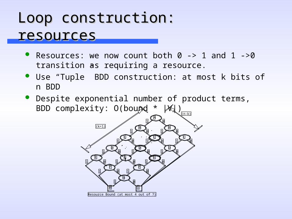
Resources: we now count both 0 -> 1 and 1 ->0 transition as requiring a resource.
Use “Tuple” BDD construction: at most k bits of n BDD Despite exponential number of product terms, BDD complexity:
O(bound * |V|)
0 1
A
B B
C C C
D D D
E E
F F
G
E
(n-k)
(k+1)
1
1 1
1 1 1
1 1 1
1 1 1
1 1
1
0
0 0
0 0 0
0 0 0
0 0 0
0 0
0
Resource Bound (at most 4 out of 7)
Example CAExample CA
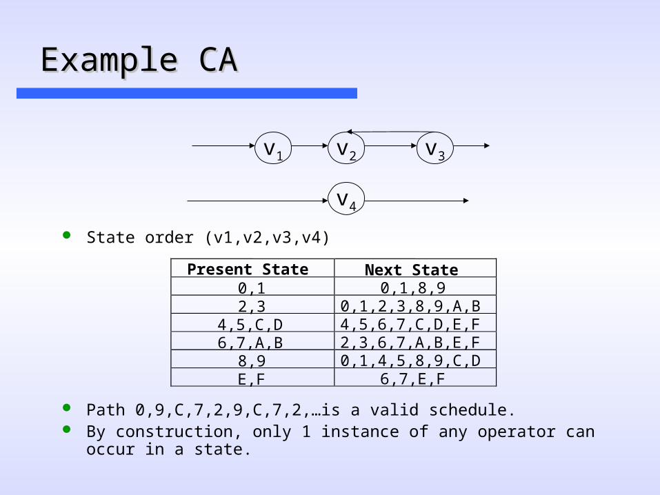
State order (v1,v2,v3,v4)
Path 0,9,C,7,2,9,C,7,2,…is a valid schedule. By construction, only 1 instance of any operator can occur in a state.
v1 v2 v3
v4
Present State Next State0,1 0,1,8,92,3 0,1,2,3,8,9,A,B
4,5,C,D 4,5,6,7,C,D,E,F6,7,A,B 2,3,6,7,A,B,E,F
8,9 0,1,4,5,8,9,C,DE,F 6,7,E,F

Strategy to Find Maximal ThroughputStrategy to Find Maximal Throughput
CA automata construction simple How to find closed subset of paths guaranteeing optimal throughput Could start from known initial state and prune slow paths as before--
but this is not optimal!
Instead: find all reachable states (without resource bounds) Use state set to prune unreachable transitions from CA Choose operator at random to be pinned (marked) Propagate all states with chosen operator until it appears again in
same sense Verify closure of constructed paths by Fixed Point iteration If set is empty -- add one clock to latency and verify again
Result is maximal closed set of paths for which optimal throughput is guaranteed

Maximal Throughput ExampleMaximal Throughput Example
DFG above has closed 3-cycle solution (2 resources) However- average latency is 2.5-cycles (a,d) (b,e) (a,c) (b,d) (c,e) (a,d) … Requires 5 states to implement optimal throughput instance In general, it is possible that a k-cycle closed solution may exist,
even if no k-state solution can be found Current implementation finds all possible k-cycle solutions
a b c
d e
Schedule Exploration: Schedule Exploration: LoopsLoops
Idea: Use partial symbolic traversal to find states bounding minimal latency paths
Latency-- Identify all paths completing cycle in given number of steps
Repeatability-- Fixed Point Algorithm to eliminate all paths which cannot repeat in given latency
Validation-- Ensure all possible control paths are present for each remaining path
Optimization-- Selection of Performance Objective

Kernel Execution Sequence SetKernel Execution Sequence Set
Path from Loop cut to first repeating states
Represents candidates for loop kernel
Loop Kernel
I~
L~k~j~
Loop Cut
i
lkj
a~
d~c~b~
a
dcb

Repeatable Kernel Repeatable Kernel Execution Sequence SetExecution Sequence Set
Fixed-point prunes non-repeating states
Only repeatable loop kernels remain
Paths not all same length
Average latency <= shortest Repeating KernelLoop Cut
Repeatable Loop Kernel
i
lkj
a~
c~b~
a
cb
i~
l~K~j~

Validation IValidation I
Schedule Consists of bundle of compatible paths for each possible future
Not Feasible to identify all schedules
Instead, eliminate all states which do not belong to some ensemble schedule
Fragile since any further pruning requires re-validation
Double fixed point

Validation IIValidation II
Path Divergence -- Control Behavior
Ensure each path is part of some complete set for each control outcome
Ensure that each set is Causal
i
lkj
c~b~
cb
i~
l~k~j~

Loop Cuts and KernelsLoop Cuts and Kernels
Method Covers all Conventional Loop Transformations
Sequential Loop
Loop winding
Loop Pielining
Loop Kernel
Loop Cut
Loop Cut
Loop Kernel
Loop Cut
Loop Kernel
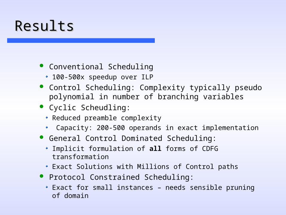
ResultsResults
Conventional Scheduling100-500x speedup over ILP
Control Scheduling: Complexity typically pseudo polynomial in number of branching variables
Cyclic Scheudling:Reduced preamble complexity
Capacity: 200-500 operands in exact implementation General Control Dominated Scheduling:
Implicit formulation of all forms of CDFG transformation
Exact Solutions with Millions of Control paths Protocol Constrained Scheduling:
Exact for small instances – needs sensible pruning of domain
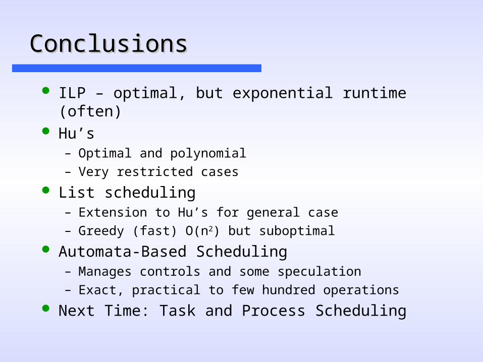
ConclusionsConclusions
ILP – optimal, but exponential runtime (often) Hu’s
– Optimal and polynomial– Very restricted cases
List scheduling– Extension to Hu’s for general case– Greedy (fast) O(n2) but suboptimal
Automata-Based Scheduling– Manages controls and some speculation– Exact, practical to few hundred operations
Next Time: Task and Process Scheduling