Lecture 35 Soil Physics, Moisture Transfer in Soils, …...Biometeorology, ESPM 129 1 Lecture 35...

Biometeorology, ESPM 129

1

Lecture 35 Soil Physics, Moisture Transfer in Soils, Part 2 December 10, 2014 Instructor: Dennis Baldocchi Professor of Biometeorology Ecosystem Science Division Department of Environmental Science, Policy and Management 345 Hilgard Hall University of California, Berkeley Berkeley, CA 94720 Topics 1. Theory, Moisture Transfer

a. Moisture transfer, Darcy’s Law and the Richard’s Equation Soil Release curve.

c. Force Restore models, Bucket models d. Role of different boundary conditions e. Evaporation models

f. CO2 diffusion models 2. Observations, Moisture profiles a. Seasonal patterns b. Influence of soil texture 3. Soil Evaporation

a. measurements b. model calculations

34.1 INTRODUCTION The soil is the reservoir for moisture that is available to roots. How much moisture it contains and the rate that water is lost from the soil depends on its texture, physical/hydraulic capacity and the activity of plant contained within it and the extent of their root system. The presence or absence of moisture and active biology in soils affects how it weathers (Jenny 1994). To understand changes in soil moisture we must start with an understanding of the sources and losses of water.


2

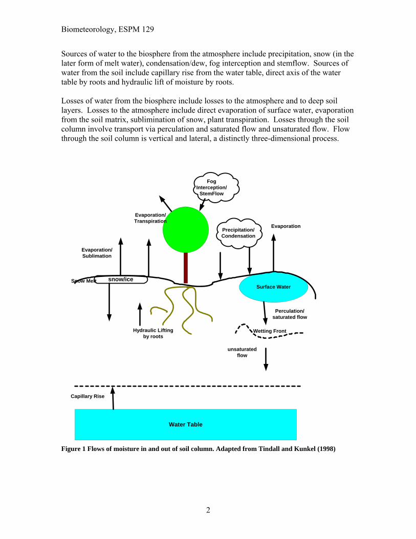
Sources of water to the biosphere from the atmosphere include precipitation, snow (in the later form of melt water), condensation/dew, fog interception and stemflow. Sources of water from the soil include capillary rise from the water table, direct axis of the water table by roots and hydraulic lift of moisture by roots. Losses of water from the biosphere include losses to the atmosphere and to deep soil layers. Losses to the atmosphere include direct evaporation of surface water, evaporation from the soil matrix, sublimination of snow, plant transpiration. Losses through the soil column involve transport via perculation and saturated flow and unsaturated flow. Flow through the soil column is vertical and lateral, a distinctly three-dimensional process.

Figure 1 Flows of moisture in and out of soil column. Adapted from Tindall and Kunkel (1998)

Water Table

Surface Water

snow/ice

Capillary Rise

Evaporation/Sublimation

Wetting Front

Precipitation/Condensation

Evaporation

Perculation/saturated flow

unsaturatedflow

Evaporation/Transpiration

Snow Melt

Hydraulic Liftingby roots

FogInterception/

StemFlow


3

A thermodynamic quantity, soil water potential, is used to describe soil hydrodynamics. The total soil water potential is the amount of work done, per unit quantity of pure water, to transport an infinitesimal amount of water from a pool of pure water. The process is isothermal and a reference pressure (Tyndall and Kunkel, 2000). The components of soil water potential for shallow soils are: Gravitational potential: The force of gravity exerted on a water column produces the gravitation potential. The gravitation potential is related to the work done to transport water from one pool to another, as when lifting a column of water up the xylem of a tree: g l gz

Turgor or pressure potential: Water potential exerted by the pressure or weight of water

p

w

P

Vapor potential: v vs

R Te

e ln( )

R is the universal gas constant Matric potential: It is water potential due to attraction between water and soils. Adhesive and cohesive forces bind water to soil particles (Campbell and Norman, 1999). These interactions reduce the potential of water, giving it a negative sign. m

baw~ Osmotic potential: Osmotic potential arises from the dilution of solutes in water, eg salts, sugars etc. For the osmotic potential to drive water flow, a semi-permeable membrane must separate two bodies of water, such as cells, and pools of water. o c vRT c is the concentration, is the osmotic coefficient and is the number of ions per mole (Campbell and Norman 1998). The total water potential is thus:


4

p o g m

Which components are significant or not depends on the system we are studying (e.g. Baver et al, 1976). Water potential is expressed as energy (kg m2 s-2) per unit volume (m-3), giving it units of kg m-1 s-2, which is equivalent to pressure units, or force per unit area, kg m s-2 m-2). E/V = F x/V = F/A=P In other instances pressure potentials may be normalized by water density

|massw

P

(kg m-1 s-2) * (m3 kg-1)

We know the mass of water is 1000 kg = m3 and water is incompressible, we can substitute mass for density, effectively 1 J/kg = 1 kPa Soil-Water-Plant Relations (apolplast) o m Osmotic and matric potential are important for plant-water relations and water movement in the apoplast and through the xylem. Gravimetric potential is negligible as the suction needed to raise water, typically 1 m is less than 0.1 bar. Organisms, cells (symplast): p o

Inside cells turgor potential (eg pressure potential) and osmotic potentials are most important Unsaturated Flow: g m

Gravitational and matrix potential are dominant Saturated Flow p g

Pressure and gravity are the main components driving water flow in saturated soils. The pressure term includes overburden effects. At a point a point beneath the water table, the


5

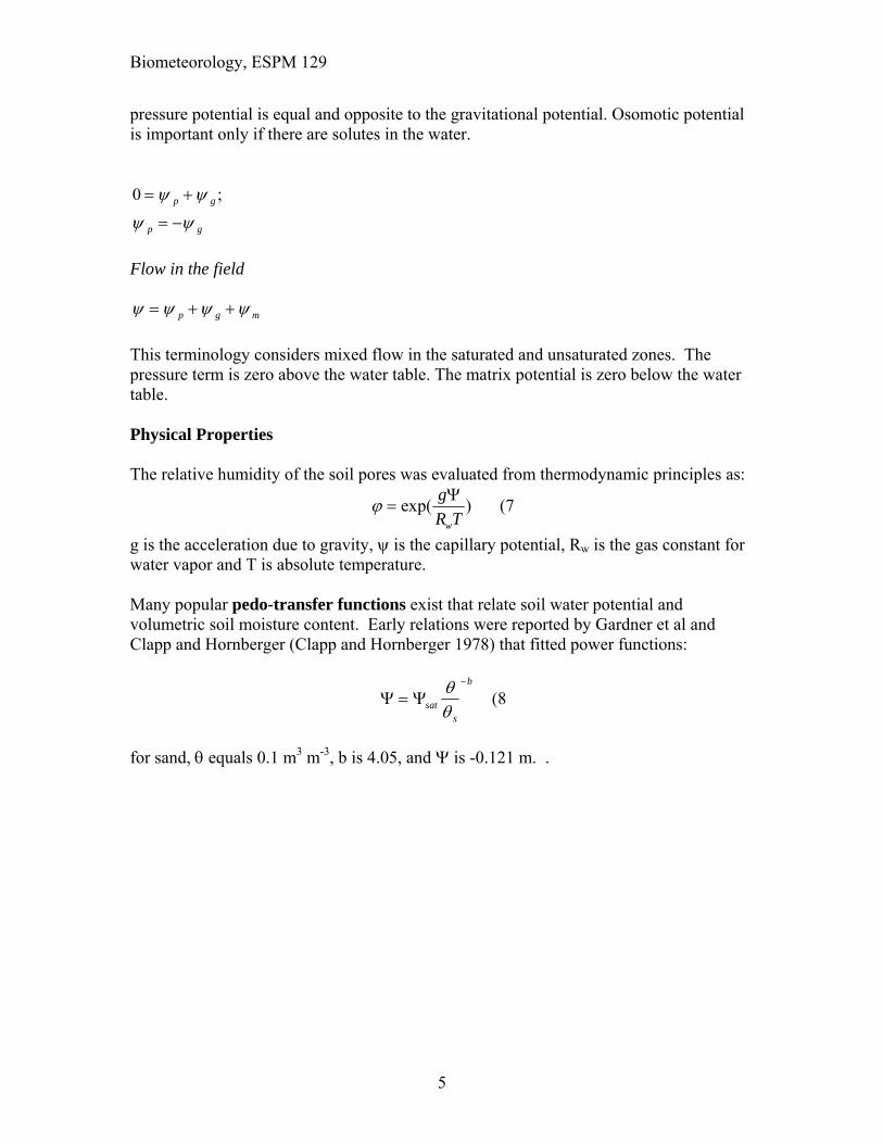
pressure potential is equal and opposite to the gravitational potential. Osomotic potential is important only if there are solutes in the water. 0

p g

p g

;

Flow in the field p g m

This terminology considers mixed flow in the saturated and unsaturated zones. The pressure term is zero above the water table. The matrix potential is zero below the water table. Physical Properties The relative humidity of the soil pores was evaluated from thermodynamic principles as:

exp( )g

R Tw

(7

g is the acceleration due to gravity, is the capillary potential, Rw is the gas constant for water vapor and T is absolute temperature. Many popular pedo-transfer functions exist that relate soil water potential and volumetric soil moisture content. Early relations were reported by Gardner et al and Clapp and Hornberger (Clapp and Hornberger 1978) that fitted power functions:

sats

b

(8

for sand, equals 0.1 m3 m-3, b is 4.05, and is -0.121 m. .


6

Figure 2 Soil moisture retention using equation of Gardner

Table 1 Important physical and hydraulic properties of soils include their textural fractions (silt/clay/sand, the hydraulic conductivity (K) and the volumetric water contents at field capacity (-0.33 bar) and wilting point (-15 bars) (Rawls et al., 1992; Campbell and Norman, 1998)

Texture silt clay b Ks J/kg kg s m-3 M3 m-3 m3 m-3 Sand 0.05 0.03 0.7 1.7 0.0058 0.09 0.03 loamy sand 0.12 0.07 0.9 2.1 0.0017 0.13 0.06 sandy loam 0.25 0.10 1.5 3.1 0.00072 0.21 0.1 Loam 0.4 0.18 1.1 4.5 0.00037 0.27 0.12 silt loam 0.65 0.15 2.1 4.7 0.00019 0.33 0.13 sandy clay loam 0.13 0.27 2.8 4 0.00012 0.26 0.15 clay loam 0.34 0.34 2.6 5.2 0.000064 0.32 0.2 silty clay loam 0.58 0.33 3.3 6.6 0.000042 0.37 0.32 sandy clay 0.07 0.40 2.9 6 0.000033 0.34 0.24 silty clay 0.45 0.45 3.4 7.9 0.000025 0.39 0.25 clay 0.20 0.60 3.7 7.6 0.000017 0.4 0.27

Volumetric Soil Moisture Content

0.0 0.2 0.4 0.6 0.8 1.0

Soi

l Wat

er P

oten

tial (

m),

0.1

1

10

100

1000

10000

sand loam clay


7

Next we see how different soils range between field capacity and wilting point. Note how peat soils become stressed at vary high water contents!

Sandloamy sand

sandy loam

sandy clay loam Loamclay loam

silt loamsandy clay

silty clay loamsilty clay clay peat

Vol

ume

tric

wat

er c

on

ten

t (m

3 m-3

)

0.0

0.2

0.4

0.6

0.8

1.0

field capacity permanent wilting point


8

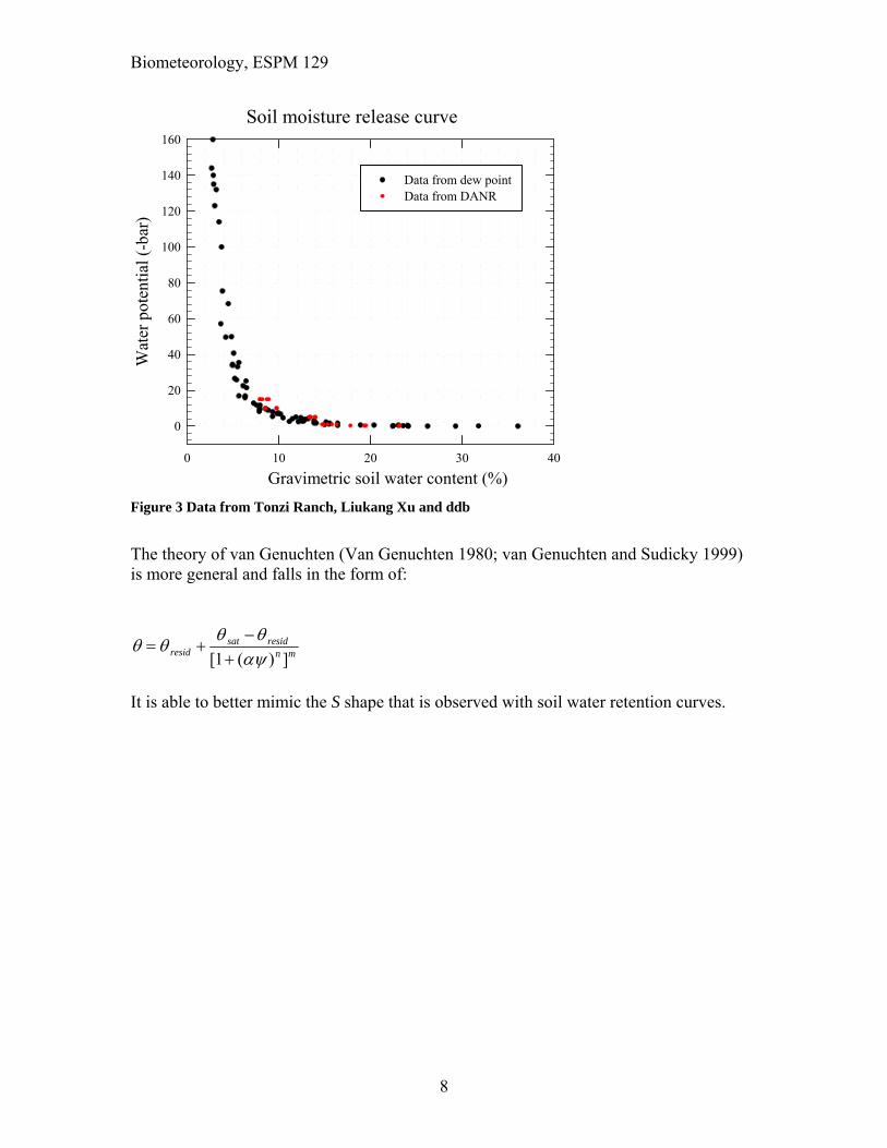
Soil moisture release curve

Gravimetric soil water content (%) 0 10 20 30 40

Wat

er p

oten

tial (

-bar

)

0

20

40

60

80

100

120

140

160

Data from dew point Data from DANR

Figure 3 Data from Tonzi Ranch, Liukang Xu and ddb

The theory of van Genuchten (Van Genuchten 1980; van Genuchten and Sudicky 1999) is more general and falls in the form of:

residsat resid

n m[ ( ) ]1

It is able to better mimic the S shape that is observed with soil water retention curves.


9

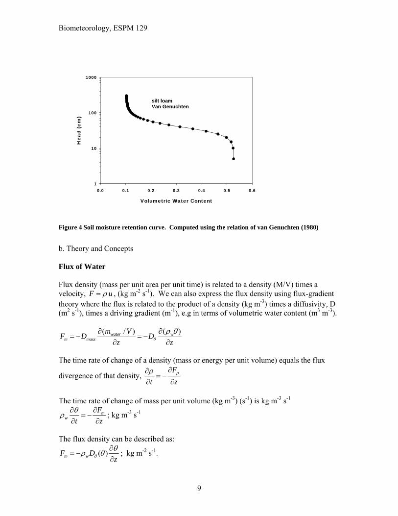
Figure 4 Soil moisture retention curve. Computed using the relation of van Genuchten (1980)

b. Theory and Concepts Flux of Water Flux density (mass per unit area per unit time) is related to a density (M/V) times a velocity, F u , (kg m-2 s-1). We can also express the flux density using flux-gradient theory where the flux is related to the product of a density (kg m-3) times a diffusivity, D (m2 s-1), times a driving gradient (m-1), e.g in terms of volumetric water content (m3 m-3).

( / ) ( )water wm mass

m VF D D

z z

The time rate of change of a density (mass or energy per unit volume) equals the flux

divergence of that density, F

t z

The time rate of change of mass per unit volume (kg m-3) (s-1)

is kg m-3 s-1

mw

F

t z

; kg m-3 s-1

The flux density can be described as:

( )m wF Dz

; kg m-2 s-1.

Volumetric Water Content

0.0 0.1 0.2 0.3 0.4 0.5 0.6

Hea

d (c

m)

1

10

100

1000

silt loamVan Genuchten


10

Re-substitution of the flux equation into the conservation equation produces:

w w h

FD

t z z z

If normalized by w we have a simple budget equation for volumetric water content:

wh

F

Dt z z z

When studying water transfer, water potential tends to be the currency defining the driving gradient. Here, the flux density of Energy is a product of the energy density (J/V) times a velocity: (J m-3) m s-1 =J m-2 s-1= (kg m2 s-2) m-2 s-1 = kg s-3 = Pa m s-1

( )wF Dz

If I was to start from first principles I’d define a flux in terms of water potential

dF D

dz

And solve for water potential with the advection-diffusion equation, or conservation budget

2

2

( )DF Dz Dt z z z z z

A difficulty/complexity/confusion arises because:

1. the continuity equation solves for water potential, but soil moisture tends to be

measured in terms of volumetric water content and inputs and outflows are measured

in terms of velocity per unit area, eg mm d‐1.

2. The water transfer equations in the hydraulic literature are typically expressed in terms

of a conductivity, K, instead of and diffusivity, D, which is counter‐intuitive based on

equations in the atmospheric literature.

3. Different flux equations have different units of K (m s‐1 vs kg s m‐3).


11

4. Some flux equations express the driving potential is terms of head, h, rather than

pressure and others express the driving potential in terms of Energy normalized by

mass, which produce pressure units too.

Darcy’s Law One of the earliest and most applicable theories of soil moisture through soils is attributed to Henry Darcy (1803-1858), a French scientist working for Napoleon (Philip 1995) Darcy performed experiments on water transfer through a bed of sand and derived what came to be known as Darcy’s Law. The volume of water passing through a bed of sand per unit time is a function of the cross-sectional area, A, the thickness of the bed, L, the depth of water on top of the bed, h, and the hydraulic conductivity of the sand, K:

Q KA h

L

In terms of a flux density

qQ

A

V

AtK

h

L

(volume of water crossing a known area in a given time)

The hydraulic conductivity is defined from experiment as:

KVL

At h

Civil and environmental engineers and soil scientists often measure head, h, instead of water potential, so Darcy’s law is often presented in this form:

q Kh z

z

Kh

zK h

( )( )

( ) ( )

q KP

sK

P

sg

z

sh t

( )

The time rate of change of volumetric water content can be expressed in terms of Fick’s second law.

LNM

OQP

t z

K hh

zK h S( ) ( )


12

We add a term S, which represents sources and sinks, such as root uptake or hydraulic lift by plants. Boundary conditions for assessing water content in soils the top and bottom layers. At the top soil content depends upon infiltration, transpiration and evaporation from the soil. At the bottom, one needs to know the water table. Darcy's Law is valid for low Reynolds numbers, where flow is laminar and viscous forces dominate (Re <1). Darcy’s law may be violated in karst limestone and dolomite soils. Darcy’s law also fails in dense clay soils, which have low permeability. The conventional form of Darcy’s Law does not work in the Vadose Zone, the unsaturated soil zone. Water transfer through unsaturated soils is very complex, as soils contain both small and large size pores. Large pores will form from cracks, earthworm or animal holes, and roots. Macro pores can be routes of preferential flow. In unsaturated soils large pores drain first, increasing the potential difference. But a paradox is observed as water flow rates diminish because small pores, which remain wet, are pore conductors of water. The path of water transfer also becomes more tortuous as the soil dries. One can only account for diminishing flow rates with increasing water potential gradients by the co-occurrence of a diminishing hydraulic conductivity, K. Let’s start with the fundamental equations describing the flux of water and re-derive the budget equations and numerical schemes with a consistent form of K that can be evaluated with standard pedotransfer functions and applied correctly to the conservation equation. Darcy’s Law says a flux of water is defined as the product of a hydraulic conductivity and a water potential gradient. Discharge, volume of water per unit time in terms of a pressure or head gradient is:

P hQ A KA

z z

h is head, m

w

Ph z

g

P is pressure, F/A, Pa = kg m‐1 s‐2 A is area, m2 K is conductivity, m s‐1

is permeability, m2

is dynamic viscosity, kg m‐1 s‐1


13

Q is the Discharge of water per unit area (m s‐1)

wh

gQ P h hq K

A z z z

wh

gK

; (m2) (kg m-3) (m s-2)(kg-1 m s) = m s-1

And mass flow of water is

ww w w h w

gP h hF q K

z z z

kg m-2 s-1 = (kg m-3) (m2) (kg-1 m s) (kg m-1 s-2) (m-1) Campbell defines a mass flux as follows:

|massdF K

dz

(kg s m-3) (J/kg) (m-1) = J s m-4 = kg m2 s-2 = kg m-2 s-1 Consequently, the hydraulic conductivities used by Campbell, K , and Darcy, hK , are

not equal and have different units. Let’s try and resolve and reconcile this difference. First, let’s examine all the forms of the flux equation. They may have different drivers and rate factors, but they all must produce a mass flux with units of kg m-2 s-1:

|w mass

w w w h w w w

gP h hF q K

z z z z

From these equations we can deduce several definitions for hydraulic conductivities. The conductivity used by Campbell has units of kg m-3 s and must only be applied against a water potential normalized by mass. This conductivity can be defined as:

w wK

; (kg m-3)(kg m-3) m2 (kg-1 m s) = kg m-3 s

The hydraulic conductivity used in the Richards Equation and has velocity units and must only be applied against head. It can be deduced to equal:

wh

gK

; (m2) (kg m-3) (m s-2) (kg-1 m s) = m s-1

So it is clear that hK K .


14

Next let’s relate them to one another:

ww w h

wh

gK K

K Kg

So the mass flux equation can be re-written in terms of Kh as:

| |mass w mass

w w h h

hF q K K K

z z g z

It is also critical to recognize that one cannot estimate the mass flux by multiplying Kh times the pressure or water potential gradient:

w w h w h

PF q K K

z z

But I want to express the fluxes in terms of and used pedotransfer functions for Kh. With substitution it should be

w h hw w w h w w

w

g K Kh h PF q K

z z z g z g z

So the form of the water flux density equation I want to work with is:

hw

KF

g z

; (m s-1)(m-1 s2)(kg m-1 s-2)(m-1) = kg m-2 s-1

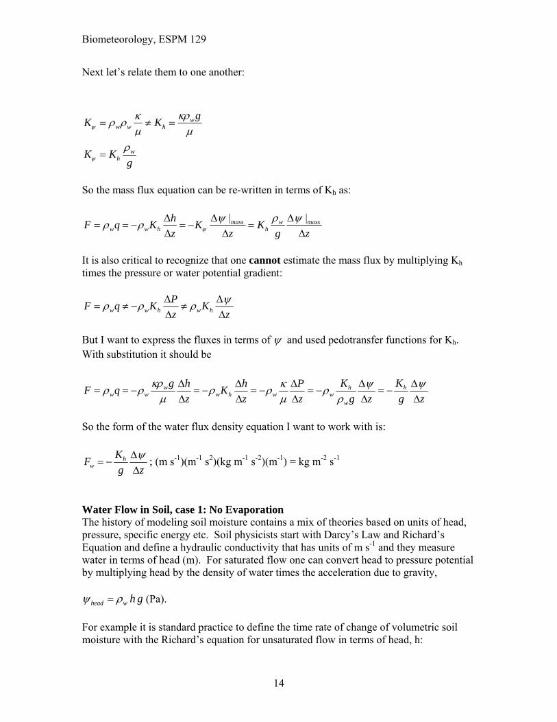
Water Flow in Soil, case 1: No Evaporation The history of modeling soil moisture contains a mix of theories based on units of head, pressure, specific energy etc. Soil physicists start with Darcy’s Law and Richard’s Equation and define a hydraulic conductivity that has units of m s-1 and they measure water in terms of head (m). For saturated flow one can convert head to pressure potential by multiplying head by the density of water times the acceleration due to gravity,

head w h g (Pa).

For example it is standard practice to define the time rate of change of volumetric soil moisture with the Richard’s equation for unsaturated flow in terms of head, h:


15

~m g w wg h g z

~w

h zg

Here I am considering z as the depth relative to the soil surface. So z is negative when it

is below the ground and it is positive when above the ground.

In some applications you’ll see

~m g w wg h g z

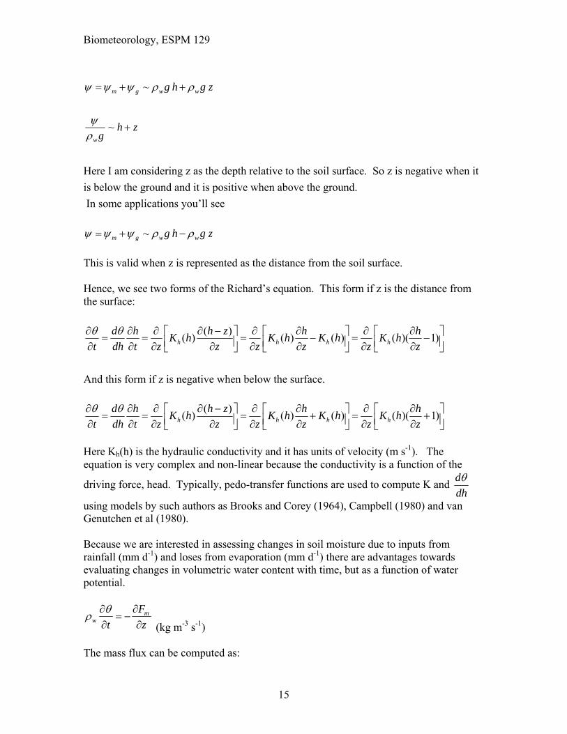
This is valid when z is represented as the distance from the soil surface. Hence, we see two forms of the Richard’s equation. This form if z is the distance from the surface:

( )

( ) ( ) ( ) ( )( 1)h h h h

d h h z h hK h K h K h K h

t dh t z z z z z z

And this form if z is negative when below the surface.

( )( ) ( ) ( ) ( )( 1)h h h h

d h h z h hK h K h K h K h

t dh t z z z z z z

Here Kh(h) is the hydraulic conductivity and it has units of velocity (m s-1). The equation is very complex and non-linear because the conductivity is a function of the

driving force, head. Typically, pedo-transfer functions are used to compute K and d

dh

using models by such authors as Brooks and Corey (1964), Campbell (1980) and van Genutchen et al (1980). Because we are interested in assessing changes in soil moisture due to inputs from rainfall (mm d-1) and loses from evaporation (mm d-1) there are advantages towards evaluating changes in volumetric water content with time, but as a function of water potential.

mw

F

t z

(kg m-3 s-1)

The mass flux can be computed as:


16

hm

KF

g z

And on substitution we have

( )

[ ]hw

K

t z g z

And normalizing by water density produces:

( )

[ ]h

w

K

t z g z

; (m s-1)(kg m-1 s-2) (m-1) (m3 kg-1) (s2 m-1) (m-1)= s-1

We want to explicitly consider effects of matrix and gravitational potential. Replacing

~ m g

The gravitational potential is computed as:

g wgz

But I need to be careful about sign convention because I am working in z units where 0 is

the soil surface and depths below the surface have a negative sign. Gravitational water

potential is positive if above a reference level and is negative if below a reference level.

g wgz

And rearranging terms produces

( ) ( )

[ ]

( ) ( )[ ]

( )[ ( ) ]

gh m h

w w

h m w h

w w

h mh

w

dK d K

t z g dz g dz

K d g K d z

z g dz g dz

K dK

z g dz

s-1

Simplifying to:


17

( )[ ( ) ]h m

hw

K dK

t z g dz

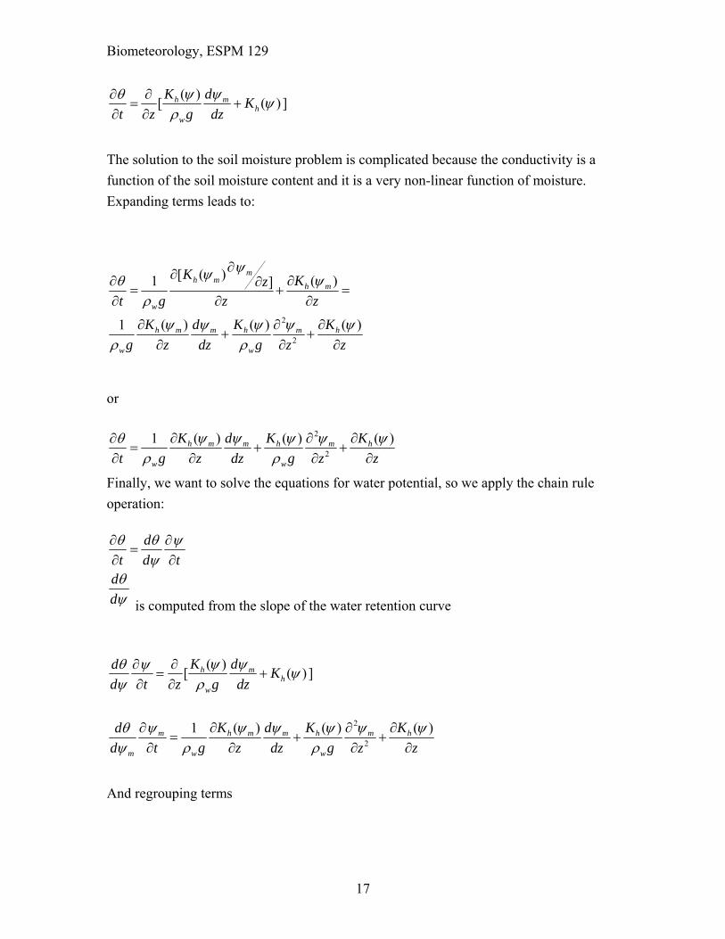
The solution to the soil moisture problem is complicated because the conductivity is a

function of the soil moisture content and it is a very non-linear function of moisture.

Expanding terms leads to:

2

2

[ ( ) ( )1 ]

( ) ( ) ( )1

mh m

h m

w

h m m h m h

w w

K Kzt g z z

K d K K

g z dz g z z

or

2

2

( ) ( ) ( )1 h m m h m h

w w

K d K K

t g z dz g z z

Finally, we want to solve the equations for water potential, so we apply the chain rule

operation:

d

t d t

d

d

is computed from the slope of the water retention curve

( )

[ ( ) ]h mh

w

K ddK

d t z g dz

2

2

( ) ( ) ( )1m h m m h m h

m w w

K d K Kd

d t g z dz g z z

And regrouping terms


18

2

2

( ) ( ) 1[ 1]m h m h m m

m w w

d K K d

d t t g z z g dz

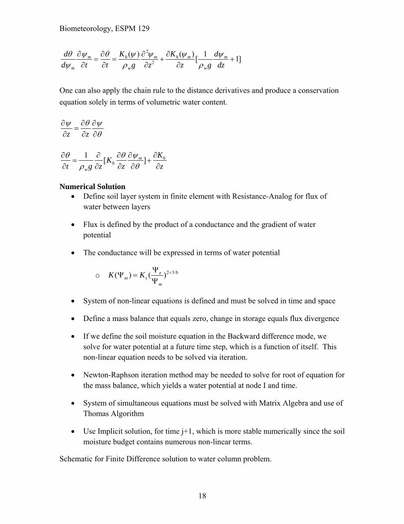
One can also apply the chain rule to the distance derivatives and produce a conservation

equation solely in terms of volumetric water content.

z z

1[ ]m h

hw

KK

t g z z z

Numerical Solution

Define soil layer system in finite element with Resistance-Analog for flux of water between layers

Flux is defined by the product of a conductance and the gradient of water potential

The conductance will be expressed in terms of water potential

o 2 3/( ) ( ) bem s

m

K K

System of non-linear equations is defined and must be solved in time and space

Define a mass balance that equals zero, change in storage equals flux divergence

If we define the soil moisture equation in the Backward difference mode, we solve for water potential at a future time step, which is a function of itself. This non-linear equation needs to be solved via iteration.

Newton-Raphson iteration method may be needed to solve for root of equation for the mass balance, which yields a water potential at node I and time.

System of simultaneous equations must be solved with Matrix Algebra and use of Thomas Algorithm

Use Implicit solution, for time j+1, which is more stable numerically since the soil moisture budget contains numerous non-linear terms.

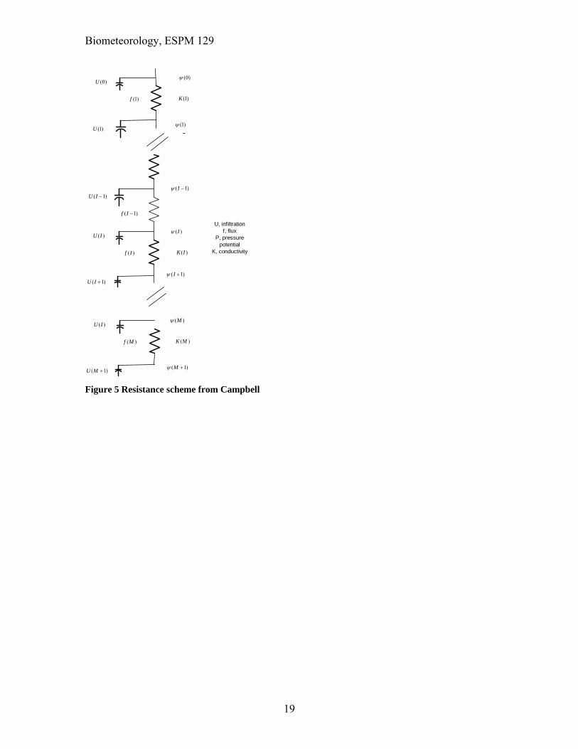
Schematic for Finite Difference solution to water column problem.


19

( )I

( 1)I

( 1)I

(1)K

( )K I

( 1)f I

( )f I

( 1)U I

( )U I

( 1)U I

U, infiltrationf, flux

P, pressurepotential

K, conductivity

(0)

(1)

(1)f

(1)U

( )M

( 1)M

( )K M( )f M

( )U I

( 1)U M

(0)U

Figure 5 Resistance scheme from Campbell


20

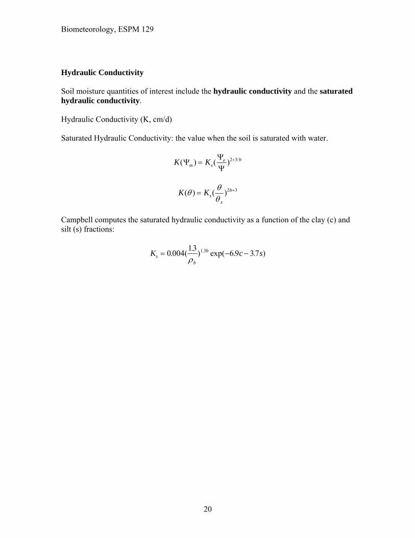
Hydraulic Conductivity Soil moisture quantities of interest include the hydraulic conductivity and the saturated hydraulic conductivity. Hydraulic Conductivity (K, cm/d) Saturated Hydraulic Conductivity: the value when the soil is saturated with water.

K Km se b( ) ( ) /

2 3

K Kss

b( ) ( )

2 3

Campbell computes the saturated hydraulic conductivity as a function of the clay (c) and silt (s) fractions:

K c ssb

b 0 00413

6 9 371 3. (.

) exp( . . ).


21

Figure 6 Hydraulic conductivity as a function of soil testure and volumetric water content. Computed with the Equations of Campbell.

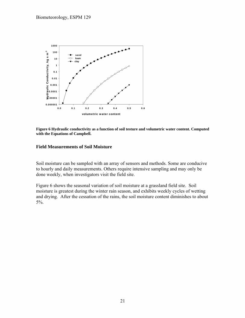
Field Measurements of Soil Moisture Soil moisture can be sampled with an array of sensors and methods. Some are conducive to hourly and daily measurements. Others require intensive sampling and may only be done weekly, when investigators visit the field site. Figure 6 shows the seasonal variation of soil moisture at a grassland field site. Soil moisture is greatest during the winter rain season, and exhibits weekly cycles of wetting and drying. After the cessation of the rains, the soil moisture content diminishes to about 5%.

volumetric water content

0.0 0.1 0.2 0.3 0.4 0.5 0.6

Hyd

raul

ic C

ondu

ctiv

ity,

kg

s m

-3

0.000001

0.00001

0.0001

0.001

0.01

0.1

1

10

100

1000

sand loam clay


22

day

0 50 100 150 200 250 300 350

Soi

l moi

stur

e (c

m3 c

m-3

)

0.0

0.1

0.2

0.3

0.4

0.5

Daily SamplingWeekly Sampling

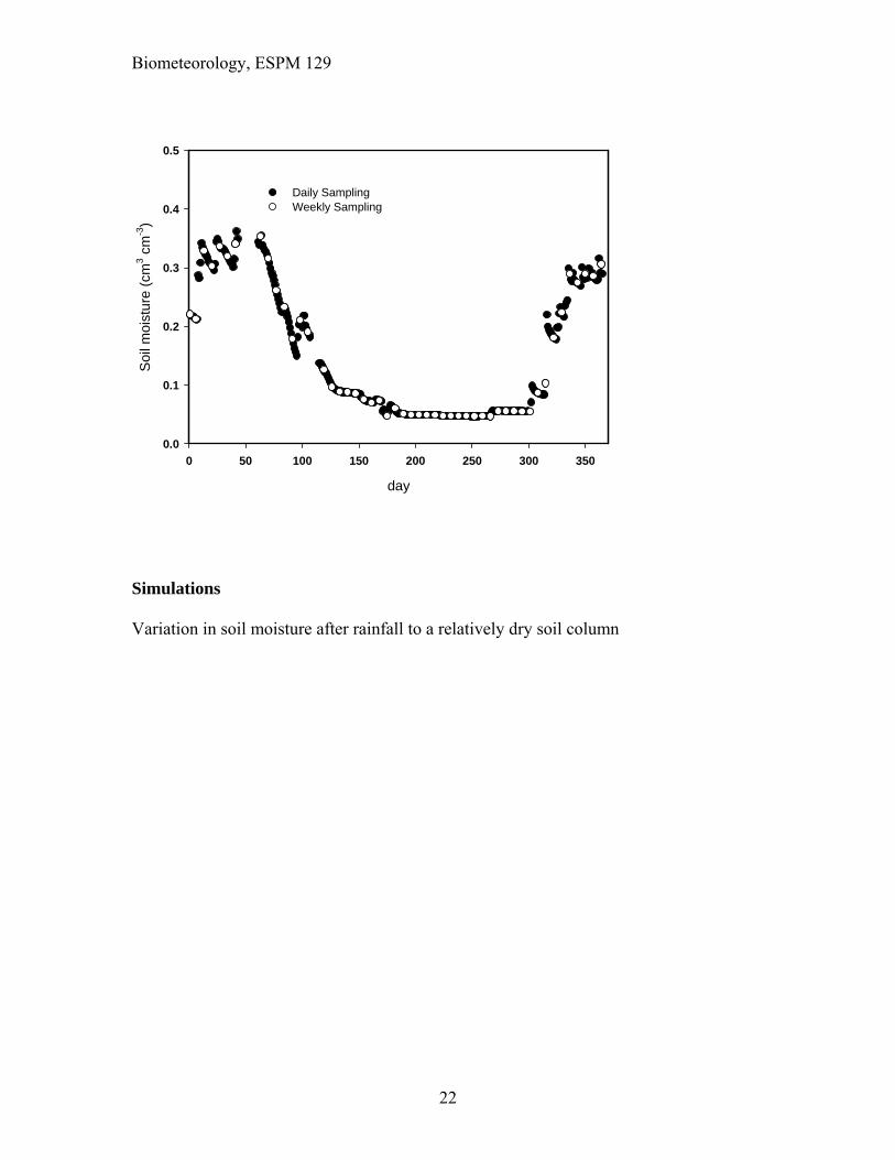
Simulations Variation in soil moisture after rainfall to a relatively dry soil column


23


0.0 0.1 0.2 0.3 0.4 0.5

-z (

m)

0.01

0.1

1

10

T = 1 hourT = 2 hourT = 12 hourT = 24 hours T = 48 hours T= 96 hoursT = 192 hoursT= 382 hours

Change in soil moisture after rain from a soil that has a distributed root system and is transpiring and evaporating.


0.0 0.1 0.2 0.3 0.4 0.5

-z (

m)

0.01

0.1

1

10

T = 1 hourT = 2 hourT = 12 hourT = 24 hours T = 48 hours T= 96 hours

ppt 25 mm/day on day 1; et 5 mm/day; Root Uptake


24

Gaseous Diffusion Through Soils Diffusion and production of trace gases (eg CO2) in the soil

c

tD

c

z

2

2

ε is the free air porosity of the soil, D is the molecular diffusivity and φ is the production rate (Amundson, 1998). At steady state there is a balance between the production rate and the diffusion flux divergence:

Dc

z

2

2

Using a no flux lower boundary condition (dc/dz =0 at L and C at 0 equals the atmospheric value, then

CD

Lzz

Cs

atm

( )2

2

Such a calculation is useful for giving one some idea of the build up of CO2 in the soil based on the production rate, depth and molecular diffusivity.


25


26

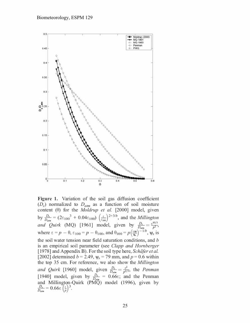
Figure 7after Suwa et al 2004 GCB

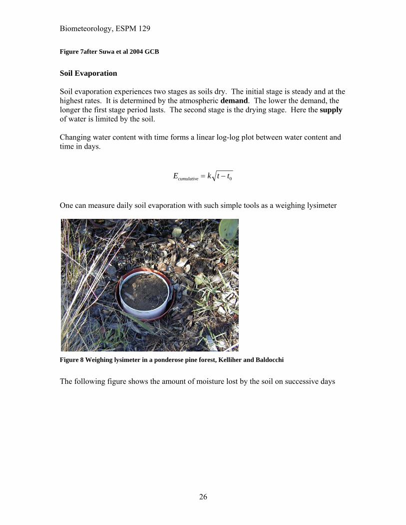
Soil Evaporation Soil evaporation experiences two stages as soils dry. The initial stage is steady and at the highest rates. It is determined by the atmospheric demand. The lower the demand, the longer the first stage period lasts. The second stage is the drying stage. Here the supply of water is limited by the soil. Changing water content with time forms a linear log-log plot between water content and time in days.

E k t tcumulative 0

One can measure daily soil evaporation with such simple tools as a weighing lysimeter

Figure 8 Weighing lysimeter in a ponderose pine forest, Kelliher and Baldocchi

The following figure shows the amount of moisture lost by the soil on successive days


27

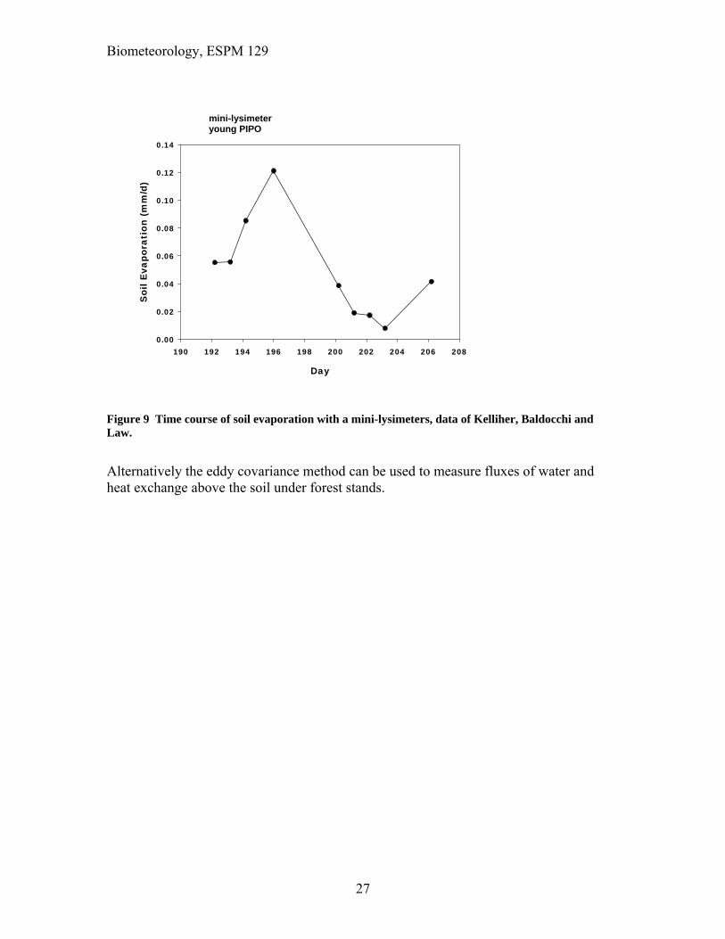
Figure 9 Time course of soil evaporation with a mini-lysimeters, data of Kelliher, Baldocchi and Law.

Alternatively the eddy covariance method can be used to measure fluxes of water and heat exchange above the soil under forest stands.

Day

190 192 194 196 198 200 202 204 206 208

Soi

l Eva

pora

tion

(m

m/d

)

0.00

0.02

0.04

0.06

0.08

0.10

0.12

0.14

mini-lysimeteryoung PIPO


28

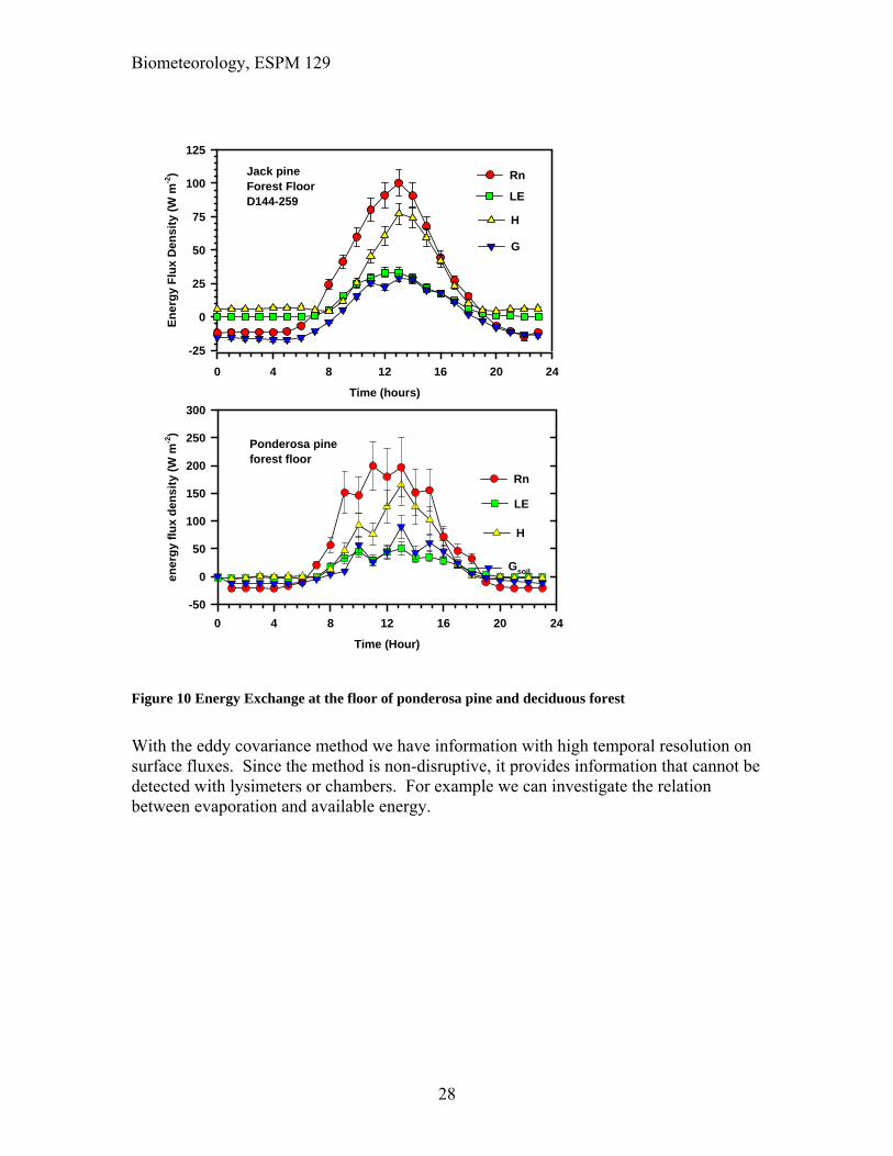
Figure 10 Energy Exchange at the floor of ponderosa pine and deciduous forest

With the eddy covariance method we have information with high temporal resolution on surface fluxes. Since the method is non-disruptive, it provides information that cannot be detected with lysimeters or chambers. For example we can investigate the relation between evaporation and available energy.

Ponderosa pineforest floor

Time (Hour)

0 4 8 12 16 20 24

en

erg

y fl

ux

den

sit

y (W

m-2

)

-50

0

50

100

150

200

250

300

LE

H

Rn

Gsoil

Jack pineForest FloorD144-259

Time (hours)

0 4 8 12 16 20 24

En

erg

y F

lux

Den

sity

(W

m-2

)

-25

0

25

50

75

100

125

Rn

LE

H

G


29

Figure 11 Non-linear response of forest floor evaporation as a function of available energy

Note that it saturates! Interactions between the time scale of equilibrium evaporation and the repeat time of coherent structures have been hypothesized to cause this effect (Baldocchi and Meyers, 1991). Modeling Soil Evaporation Soil evaporation models are key components of meteorological SVAT models, as well as climate, hydrology and biogeochemistry models. Mahfouf and Noilhan (1991) surveyed the literature and present algorithms for bare soil evaporation and have evaluated several algorithms. The most basic form is:

Soila

asg RR

qThqLLE

))((

h is the relative humidity at the site of evaporation, q is the mixing ratio, qs is the saturated mixing ratio at T, Ra is the soil boundary layer resistance and Rsoil is the soil resistance. Note that the end point of the moisture potential is not as simples as with a leaf, which we assume is saturated. We need to assess the relative humidity in soils, which is not one as the soil dries.

Rn -G: forest floor (W m-2)

-50 0 50 100 150 200

LE

fo

rest

flo

or

(W m

-2)

-10

0

10

20

30

40

50

60

70

ponderosa pine forest

jack pine forest temperate deciduousforest


30

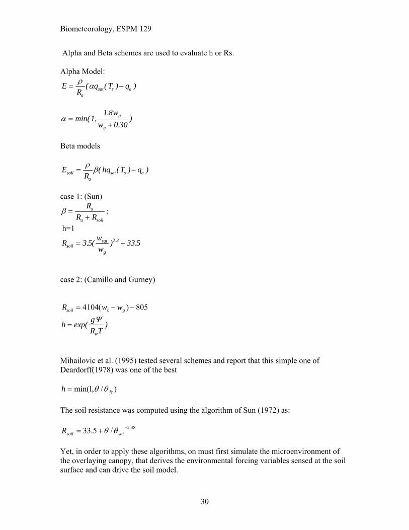
Alpha and Beta schemes are used to evaluate h or Rs. Alpha Model:

ER

q T qa

sat s a ( ( ) )

min( ,.

.)1

1 8

0 30

w

wg

g

Beta models

ER

hq T qsoila

sat s a ( ( ) )

case 1: (Sun)

R

R Ra

a soil

;

h=1

Rw

wsoilsat

g

3 5 33 52 3. ( ) ..

case 2: (Camillo and Gurney) R w wsoil s g 4104 805( )

hg

R Tw

exp( )

Mihailovic et al. (1995) tested several schemes and report that this simple one of Deardorff(1978) was one of the best

)/,1min( fch

The soil resistance was computed using the algorithm of Sun (1972) as:

38.2/5.33 satsoilR

Yet, in order to apply these algorithms, on must first simulate the microenvironment of the overlaying canopy, that derives the environmental forcing variables sensed at the soil surface and can drive the soil model.


31

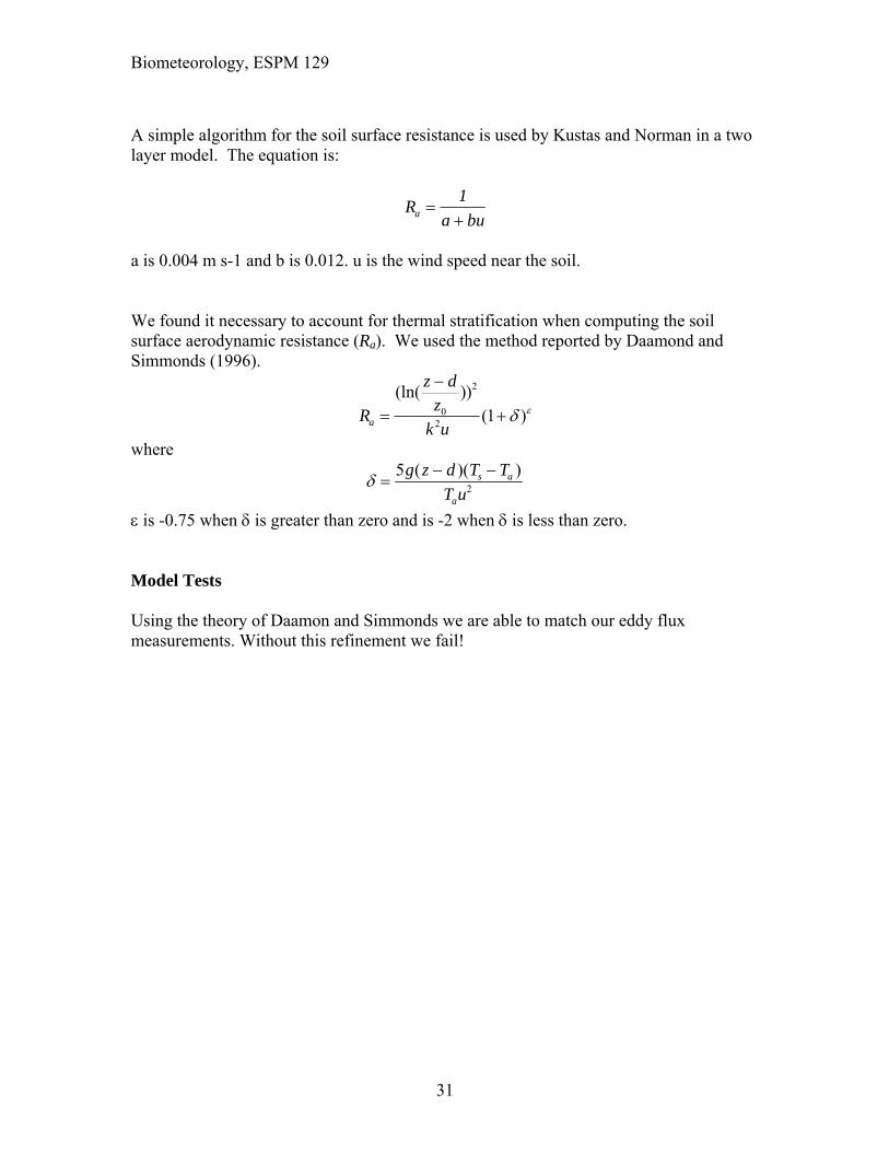
A simple algorithm for the soil surface resistance is used by Kustas and Norman in a two layer model. The equation is:

Ra bua

1

a is 0.004 m s-1 and b is 0.012. u is the wind speed near the soil.

We found it necessary to account for thermal stratification when computing the soil surface aerodynamic resistance (Ra). We used the method reported by Daamond and Simmonds (1996).

R

z dz

k ua

(ln( ))

( )0

2

2 1

where

5

2

g z d T T

T us a

a

( )( )

is -0.75 when is greater than zero and is -2 when is less than zero. Model Tests Using the theory of Daamon and Simmonds we are able to match our eddy flux measurements. Without this refinement we fail!


32

Figure 12 Measurements and calculations of energy exchange from the forest floor of a ponderosa pine with CANVEG. Mean diurnal patterns

Sensitivity Tests 1. Litter

Ponderosa PineForest FloorD187-205, 1996

Rn

et (

W m

-2)

-50

0

50

100

150

200

250

300

measured

calculated

LE

(W

m-2

)

-25

0

25

50

75

H (

W m

-2)

0

50

100

150

200

Time (hours)

0 4 8 12 16 20 24

G (

W m

-2)

-75-50-25

0255075

100125150


33

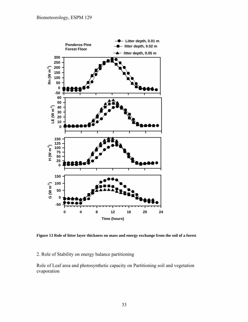
Figure 13 Role of litter layer thickness on mass and energy exchange from the soil of a forest

2. Role of Stability on energy balance partitioning Role of Leaf area and photosynthetic capacity on Partitioning soil and vegetation evaporation

Rn

(W

m-2

)

-500

50100150200250300

LE

(W

m-2

)

0102030405060

Litter depth, 0.01 mlitter depth, 0.02 m

H (

W m

-2)

0255075

100125150

Time (hours)

0 4 8 12 16 20 24

G (

W m

-2)

-50

0

50

100

150

Ponderos PineForest Floor

litter depth, 0.05 m


34

Figure 14 Fraction of soil evaporation to total canopy evaporation as leaf area index and photosynthetic capacity change. Soil evaporation can range from 5 to 20 % of total, assuming moist soil surface.

LAI * Vcmax

0 20 40 60 80 100 120 140 160 180 200

QE

,so

il/Q

E

0.00

0.05

0.10

0.15

0.20

0.25

0.30


35

Figure 15 Role of thermal stratification on heat and energy exchange at the floor of a forest. By ignoring thermal convection, the surface gets too hot and radiates away more long wave energy, thereby diminishing Rn.

Resources Soil Water Characteristics Hydraulic Properties Calculator http://www.bsyse.wsu.edu/saxton/soilwater/

Rn

(W

m-2

)

-500

50100150200250300

LE

(W

m-2

)

010203040506070

Ra=f(stability)

Ra: neutralH

(W

m-2

)

0255075

100125150

Time (hours)

0 4 8 12 16 20 24

G (

W m

-2)

-50

0

50

100

150

200

Ponderos PineForest Floor


36

Resources Global Texture and Water Holding Capacities http://www-eosdis.ornl.gov/SOILS/Webb.html References: Amundson et al. 1998. Geoderma. 82: 83-114. Baldocchi, D.D. and T.P. Meyers. 1991. Trace gas exchange at the floor of a deciduous

forest: I. evaporation and CO2 efflux. Journal Geophysical Research,

Atmospheres. 96: 7271-7285 Baldocchi, D.D., B.E. Law and P. Anthoni. 2000. On measuring and modeling energy

fluxes above the floor of a homogeneous and heterogeneous conifer forest. Agricultural and Forest Meteorology 102, 187-206.

Baver,L.D., Garnder. W.H. and Gardner, W.R. 1971. Soil Physics. Wiley and Sons. Campbell, G.S. 1985.Soil Physics with Basic: transport models for soil-plant systems.

Elsevier. Kabat, P., Hutjes, R. and Feddes, R.A. 1997. The scaling characteristics of soil

parameters: from plot scale heterogeneity to subgrid parameterization. Journal of Hydrology.

Kabat, P. and Beekma, J. Water in the unsaturated zone. In. Drainage Principles and

Application. Wageningen, The Netherlands. Pp. 383-434 Monteith, J.L. and M.H. Unsworth. 1990. Principles of Environmental Physics. E.A.

Arnold. Parlange, M., Hopmans JW (eds). 1999. Vadose Zone Hydrology Tindall, J.A. and J.R. Kunkel. 1999. Unsaturated Zone Hydrology for Scientists and

Engineers. Prentice Hall.624 pp. Tietje, O. and Tapkenhinrichs. 1993. Evaluation of Pedo-Transfer Functions. Soil

Science Soc. America. 57, 1088-1095. van Geunuchten. M. and D.R. Nielsen. 1985. On describing and predicting hydraulic

properties of unsaturated soils. Annales Geophysicae. 3, 615-628.


37

Campbell, G.S. and J.M. Norman 1998. An Introduction to Environmental Biophysics.

Springer Verlag, New York. 286 p. Clapp, R.B. and G.M. Hornberger 1978. Empirical Equations for Some Soil Hydraulic-

Properties. Water Resources Research. 14:601-604. Jenny, H. 1994. Factors of Soil Formation: A System of Quantitative Pedology. Dover

Press. Philip, J.R. 1995. Desperately Seeking Darcy in Dijon. Soil Sci Soc Am J. 59:319-324. Van Genuchten, M.T. 1980. A Closed-Form Equation for Predicting the Hydraulic

Conductivity of Unsaturated Soils. Soil Science Society of America Journal. 44:892-898.

van Genuchten, M.T. and E.A. Sudicky 1999. Recent advances in Vadose zone flow and transport modeling. In Vadose Zone Hydrology Eds. M. Parlange and J.W. Hopmans. Oxford Press, New York, pp. 155-193.

Lecture 35 Soil Physics, Moisture Transfer in Soils, …...Biometeorology, ESPM 129 1 Lecture 35...

Documents

Transcript of Lecture 35 Soil Physics, Moisture Transfer in Soils, …...Biometeorology, ESPM 129 1 Lecture 35...