
Lecture 23 Lidar sensing of gases, aerosols, and clouds
13
1 Lecture 23 Lidar sensing of gases, aerosols, and clouds 1. The lidar equation 2. Examples of lidar sensing of aerosols, gases, and clouds. 3. Lidars in space: LITE and CALIPSO Required reading: S: 8.4-8.5 Additional/advanced reading: Weitkamp: Chapter 1 CALIPSO: http://www-calipso.larc.nasa.gov/ CALIPSO Data User's Guide: http://www-calipso.larc.nasa.gov/resources/calipso_users_guide/ Browse Image Tutorial: http://www-calipso.larc.nasa.gov/resources/calipso_users_guide/browse/index.php Winker, D. M., and Coauthors, 2010: The CALIPSO Mission: A Global 3D View of Aerosols and Clouds. Bull. Amer. Meteor. Soc., 91, 1211–1229. Young, S. A., M. A. Vaughan, R. E. Kuehn, D. M. Winker, 2013: The Retrieval of Profiles of Particulate Extinction from Cloud–Aerosol Lidar and Infrared Pathfinder Satellite Observations (CALIPSO) Data: Uncertainty and Error Sensitivity Analyses. J. Atmos. Oceanic Technol., 30, 395–428
Transcript of Lecture 23 Lidar sensing of gases, aerosols, and clouds

1
Lecture 23
Lidar sensing of gases, aerosols, and clouds
1. The lidar equation
2. Examples of lidar sensing of aerosols, gases, and clouds.
3. Lidars in space: LITE and CALIPSO
Required reading:
S: 8.4-8.5
Additional/advanced reading:
Weitkamp: Chapter 1
CALIPSO: http://www-calipso.larc.nasa.gov/
CALIPSO Data User's Guide:
http://www-calipso.larc.nasa.gov/resources/calipso_users_guide/
Browse Image Tutorial:
http://www-calipso.larc.nasa.gov/resources/calipso_users_guide/browse/index.php
Winker, D. M., and Coauthors, 2010: The CALIPSO Mission: A Global 3D View of
Aerosols and Clouds. Bull. Amer. Meteor. Soc., 91, 1211–1229.
Young, S. A., M. A. Vaughan, R. E. Kuehn, D. M. Winker, 2013: The Retrieval of
Profiles of Particulate Extinction from Cloud–Aerosol Lidar and Infrared Pathfinder
Satellite Observations (CALIPSO) Data: Uncertainty and Error Sensitivity Analyses. J.
Atmos. Oceanic Technol., 30, 395–428

2
1. Lidar equation
In general, the form of a lidar equation depends upon the kind of interaction invoked by
the laser radiation.
Let’s consider elastic scattering. Similar to the derivation of the radar equation, the lidar
equation can be written as
))(2exp(42
)(2
rdrkkh
R
CRP e
R
o
br
[23.1]
where C is the lidar constant (includes Pt, receiver cross-section and other instrument
factors);
b/4 (in units of km-1sr-1) is called the backscattering factor or lidar backscattering
coefficient or backscattering coefficient;
e is the volume extinction coefficient; and tp is the lidar pulse duration (h=ctp)
Solutions of the lidar equation:
In general, both the volume extinction coefficiente and backscattering coefficientb
are unknown (see Eq.[23.1])
It is necessary to assume some kind of relation between e andb (called the
extinction-to-backscattering ratio)
EXAMPLE: Consider Rayleigh scattering. Assuming no absorption at the lidar
wavelength, the volume extinction coefficient is equal to the volume scattering
coefficient
se kk
On the other hand, Eq.[21.4] gives
)180( 0 Pkk sb
Using the Rayleigh scattering phase function, we have
5.1))180(cos1(4
3)180( 020 P

3
Thus, for Rayleigh scattering
essb kkPkk 5.15.1)180( [23.2]
To eliminate system constants, the range-corrected signal variable, S, can be defined as
))(ln()( 2 RPRRS r [23.3]
If So is the signal at the reference range R0, from Eq.[23.1] we have
drrkk
kRSRS e
R
Rob
b )(2ln)()(
0,
0
or in the differential form
)(2)(
)(
1Rk
dR
Rdk
RkdR
dSe
b
b
[23.4]
Solution of the lidar equation based on the slope method: assumes that the scatterers are
homogeneously distributed along the lidar path so
0)(
dR
Rdkb [23.5]
Thus
ekdR
dS2 [23.6]
and ke is estimated from the slope of the plot S vs. R
Limitations: applicable for a homogeneous path only.
Techniques based on the extinction-to-backscattering ratio:
use a priori relationship between ke and kb typically in the form
n
eb bkk [23.7]
where b and n are specified constants.
Substituting Eq.[23.7] in Eq.[23.4], we have
)(2)(
)(Rk
dR
Rdk
Rk
n
dR
dSe
e
e
[23.8]

4
with a general solution at the range R
drn
SS
nk
n
SS
kR
Re
e
o
0
0,
0
exp21
exp
[23.9]
NOTE:
Eq.[23.9] is derived ignoring the multiple scattering
Eq.[23.9] requires the assumption on the extinction-to-backscattering ratio
Eq.[23.9] is instable with respect to ke (some modifications were introduced to
avoid this problem. For instance, use the reference point at the predetermined end
range, Rm, so the solution is generated for R< Rm instead of R>Ro)
2. Examples of lidar sensing of aerosols , gases, and clouds.
Retrieval of the gas density from DIAL measurements:
DIfferential Absorption Lidar (DIAL) uses two wavelengths: one is in the maximum of
the absorption line of the gas of interest, and a second wavelength is in the region of low
absorption.
For each wavelength, the total extinction coefficient is due to the aerosol
extinction and the absorption by the gas (assumed that Rayleigh scattering is easy to
correct for)
gagaeree kkk ,, )()( [23.10]
where
aerek , is the aerosol volume extinction coefficient; g is the density of the absorbing gas;
and gak , is the mass absorption coefficient of the absorbing gas.
The two wavelengths are selected so that the aerosol optical properties are the same at
these wavelengths
)()( 2,1, aereaere kk and )()( 2,1, aerbaerb kk [23.11]
Taking the logarithm of both sites of Eq.[23.1], we have (for each wavelength)
5
rdrkkh
R
CPRP e
R
o
btr
)(2)42
ln()/)(ln(2
[23.12]
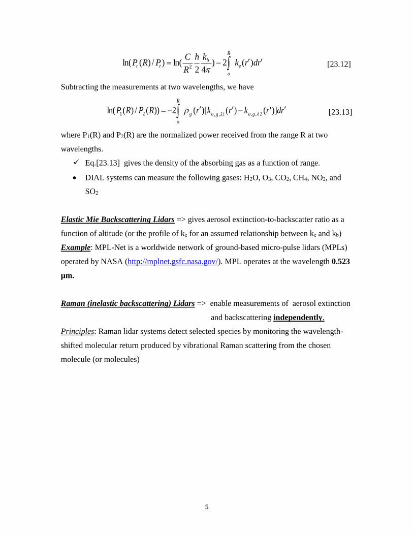
Subtracting the measurements at two wavelengths, we have
rdrkrkrRPRP gagag
R
o
)]'()()[(2))(/)(ln( 2,,1,,21 [23.13]
where P1(R) and P2(R) are the normalized power received from the range R at two
wavelengths.
Eq.[23.13] gives the density of the absorbing gas as a function of range.
DIAL systems can measure the following gases: H2O, O3, CO2, CH4, NO2, and
SO2
Elastic Mie Backscattering Lidars => gives aerosol extinction-to-backscatter ratio as a
function of altitude (or the profile of ke for an assumed relationship between ke and kb)
Example: MPL-Net is a worldwide network of ground-based micro-pulse lidars (MPLs)
operated by NASA (http://mplnet.gsfc.nasa.gov/). MPL operates at the wavelength 0.523
µm.
Raman (inelastic backscattering) Lidars => enable measurements of aerosol extinction
and backscattering independently.
Principles: Raman lidar systems detect selected species by monitoring the wavelength-
shifted molecular return produced by vibrational Raman scattering from the chosen
molecule (or molecules)
6
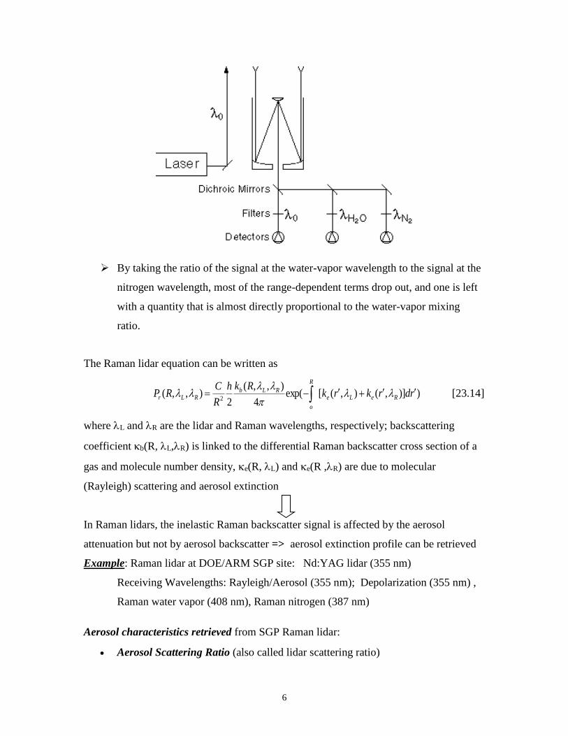
By taking the ratio of the signal at the water-vapor wavelength to the signal at the
nitrogen wavelength, most of the range-dependent terms drop out, and one is left
with a quantity that is almost directly proportional to the water-vapor mixing
ratio.
The Raman lidar equation can be written as
))],(),([exp(4
),,(
2),,(
2rdrkrk
Rkh
R
CRP ReLe
R
o
RLbRLr
[23.14]
where L and R are the lidar and Raman wavelengths, respectively; backscattering
coefficient b(R, L,R) is linked to the differential Raman backscatter cross section of a
gas and molecule number density, e(R, L) and e(R ,R) are due to molecular
(Rayleigh) scattering and aerosol extinction
In Raman lidars, the inelastic Raman backscatter signal is affected by the aerosol
attenuation but not by aerosol backscatter => aerosol extinction profile can be retrieved
Example: Raman lidar at DOE/ARM SGP site: Nd:YAG lidar (355 nm)
Receiving Wavelengths: Rayleigh/Aerosol (355 nm); Depolarization (355 nm) ,
Raman water vapor (408 nm), Raman nitrogen (387 nm)
Aerosol characteristics retrieved from SGP Raman lidar:
Aerosol Scattering Ratio (also called lidar scattering ratio)

7
is defined as the ratio of the total (aerosol+molecular) scattering to molecular scattering
[kb,m(,z)+ kb,a(,z))]/ kb,m(,z)
Aerosol Backscattering Coefficient
Profiles of the aerosol volume backscattering coefficient kb(=355 nm, z) are computed
using the aerosol scattering ratio profiles derived from the SGP Raman Lidar data and
profiles of the molecular backscattering coefficient. The molecular backscattering
coefficient is obtained from the molecular density profile which is computed using
radiosonde profiles of pressure and temperature from the balloon-borne sounding system
(BBSS) and/or the Atmospheric Emitted Radiance Interferometer (AERI). No additional
data and/or assumptions are required.
Aerosol Extinction/Backscatter Ratio
Profiles of the aerosol extinction/backscatter ratio are derived by dividing the aerosol
extinction profiles by the aerosol backscattering profiles.
Aerosol Optical Thickness
Aerosol optical thickness is derived by integrating the aerosol extinction profiles with
altitude.

8
Figure 23.1 Examples of retrievals using the Raman lidar.

9
CO2 lidar at 9.25 m and 10.6 m: measures the backscattering coefficient
Example: Jet Propulsion Lab (JPL) CO2 lidar (almost continuous operation since 1984):
vertical resolution is about 200 m throughout the troposphere and lower
stratosphere (up to about 30km)
Figure 23.2. Integrated backscatter from the free troposphere (upper panel) and the
lower stratosphere (lower panel) column above the JPL Pasadena site since the eruption
of the Philippine volcano Mt. Pinatubo in June of 1991 (Tratt et al.)
10
Lidar sensing of clouds.
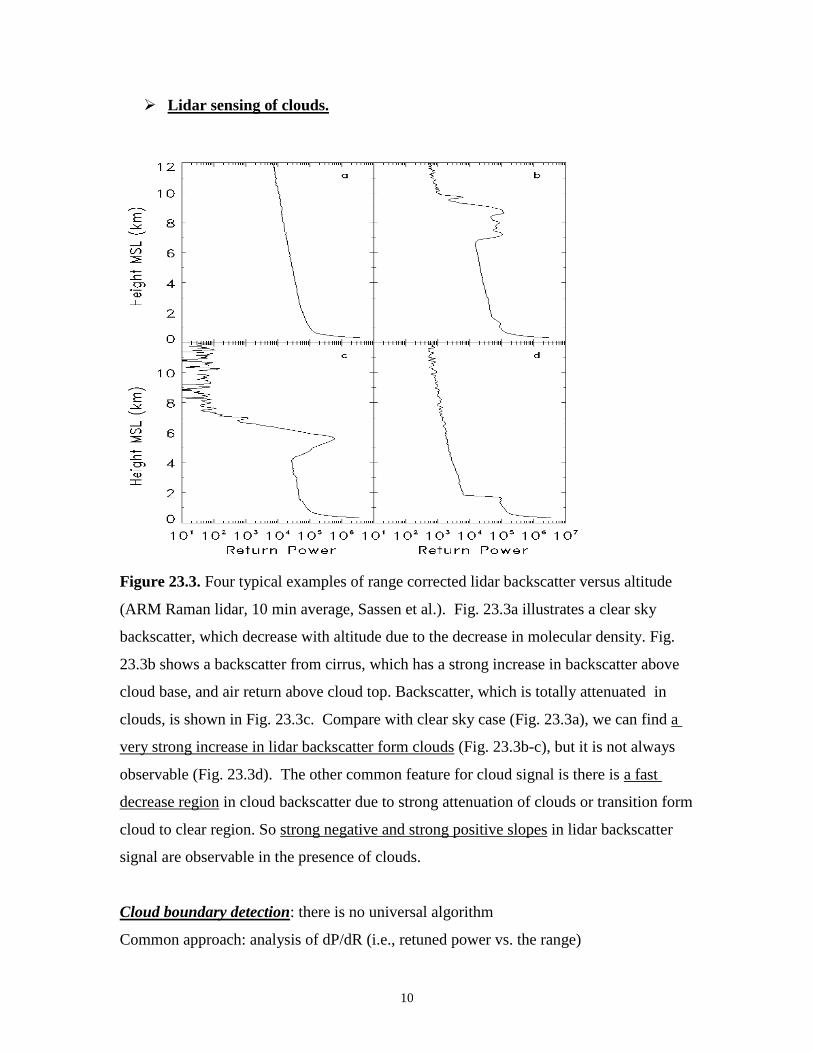
Figure 23.3. Four typical examples of range corrected lidar backscatter versus altitude
(ARM Raman lidar, 10 min average, Sassen et al.). Fig. 23.3a illustrates a clear sky
backscatter, which decrease with altitude due to the decrease in molecular density. Fig.
23.3b shows a backscatter from cirrus, which has a strong increase in backscatter above
cloud base, and air return above cloud top. Backscatter, which is totally attenuated in
clouds, is shown in Fig. 23.3c. Compare with clear sky case (Fig. 23.3a), we can find a
very strong increase in lidar backscatter form clouds (Fig. 23.3b-c), but it is not always
observable (Fig. 23.3d). The other common feature for cloud signal is there is a fast
decrease region in cloud backscatter due to strong attenuation of clouds or transition form
cloud to clear region. So strong negative and strong positive slopes in lidar backscatter
signal are observable in the presence of clouds.
Cloud boundary detection: there is no universal algorithm
Common approach: analysis of dP/dR (i.e., retuned power vs. the range)

11
3. Lidars in space: LITE and CALIPSO
LITE (Lidar In-space Technology Experiment) (http://www-lite.larc.nasa.gov/)
LITE flew on Discovery in September 1994
LITE was operated for 53 hours, resulting in over 40 GBytes of data covering
1.4 million kilometers of ground track;
YAG lasers which emit simultaneously at the three harmonically related
wavelengths of 1064 nm (infrared), 532 nm (visible green), and 355 nm
(ultraviolet). The two-laser system provides redundancy in case one laser fails.
Only one laser operates at a time.
LITE provided the first highly detailed global view of the vertical structure of clouds and
aerosols
CALIPSO (Cloud-Aerosol Lidar and Infrared Pathfinder Satellite Observations)
satellite has been launched in April 2006 (http://www-calipso.larc.nasa.gov/)
CALIPSO has three instruments: Cloud-Aerosol Lidar with Orthogonal Polarization
(CALIOP); Three-channel Imaging Infrared Radiometer (IIR); Wide Field Camera
(WFC)
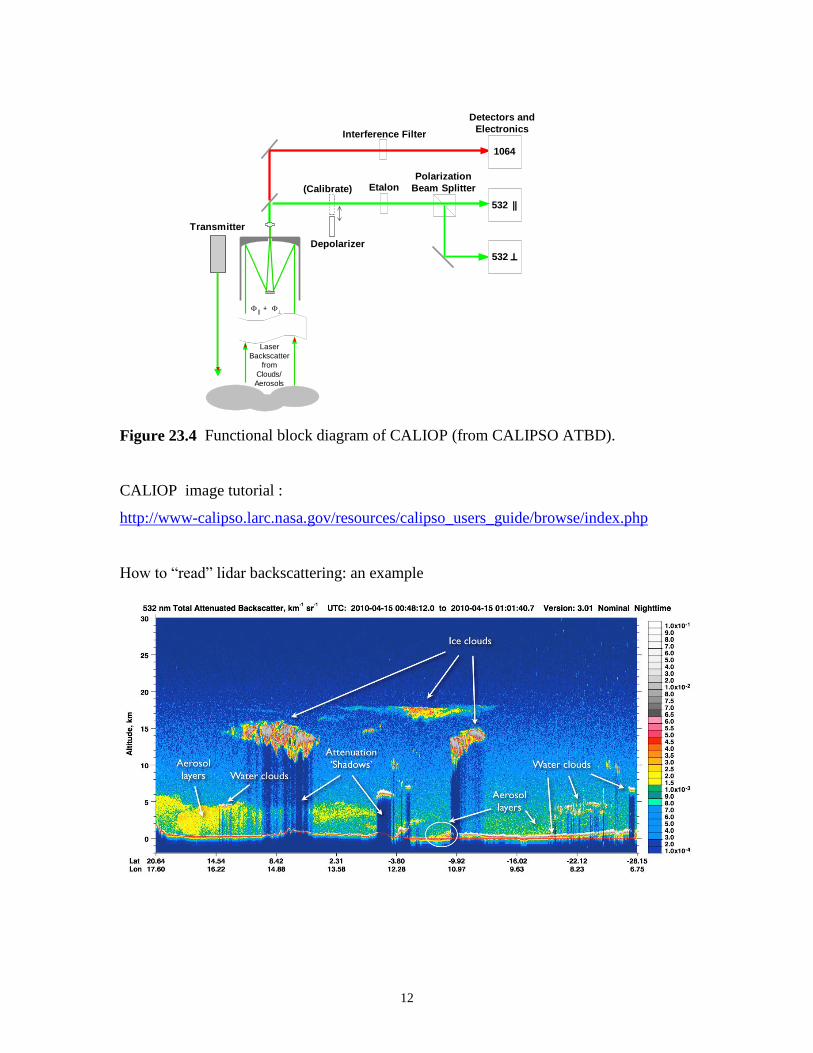
CALIOP is a two-wavelength (532 nm and 1064 nm) polarization-sensitive lidar that
provides high-resolution vertical profiles of aerosols and clouds. It has three receiver
channels: one measuring the 1064-nm backscattered intensity, and two channels
measuring orthogonally polarized components (parallel and perpendicular to the
polarization plane of the transmitted beam) of the 532-nm backscattered signal. It has a
footprint at the Earth's surface (from a 705-km orbit) of about 90 meters and vertical
resolution of 30 meters.
12
Figure 23.4 Functional block diagram of CALIOP (from CALIPSO ATBD).
CALIOP image tutorial :
http://www-calipso.larc.nasa.gov/resources/calipso_users_guide/browse/index.php
How to “read” lidar backscattering: an example
Etalon
532
Polarization
Beam Splitter
|| +
1064
532
Interference Filter
Laser
Backscatter
from
Clouds/
Aerosols
Detectors and
Electronics
Depolarizer
(Calibrate)
Transmitter
13
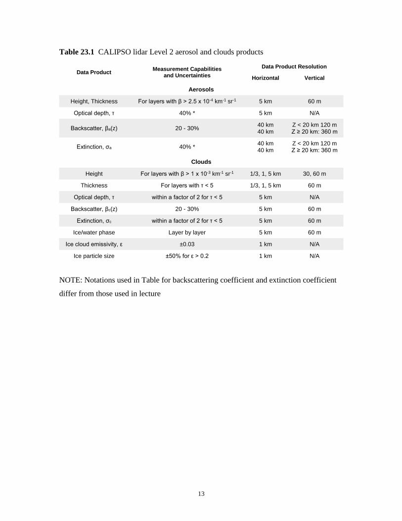
Table 23.1 CALIPSO lidar Level 2 aerosol and clouds products
Data Product Measurement Capabilities
and Uncertainties
Data Product Resolution
Horizontal Vertical
Aerosols
Height, Thickness For layers with β > 2.5 x 10⁻⁴ km-1 sr-1 5 km 60 m
Optical depth, τ 40% * 5 km N/A
Backscatter, βa(z) 20 - 30% 40 km 40 km
Z < 20 km 120 m Z ≥ 20 km: 360 m
Extinction, σa 40% * 40 km 40 km
Z < 20 km 120 m Z ≥ 20 km: 360 m
Clouds
Height For layers with β > 1 x 10⁻³ km-1 sr-1 1/3, 1, 5 km 30, 60 m
Thickness For layers with τ < 5 1/3, 1, 5 km 60 m
Optical depth, τ within a factor of 2 for τ < 5 5 km N/A
Backscatter, βc(z) 20 - 30% 5 km 60 m
Extinction, σc within a factor of 2 for τ < 5 5 km 60 m
Ice/water phase Layer by layer 5 km 60 m
Ice cloud emissivity, ε ±0.03 1 km N/A
Ice particle size ±50% for ε > 0.2 1 km N/A
NOTE: Notations used in Table for backscattering coefficient and extinction coefficient
differ from those used in lecture


