Lecture 2: Probability and Random...
34
Lecture 2: Probability and Random Variables Department of Electrical Engineering Princeton University September 18, 2013 ELE 525: Random Processes in Information Systems Hisashi Kobayashi Textbook: Hisashi Kobayashi, Brian L. Mark and William Turin, Probability, Random Processes and Statistical Analysis (Cambridge University Press, 2012) 9/18/2013 1 Copyright Hisashi Kobayashi 2013
Transcript of Lecture 2: Probability and Random...
Lecture 2:Probability and Random Variables
Department of Electrical EngineeringPrinceton UniversitySeptember 18, 2013
ELE 525: Random Processes in Information Systems
Hisashi Kobayashi
Textbook: Hisashi Kobayashi, Brian L. Mark and William Turin, Probability, Random Processes and Statistical Analysis (Cambridge University Press, 2012)
9/18/2013 1Copyright Hisashi Kobayashi 2013
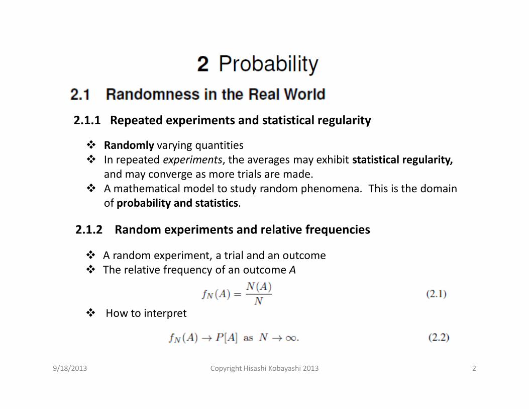
Randomly varying quantities In repeated experiments, the averages may exhibit statistical regularity,
and may converge as more trials are made. A mathematical model to study random phenomena. This is the domain
of probability and statistics.
29/18/2013 Copyright Hisashi Kobayashi 2013
2.1.1 Repeated experiments and statistical regularity
2.1.2 Random experiments and relative frequencies
A random experiment, a trial and an outcome The relative frequency of an outcome A
How to interpret

2.1.2 Random experiments and relative frequencies-cont’d
3
Construct an abstract model of probabilities such that the probabilities behave like the limits of the relative frequencies.
The law of large numbers.
9/18/2013 Copyright Hisashi Kobayashi 2013
Note: Axiomatic method in mathematics: The oldest and most famous example of axioms is Euclid’s axioms in geometry. In his book entitled Elements , Euclid (aka Euclid of Alexandria 330BC?-375BC?) deduced all propositions (or theorems) of what is now called Euclidean geometry from the following five axioms (or sometimes called postulates).
Axiom 1: We can draw a straight line segment joining any two points.Axiom 2: We can extend any straight line segment indefinitely in a straight
line.Axiom 3: We can draw a circle with any point as its center and any distance
as its radius.
9/18/2013 Copyright Hisashi Kobayashi 2013 4
Axiom 4: Are all right angles are congruent (i.e., equal to each other)Axiom 5: If two straight lines intersect a third straight line in such a way that the sum of the inner angles on one side is less than two right angles, then the two lines inevitably must intersect each other on that side if extended indefinitely (known as the parallel postulate).
Many mathematicians attempted to deduce Axiom 5 from Axioms 1-4, but failed. Around 1823-1831, the Hungarian mathematician János Bolyai(1802-1860) and the Russian mathematician Nicolai Labachevsky (1792-1856) independently discovered a non-Euclidean geometry , now known as hyperbolic geometry, based entirely on Axioms 1-4.
Carl Friedrich Gauss (1777-1855) had also discovered the existence of non-Euclidean geometry by around 1824, but did not publish his theory for fear of getting involved in a philosophical dispute concerning the notion of space and time held by the German philosopher Immanuel Kant (1724=1804).
Kant states that: “Space is not an empirical concept which has been derived from outer experiences.” On the contrary: “…it is the subjective condition of sensibility, under which alone outer intuition is possible for us.”
2.1.2 Random experiments and relative frequencies-cont’d
5
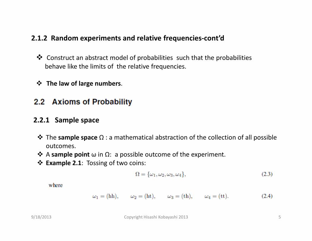
Construct an abstract model of probabilities such that the probabilities behave like the limits of the relative frequencies.
The law of large numbers.
9/18/2013 Copyright Hisashi Kobayashi 2013
2.2.1 Sample space
The sample space Ω : a mathematical abstraction of the collection of all possible outcomes.
A sample point ω in Ω: a possible outcome of the experiment. Example 2.1: Tossing of two coins:
2.2.2 Event
6
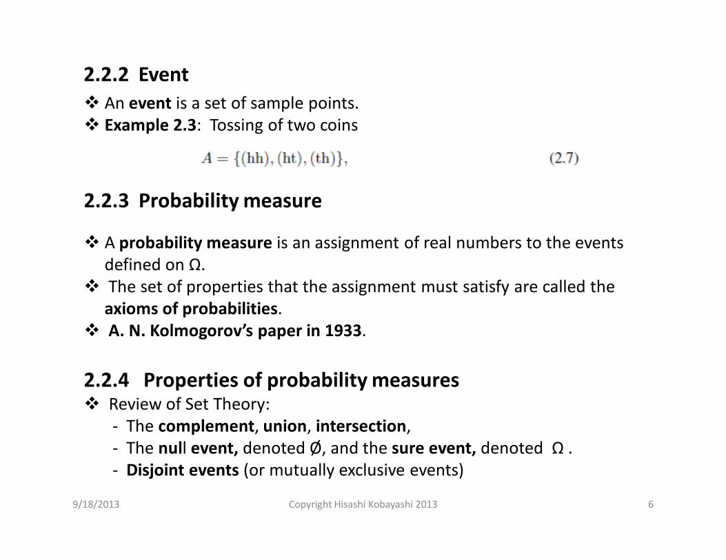
An event is a set of sample points. Example 2.3: Tossing of two coins
2.2.3 Probability measure
A probability measure is an assignment of real numbers to the events defined on Ω.
The set of properties that the assignment must satisfy are called the axioms of probabilities.
A. N. Kolmogorov’s paper in 1933.
9/18/2013 Copyright Hisashi Kobayashi 2013
2.2.4 Properties of probability measures Review of Set Theory:
- The complement, union, intersection,- The null event, denoted Ø, and the sure event, denoted Ω . - Disjoint events (or mutually exclusive events)
7
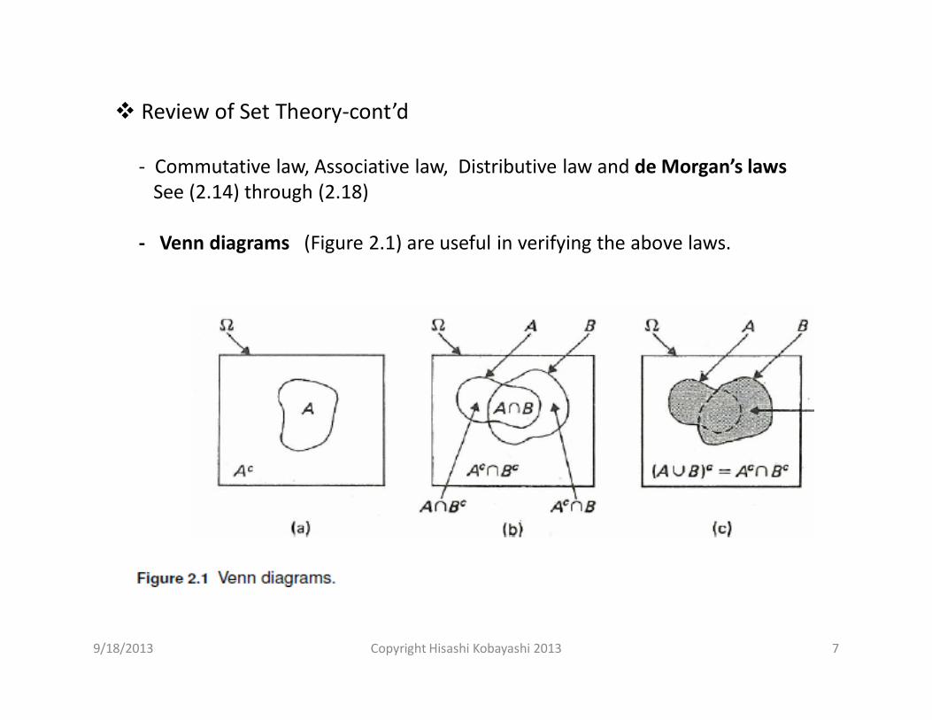
Review of Set Theory-cont’d
- Commutative law, Associative law, Distributive law and de Morgan’s lawsSee (2.14) through (2.18)
- Venn diagrams (Figure 2.1) are useful in verifying the above laws.
9/18/2013 Copyright Hisashi Kobayashi 2013
8
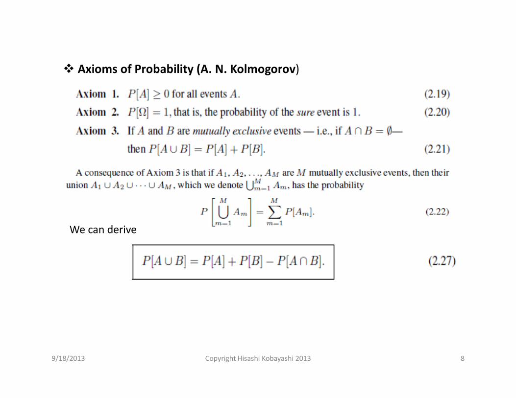
Axioms of Probability (A. N. Kolmogorov)
9/18/2013 Copyright Hisashi Kobayashi 2013
We can derive

9
We must extend Axiom 3 to deal with infinitely many events:
9/18/2013 Copyright Hisashi Kobayashi 2013
Because of Axiom 4, we require that the collection of events be closed under countable unions:
109/18/2013 Copyright Hisashi Kobayashi 2013
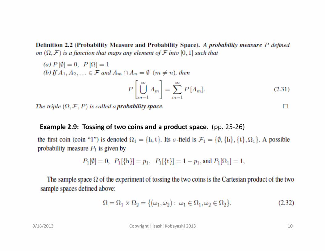
Example 2.9: Tossing of two coins and a product space. (pp. 25-26)
119/18/2013 Copyright Hisashi Kobayashi 2013
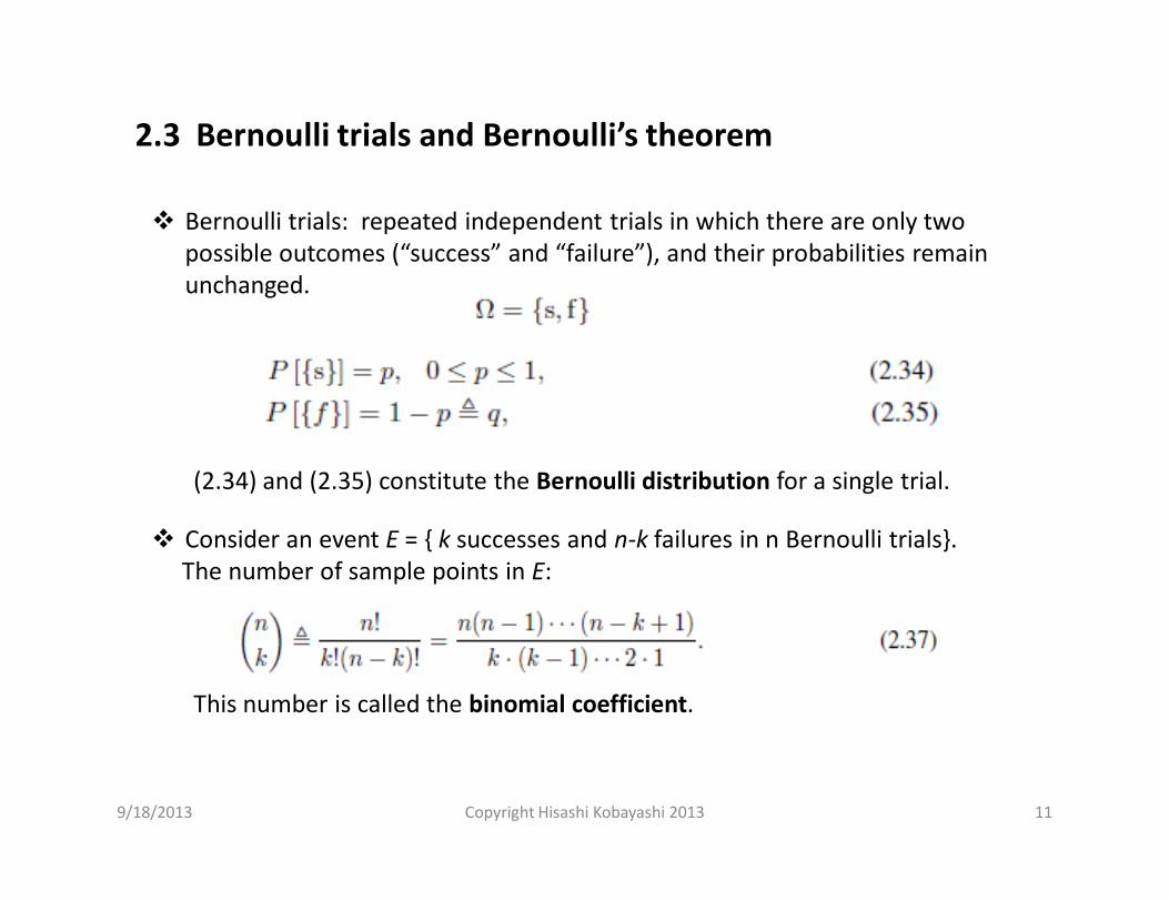
2.3 Bernoulli trials and Bernoulli’s theorem
Bernoulli trials: repeated independent trials in which there are only two possible outcomes (“success” and “failure”), and their probabilities remain unchanged.
(2.34) and (2.35) constitute the Bernoulli distribution for a single trial.
Consider an event E = { k successes and n-k failures in n Bernoulli trials}.The number of sample points in E:
This number is called the binomial coefficient.
129/18/2013 Copyright Hisashi Kobayashi 2013
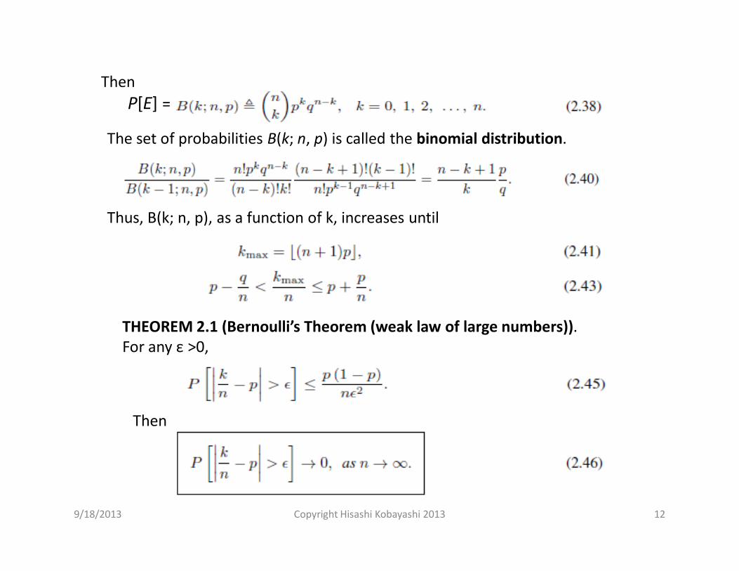
ThenP[E] =
The set of probabilities B(k; n, p) is called the binomial distribution.
Thus, B(k; n, p), as a function of k, increases until
THEOREM 2.1 (Bernoulli’s Theorem (weak law of large numbers)).For any ε >0,
Then
139/18/2013 Copyright Hisashi Kobayashi 2013
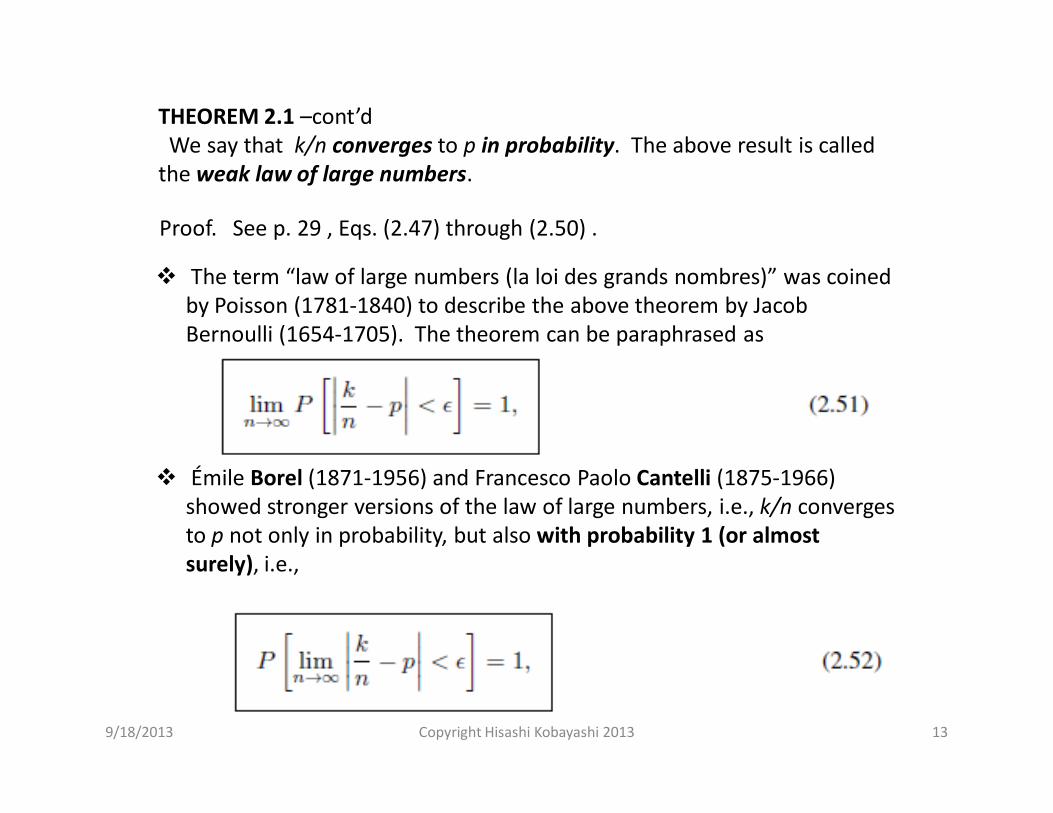
THEOREM 2.1 –cont’dWe say that k/n converges to p in probability. The above result is called
the weak law of large numbers.
Proof. See p. 29 , Eqs. (2.47) through (2.50) .
The term “law of large numbers (la loi des grands nombres)” was coined by Poisson (1781-1840) to describe the above theorem by Jacob Bernoulli (1654-1705). The theorem can be paraphrased as
Émile Borel (1871-1956) and Francesco Paolo Cantelli (1875-1966) showed stronger versions of the law of large numbers, i.e., k/n converges to p not only in probability, but also with probability 1 (or almost surely), i.e.,

9/18/2013 Copyright Hisashi Kobayashi 2013 14
A simpler proof of the weak law of large numbers (WLLN) see p. 250 . The difference between the WLLN and the strong law of large numbers (SLLN) is
equivalent to that between convergence in probability and almost sure convergence . (see pp. 280-288).
Further discussions of the WLLN and SLLN, see Sections 11.3.2 and 11.3.3.
159/18/2013 Copyright Hisashi Kobayashi 2013
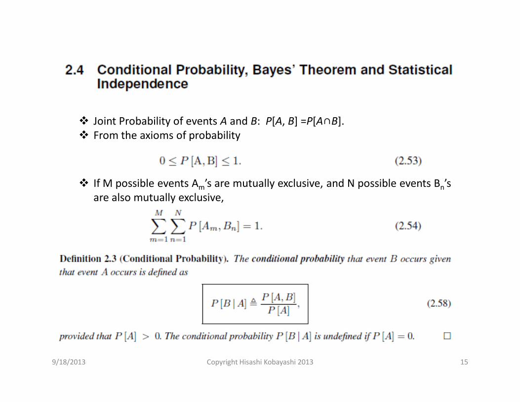
Joint Probability of events A and B: P[A, B] =P[A∩B]. From the axioms of probability
If M possible events Am’s are mutually exclusive, and N possible events Bn’sare also mutually exclusive,
169/18/2013 Copyright Hisashi Kobayashi 2013
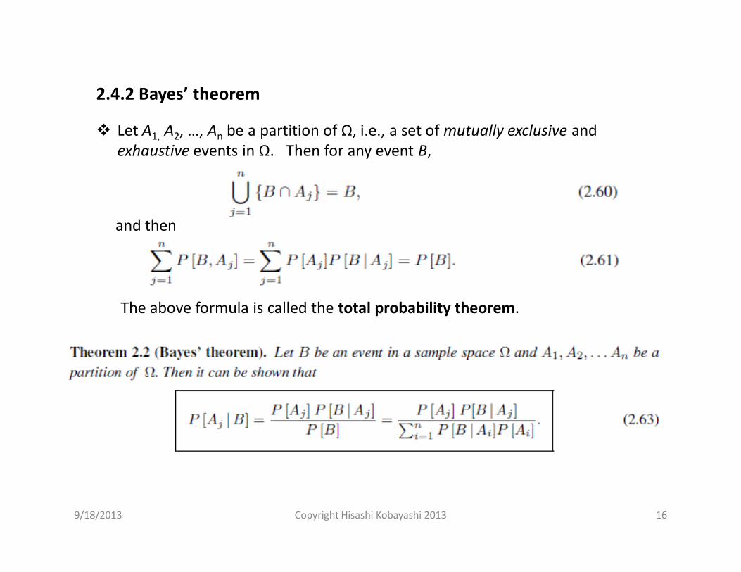
2.4.2 Bayes’ theorem
Let A1, A2, …, An be a partition of Ω, i.e., a set of mutually exclusive and exhaustive events in Ω. Then for any event B,
and then
The above formula is called the total probability theorem.

9/18/2013 Copyright Hisashi Kobayashi 2013 17
Answer: Let
Then
9/18/2013 Copyright Hisashi Kobayashi 2013 18
Frequentist probabilities and Baysian probabilities
Frequentists’ view: probabilities can be assigned only to outcomes of an experiment that can be repeated many times.
Bayesians’ view: the notion of probability is applicable to any situation or event to which we attach some uncertainty or belief.
The Bayesian view is appealing to those who investigate probabilistic learning theory.
The Bayes’ theorem provides fundamental principles of learning based on data or evidence.
You may find the following article of interest and helpful.“Are you a Bayeisan or a Frequentist? (Or Bayesian Statistics 101)” in
Panos Ipeirotis’s bloghttp://www.behind-the-enemy-lines.com/2008/01/are-you-bayesian-or-
frequentist-or.html See also “Section 4.5 Bayesian inference and conjugate priors” (pp. 97-
102”) of the textbook on this subject.

9/18/2013 Copyright Hisashi Kobayashi 2013 19
2.4.3 Statistical Independence of Events
9/18/2013 Copyright Hisashi Kobayashi 2013 20
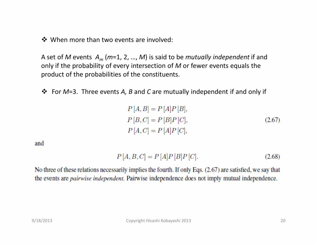
When more than two events are involved:
A set of M events Am (m=1, 2, …, M) is said to be mutually independent if and only if the probability of every intersection of M or fewer events equals the product of the probabilities of the constituents.
For M=3. Three events A, B and C are mutually independent if and only if
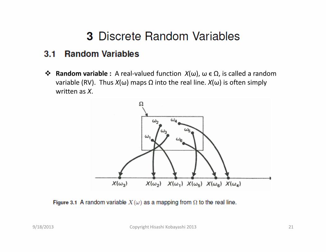
Random variable : A real-valued function X(ω), ω ϵ Ω, is called a random variable (RV). Thus X(ω) maps Ω into the real line. X(ω) is often simply written as X.
219/18/2013 Copyright Hisashi Kobayashi 2013

3.1.1 Distribution function
229/18/2013 Copyright Hisashi Kobayashi 2013
239/18/2013 Copyright Hisashi Kobayashi 2013
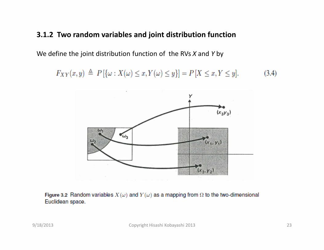
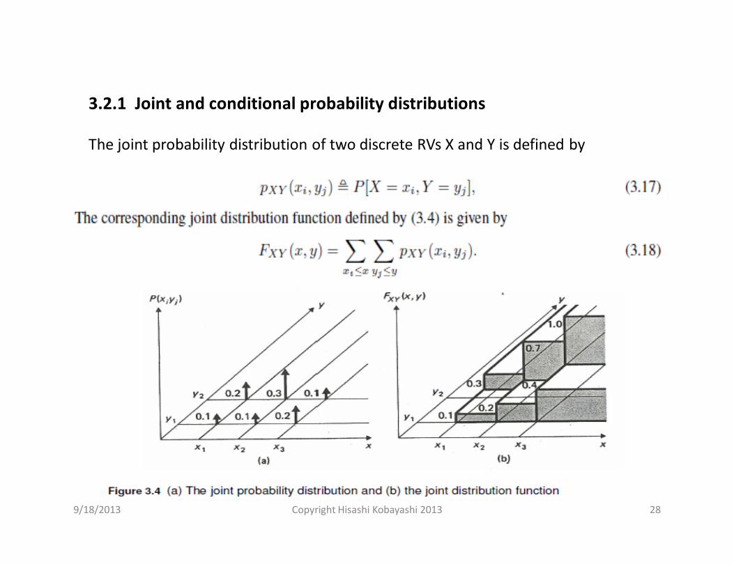
3.1.2 Two random variables and joint distribution function
We define the joint distribution function of the RVs X and Y by
249/18/2013 Copyright Hisashi Kobayashi 2013
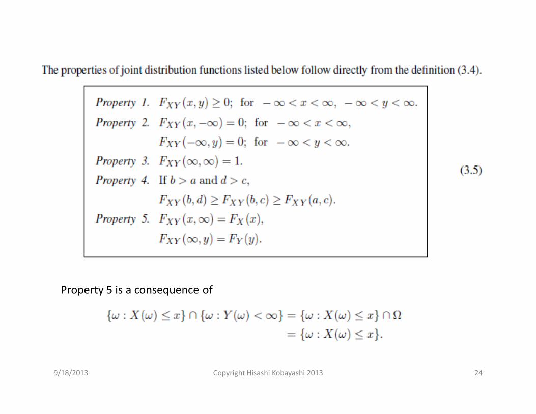
Property 5 is a consequence of
259/18/2013 Copyright Hisashi Kobayashi 2013
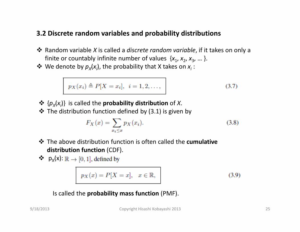
3.2 Discrete random variables and probability distributions
Random variable X is called a discrete random variable, if it takes on only a finite or countably infinite number of values {x1, x2, x3, … }.
We denote by pX(xi), the probability that X takes on xi :
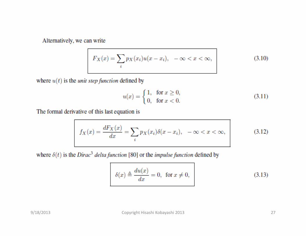
{pX(xi)} is called the probability distribution of X. The distribution function defined by (3.1) is given by
The above distribution function is often called the cumulative distribution function (CDF).
pX(x):
Is called the probability mass function (PMF).

269/18/2013 Copyright Hisashi Kobayashi 2013
279/18/2013 Copyright Hisashi Kobayashi 2013
289/18/2013 Copyright Hisashi Kobayashi 2013
3.2.1 Joint and conditional probability distributions
The joint probability distribution of two discrete RVs X and Y is defined by
299/18/2013 Copyright Hisashi Kobayashi 2013
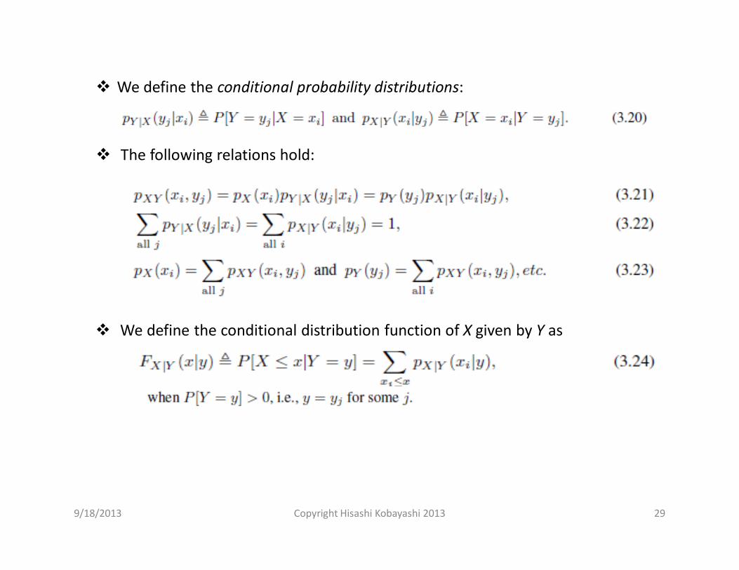
We define the conditional probability distributions:
The following relations hold:
We define the conditional distribution function of X given by Y as
9/18/2013 Copyright Hisashi Kobayashi 2013 30
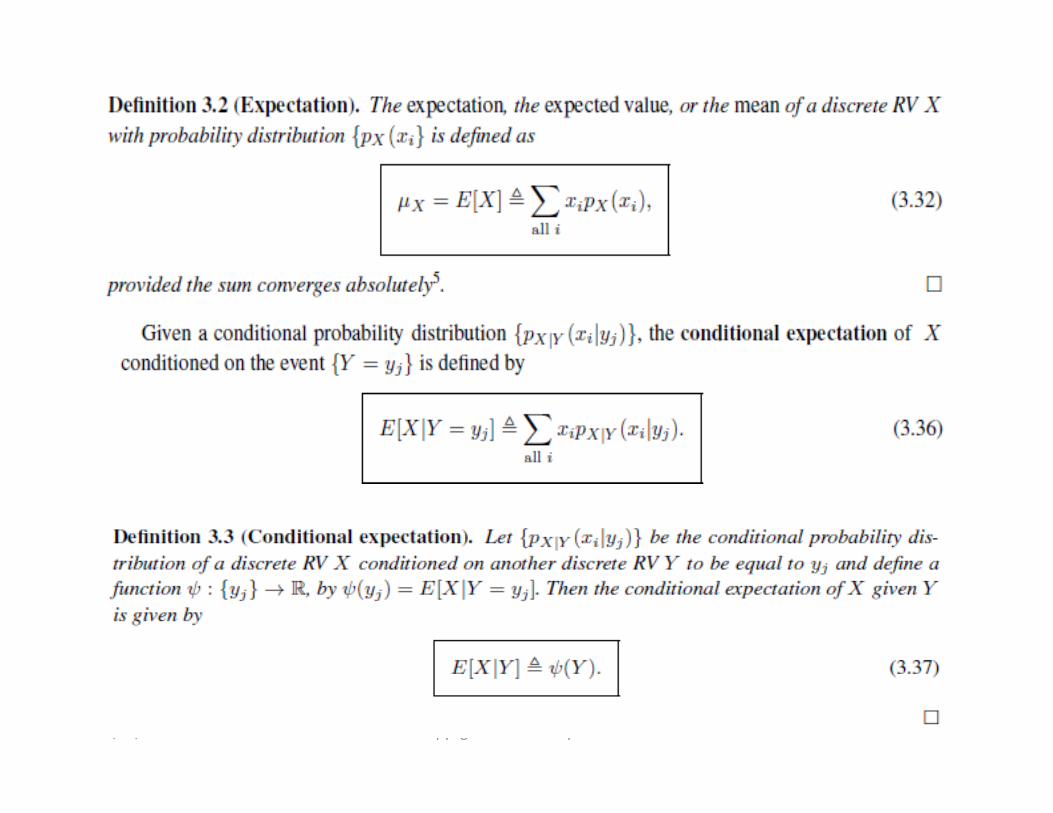
9/18/2013 Copyright Hisashi Kobayashi 2013 31
9/18/2013 Copyright Hisashi Kobayashi 2013 32
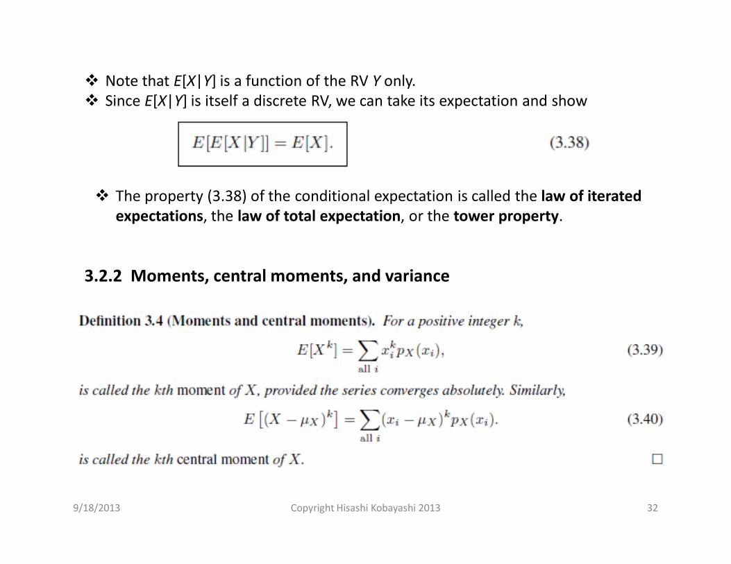
Note that E[X|Y] is a function of the RV Y only. Since E[X|Y] is itself a discrete RV, we can take its expectation and show
The property (3.38) of the conditional expectation is called the law of iterated expectations, the law of total expectation, or the tower property.
3.2.2 Moments, central moments, and variance
9/18/2013 Copyright Hisashi Kobayashi 2013 33
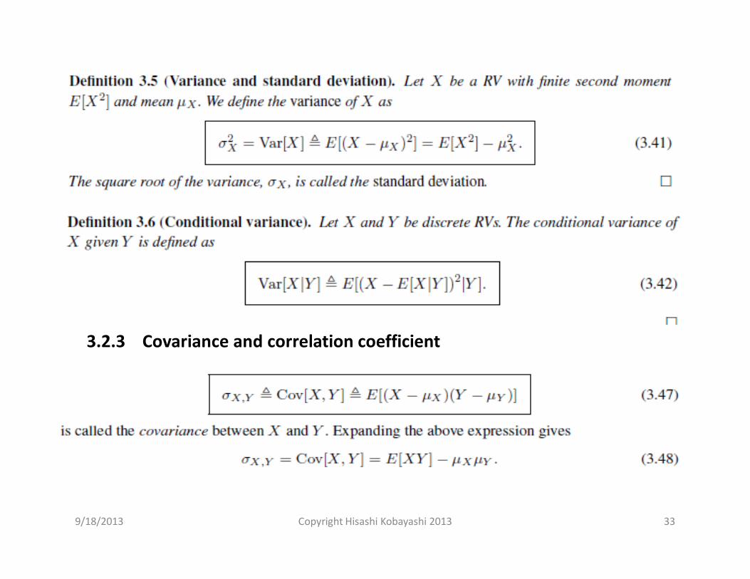
3.2.3 Covariance and correlation coefficient
9/18/2013 Copyright Hisashi Kobayashi 2013 34
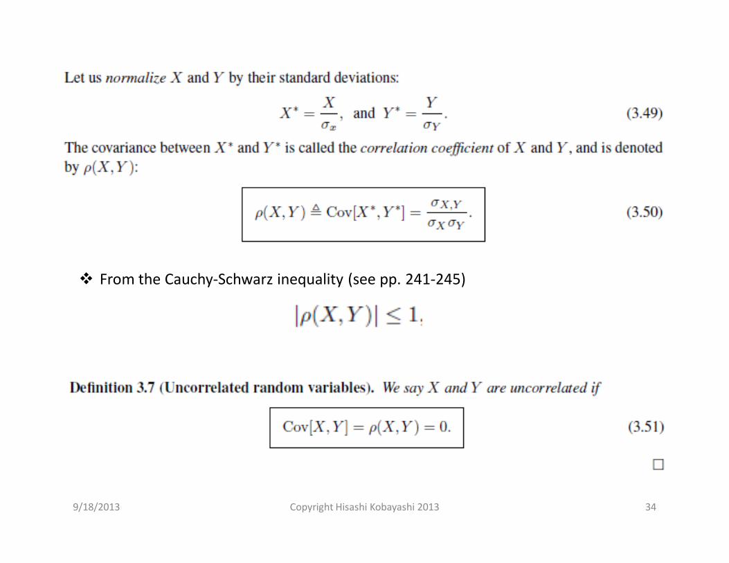
From the Cauchy-Schwarz inequality (see pp. 241-245)