Lecture 18 - Fitting CAR and SAR Models
43
Lecture 18 Fitting CAR and SAR Models Colin Rundel 3/29/2018 1
Transcript of Lecture 18 - Fitting CAR and SAR Models

Lecture 18Fitting CAR and SAR Models
Colin Rundel3/29/2018
1

Fitting areal models
2
CAR vs SAR
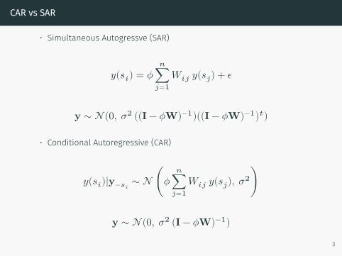
• Simultaneous Autogressve (SAR)
𝑦(𝑠𝑖) = 𝜙𝑛
∑𝑗=1
𝑊𝑖𝑗 𝑦(𝑠𝑗) + 𝜖
𝐲 ∼ 𝒩(0, 𝜎2 ((𝐈 − 𝜙𝐖)−1)((𝐈 − 𝜙𝐖)−1)𝑡)
• Conditional Autoregressive (CAR)
𝑦(𝑠𝑖)|𝐲−𝑠𝑖∼ 𝒩 (𝜙
𝑛∑𝑗=1
𝑊𝑖𝑗 𝑦(𝑠𝑗), 𝜎2)
𝐲 ∼ 𝒩(0, 𝜎2 (𝐈 − 𝜙𝐖)−1)
3

Some generalizations
Generally speaking we will want to work with a scaled / normalized versionof the weight matrix,
𝑊𝑖𝑗𝑊𝑖⋅
When 𝑊 is an adjacency matrix we can express this as
𝐃−1𝐖
where 𝐃−1 = diag(1/|𝑁(𝑠𝑖)|).We can also allow 𝜎2 to vary between locations, we can define this as𝐃𝜏 = diag(1/𝜎2
𝑖 ) and most often we use
𝐃−1𝜎 = diag( 𝜎2
|𝑁(𝑠𝑖)|) = 𝜎2𝐃−1.
4

Revised SAR Model
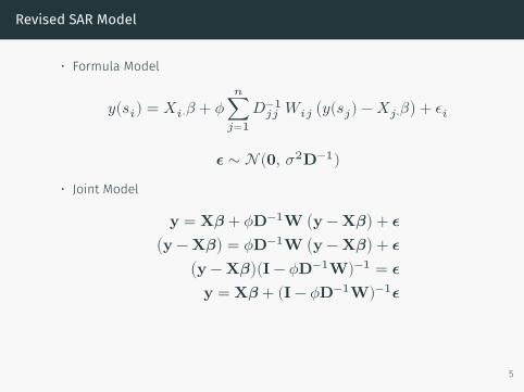
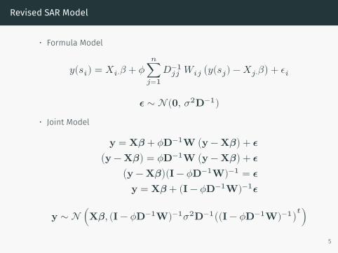
• Formula Model
𝑦(𝑠𝑖) = 𝑋𝑖⋅𝛽 + 𝜙𝑛
∑𝑗=1
𝐷−1𝑗𝑗 𝑊𝑖𝑗 (𝑦(𝑠𝑗) − 𝑋𝑗⋅𝛽) + 𝜖𝑖
𝝐 ∼ 𝒩(𝟎, 𝜎2𝐃−1)• Joint Model
𝐲 = 𝐗𝜷 + 𝜙𝐃−1𝐖 (𝐲 − 𝐗𝜷) + 𝝐(𝐲 − 𝐗𝜷) = 𝜙𝐃−1𝐖 (𝐲 − 𝐗𝜷) + 𝝐
(𝐲 − 𝐗𝜷)(𝐈 − 𝜙𝐃−1𝐖)−1 = 𝝐𝐲 = 𝐗𝜷 + (𝐈 − 𝜙𝐃−1𝐖)−1𝝐
𝐲 ∼ 𝒩 (𝐗𝜷, (𝐈 − 𝜙𝐃−1𝐖)−1𝜎2𝐃−1((𝐈 − 𝜙𝐃−1𝐖)−1)𝑡)
5
Revised SAR Model
• Formula Model
𝑦(𝑠𝑖) = 𝑋𝑖⋅𝛽 + 𝜙𝑛
∑𝑗=1
𝐷−1𝑗𝑗 𝑊𝑖𝑗 (𝑦(𝑠𝑗) − 𝑋𝑗⋅𝛽) + 𝜖𝑖
𝝐 ∼ 𝒩(𝟎, 𝜎2𝐃−1)• Joint Model
𝐲 = 𝐗𝜷 + 𝜙𝐃−1𝐖 (𝐲 − 𝐗𝜷) + 𝝐(𝐲 − 𝐗𝜷) = 𝜙𝐃−1𝐖 (𝐲 − 𝐗𝜷) + 𝝐
(𝐲 − 𝐗𝜷)(𝐈 − 𝜙𝐃−1𝐖)−1 = 𝝐𝐲 = 𝐗𝜷 + (𝐈 − 𝜙𝐃−1𝐖)−1𝝐
𝐲 ∼ 𝒩 (𝐗𝜷, (𝐈 − 𝜙𝐃−1𝐖)−1𝜎2𝐃−1((𝐈 − 𝜙𝐃−1𝐖)−1)𝑡)
5
Revised SAR Model
• Formula Model
𝑦(𝑠𝑖) = 𝑋𝑖⋅𝛽 + 𝜙𝑛
∑𝑗=1
𝐷−1𝑗𝑗 𝑊𝑖𝑗 (𝑦(𝑠𝑗) − 𝑋𝑗⋅𝛽) + 𝜖𝑖
𝝐 ∼ 𝒩(𝟎, 𝜎2𝐃−1)• Joint Model
𝐲 = 𝐗𝜷 + 𝜙𝐃−1𝐖 (𝐲 − 𝐗𝜷) + 𝝐(𝐲 − 𝐗𝜷) = 𝜙𝐃−1𝐖 (𝐲 − 𝐗𝜷) + 𝝐
(𝐲 − 𝐗𝜷)(𝐈 − 𝜙𝐃−1𝐖)−1 = 𝝐𝐲 = 𝐗𝜷 + (𝐈 − 𝜙𝐃−1𝐖)−1𝝐
𝐲 ∼ 𝒩 (𝐗𝜷, (𝐈 − 𝜙𝐃−1𝐖)−1𝜎2𝐃−1((𝐈 − 𝜙𝐃−1𝐖)−1)𝑡)
5

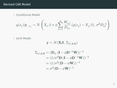
Revised CAR Model
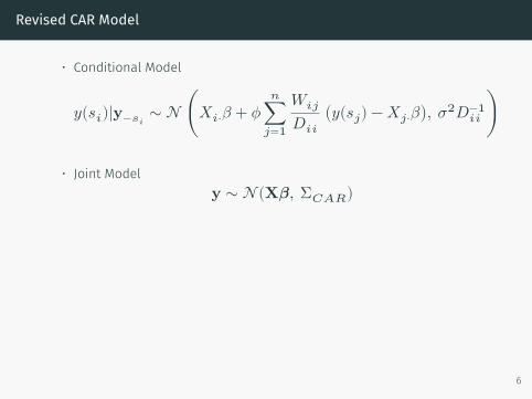
• Conditional Model
𝑦(𝑠𝑖)|𝐲−𝑠𝑖∼ 𝒩 (𝑋𝑖⋅𝛽 + 𝜙
𝑛∑𝑗=1
𝑊𝑖𝑗𝐷𝑖𝑖
(𝑦(𝑠𝑗) − 𝑋𝑗⋅𝛽), 𝜎2𝐷−1𝑖𝑖 )
• Joint Model
𝐲 ∼ 𝒩(𝐗𝜷, Σ𝐶𝐴𝑅)
Σ𝐶𝐴𝑅 = (𝐃𝜎 (𝐈 − 𝜙𝐃−1𝐖))−1
= (1/𝜎2𝐃 (𝐈 − 𝜙𝐃−1𝐖))−1
= (1/𝜎2(𝐃 − 𝜙𝐖))−1
= 𝜎2(𝐃 − 𝜙𝐖)−1
6
Revised CAR Model
• Conditional Model
𝑦(𝑠𝑖)|𝐲−𝑠𝑖∼ 𝒩 (𝑋𝑖⋅𝛽 + 𝜙
𝑛∑𝑗=1
𝑊𝑖𝑗𝐷𝑖𝑖
(𝑦(𝑠𝑗) − 𝑋𝑗⋅𝛽), 𝜎2𝐷−1𝑖𝑖 )
• Joint Model𝐲 ∼ 𝒩(𝐗𝜷, Σ𝐶𝐴𝑅)
Σ𝐶𝐴𝑅 = (𝐃𝜎 (𝐈 − 𝜙𝐃−1𝐖))−1
= (1/𝜎2𝐃 (𝐈 − 𝜙𝐃−1𝐖))−1
= (1/𝜎2(𝐃 − 𝜙𝐖))−1
= 𝜎2(𝐃 − 𝜙𝐖)−1
6
Revised CAR Model
• Conditional Model
𝑦(𝑠𝑖)|𝐲−𝑠𝑖∼ 𝒩 (𝑋𝑖⋅𝛽 + 𝜙
𝑛∑𝑗=1
𝑊𝑖𝑗𝐷𝑖𝑖
(𝑦(𝑠𝑗) − 𝑋𝑗⋅𝛽), 𝜎2𝐷−1𝑖𝑖 )
• Joint Model𝐲 ∼ 𝒩(𝐗𝜷, Σ𝐶𝐴𝑅)
Σ𝐶𝐴𝑅 = (𝐃𝜎 (𝐈 − 𝜙𝐃−1𝐖))−1
= (1/𝜎2𝐃 (𝐈 − 𝜙𝐃−1𝐖))−1
= (1/𝜎2(𝐃 − 𝜙𝐖))−1
= 𝜎2(𝐃 − 𝜙𝐖)−1
6
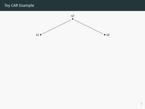
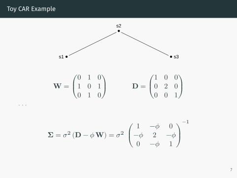
Toy CAR Example
s1
s2
s3
𝐖 = ⎛⎜⎝
0 1 01 0 10 1 0
⎞⎟⎠
𝐃 = ⎛⎜⎝
1 0 00 2 00 0 1
⎞⎟⎠
. . .
𝚺 = 𝜎2 (𝐃 − 𝜙 𝐖) = 𝜎2 ⎛⎜⎝
1 −𝜙 0−𝜙 2 −𝜙0 −𝜙 1
⎞⎟⎠
−1
7
Toy CAR Example
s1
s2
s3
𝐖 = ⎛⎜⎝
0 1 01 0 10 1 0
⎞⎟⎠
𝐃 = ⎛⎜⎝
1 0 00 2 00 0 1
⎞⎟⎠
. . .
𝚺 = 𝜎2 (𝐃 − 𝜙 𝐖) = 𝜎2 ⎛⎜⎝
1 −𝜙 0−𝜙 2 −𝜙0 −𝜙 1
⎞⎟⎠
−1
7

When does Σ exist?
check_sigma = function(phi) {Sigma_inv = matrix(c(1,-phi,0,-phi,2,-phi,0,-phi,1), ncol=3, byrow=TRUE)solve(Sigma_inv)
}
check_sigma(phi=0)## [,1] [,2] [,3]## [1,] 1 0.0 0## [2,] 0 0.5 0## [3,] 0 0.0 1
check_sigma(phi=0.5)## [,1] [,2] [,3]## [1,] 1.1666667 0.3333333 0.1666667## [2,] 0.3333333 0.6666667 0.3333333## [3,] 0.1666667 0.3333333 1.1666667
check_sigma(phi=-0.6)## [,1] [,2] [,3]## [1,] 1.28125 -0.46875 0.28125## [2,] -0.46875 0.78125 -0.46875## [3,] 0.28125 -0.46875 1.28125
8
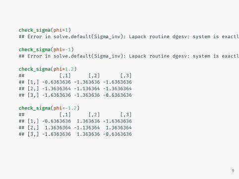
check_sigma(phi=1)## Error in solve.default(Sigma_inv): Lapack routine dgesv: system is exactly singular: U[3,3] = 0
check_sigma(phi=-1)## Error in solve.default(Sigma_inv): Lapack routine dgesv: system is exactly singular: U[3,3] = 0
check_sigma(phi=1.2)## [,1] [,2] [,3]## [1,] -0.6363636 -1.363636 -1.6363636## [2,] -1.3636364 -1.136364 -1.3636364## [3,] -1.6363636 -1.363636 -0.6363636
check_sigma(phi=-1.2)## [,1] [,2] [,3]## [1,] -0.6363636 1.363636 -1.6363636## [2,] 1.3636364 -1.136364 1.3636364## [3,] -1.6363636 1.363636 -0.6363636
9
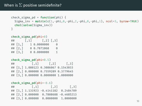
When is Σ positive semidefinite?
check_sigma_pd = function(phi) {Sigma_inv = matrix(c(1,-phi,0,-phi,2,-phi,0,-phi,1), ncol=3, byrow=TRUE)chol(solve(Sigma_inv))
}
check_sigma_pd(phi=0)## [,1] [,2] [,3]## [1,] 1 0.0000000 0## [2,] 0 0.7071068 0## [3,] 0 0.0000000 1
check_sigma_pd(phi=0.5)## [,1] [,2] [,3]## [1,] 1.080123 0.3086067 0.1543033## [2,] 0.000000 0.7559289 0.3779645## [3,] 0.000000 0.0000000 1.0000000
check_sigma_pd(phi=-0.6)## [,1] [,2] [,3]## [1,] 1.131923 -0.4141182 0.2484709## [2,] 0.000000 0.7808688 -0.4685213## [3,] 0.000000 0.0000000 1.0000000
10
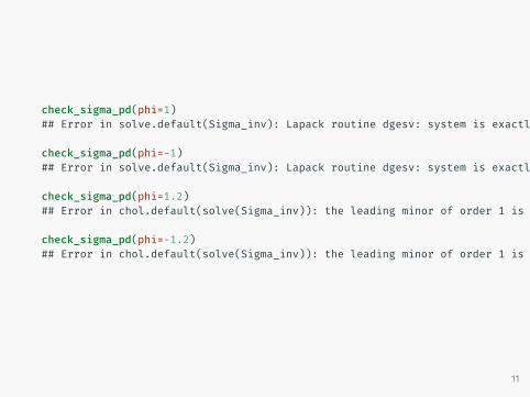
check_sigma_pd(phi=1)## Error in solve.default(Sigma_inv): Lapack routine dgesv: system is exactly singular: U[3,3] = 0
check_sigma_pd(phi=-1)## Error in solve.default(Sigma_inv): Lapack routine dgesv: system is exactly singular: U[3,3] = 0
check_sigma_pd(phi=1.2)## Error in chol.default(solve(Sigma_inv)): the leading minor of order 1 is not positive definite
check_sigma_pd(phi=-1.2)## Error in chol.default(solve(Sigma_inv)): the leading minor of order 1 is not positive definite
11
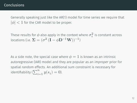
Conclusions
Generally speaking just like the AR(1) model for time series we require that|𝜙| < 1 for the CAR model to be proper.
These results for 𝜙 also apply in the context where 𝜎2𝑖 is constant across
locations (i.e. 𝚺 = (𝜎2 (𝐈 − 𝜙𝐃−1𝐖))−1)
As a side note, the special case where 𝜙 = 1 is known as an intrinsicautoregressive (IAR) model and they are popular as an improper prior forspatial random effects. An additional sum constraint is necessary foridentifiability (∑𝑛
𝑖=1 𝑦(𝑠𝑖) = 0).
12

Example - NC SIDS
34°N
34.5°N
35°N
35.5°N
36°N
36.5°N
84°W 82°W 80°W 78°W 76°W
34°N
34.5°N
35°N
35.5°N
36°N
36.5°N
84°W 82°W 80°W 78°W 76°W
5000
10000
15000
20000
BIR74
0
10
20
30
40
SID74
13
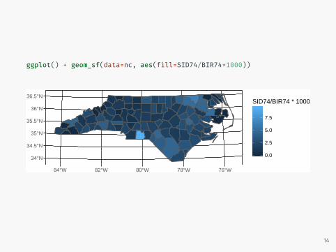
ggplot() + geom_sf(data=nc, aes(fill=SID74/BIR74*1000))
34°N
34.5°N
35°N
35.5°N
36°N
36.5°N
84°W 82°W 80°W 78°W 76°W
0.0
2.5
5.0
7.5
SID74/BIR74 * 1000
14

Using spautolm from spdep
library(spdep)
W = st_touches(nc, sparse=FALSE)listW = mat2listw(W)
listW## Characteristics of weights list object:## Neighbour list object:## Number of regions: 100## Number of nonzero links: 490## Percentage nonzero weights: 4.9## Average number of links: 4.9#### Weights style: M## Weights constants summary:## n nn S0 S1 S2## M 100 10000 490 980 10696
15

nc_coords = nc %>% st_centroid() %>% st_coordinates()
plot(st_geometry(nc))plot(listW, nc_coords, add=TRUE, col=”blue”, pch=16)
16

Moran’s I
spdep::moran.test(nc$SID74, listW)#### Moran I test under randomisation#### data: nc$SID74## weights: listW#### Moran I statistic standard deviate = 2.1707, p-value = 0.01498## alternative hypothesis: greater## sample estimates:## Moran I statistic Expectation Variance## 0.119089049 -0.010101010 0.003542176spdep::moran.test(1000*nc$SID74/nc$BIR74, listW)#### Moran I test under randomisation#### data: 1000 * nc$SID74/nc$BIR74## weights: listW#### Moran I statistic standard deviate = 3.6355, p-value = 0.0001387## alternative hypothesis: greater## sample estimates:## Moran I statistic Expectation Variance## 0.210046454 -0.010101010 0.003666802
17

Geary’s C
spdep::geary.test(nc$SID74, listW)#### Geary C test under randomisation#### data: nc$SID74## weights: listW#### Geary C statistic standard deviate = 0.91949, p-value = 0.1789## alternative hypothesis: Expectation greater than statistic## sample estimates:## Geary C statistic Expectation Variance## 0.88988684 1.00000000 0.01434105spdep::geary.test(nc$SID74/nc$BIR74, listW)#### Geary C test under randomisation#### data: nc$SID74/nc$BIR74## weights: listW#### Geary C statistic standard deviate = 3.0989, p-value = 0.0009711## alternative hypothesis: Expectation greater than statistic## sample estimates:## Geary C statistic Expectation Variance## 0.67796679 1.00000000 0.01079878
18
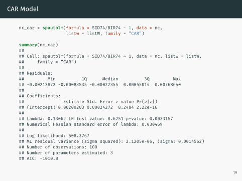
CAR Model
nc_car = spautolm(formula = SID74/BIR74 ~ 1, data = nc,listw = listW, family = ”CAR”)
summary(nc_car)#### Call: spautolm(formula = SID74/BIR74 ~ 1, data = nc, listw = listW,## family = ”CAR”)#### Residuals:## Min 1Q Median 3Q Max## -0.00213872 -0.00083535 -0.00022355 0.00055014 0.00768640#### Coefficients:## Estimate Std. Error z value Pr(>|z|)## (Intercept) 0.00200203 0.00024272 8.2484 2.22e-16#### Lambda: 0.13062 LR test value: 8.6251 p-value: 0.0033157## Numerical Hessian standard error of lambda: 0.030469#### Log likelihood: 508.3767## ML residual variance (sigma squared): 2.1205e-06, (sigma: 0.0014562)## Number of observations: 100## Number of parameters estimated: 3## AIC: -1010.8
19
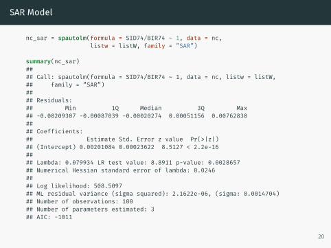
SAR Model
nc_sar = spautolm(formula = SID74/BIR74 ~ 1, data = nc,listw = listW, family = ”SAR”)
summary(nc_sar)#### Call: spautolm(formula = SID74/BIR74 ~ 1, data = nc, listw = listW,## family = ”SAR”)#### Residuals:## Min 1Q Median 3Q Max## -0.00209307 -0.00087039 -0.00020274 0.00051156 0.00762830#### Coefficients:## Estimate Std. Error z value Pr(>|z|)## (Intercept) 0.00201084 0.00023622 8.5127 < 2.2e-16#### Lambda: 0.079934 LR test value: 8.8911 p-value: 0.0028657## Numerical Hessian standard error of lambda: 0.0246#### Log likelihood: 508.5097## ML residual variance (sigma squared): 2.1622e-06, (sigma: 0.0014704)## Number of observations: 100## Number of parameters estimated: 3## AIC: -1011
20
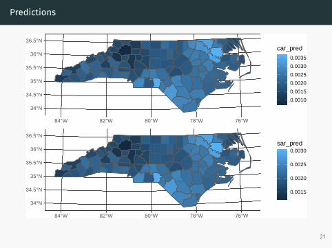
Predictions
34°N
34.5°N
35°N
35.5°N
36°N
36.5°N
84°W 82°W 80°W 78°W 76°W
34°N
34.5°N
35°N
35.5°N
36°N
36.5°N
84°W 82°W 80°W 78°W 76°W
0.0010
0.0015
0.0020
0.0025
0.0030
0.0035
car_pred
0.0015
0.0020
0.0025
0.0030sar_pred
21

Residuals
34°N
34.5°N
35°N
35.5°N
36°N
36.5°N
84°W 82°W 80°W 78°W 76°W
34°N
34.5°N
35°N
35.5°N
36°N
36.5°N
84°W 82°W 80°W 78°W 76°W
0.0000
0.0025
0.0050
0.0075car_resid
0.0000
0.0025
0.0050
0.0075sar_resid
22
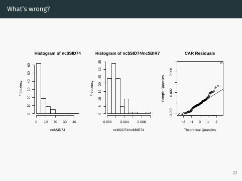
What’s wrong?
Histogram of nc$SID74
nc$SID74
Fre
quen
cy
0 10 20 30 40
010
2030
4050
60
Histogram of nc$SID74/nc$BIR74
nc$SID74/nc$BIR74
Fre
quen
cy
0.000 0.004 0.008
05
1015
2025
3035
−2 −1 0 1 2
−0.
002
0.00
20.
006
CAR Residuals
Theoretical Quantiles
Sam
ple
Qua
ntile
s
23
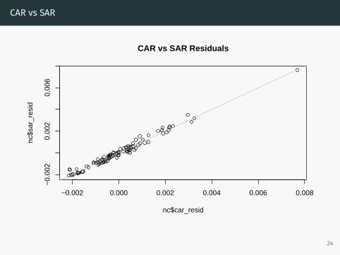
CAR vs SAR
−0.002 0.000 0.002 0.004 0.006 0.008
−0.
002
0.00
20.
006
CAR vs SAR Residuals
nc$car_resid
nc$s
ar_r
esid
24

Stan CAR Model
car_model = ”data {int<lower=0> N;vector[N] y;matrix[N,N] W;matrix[N,N] D;
}parameters {vector[N] w_s;real beta;real<lower=0> sigma2;real<lower=0> sigma2_w;real<lower=0,upper=1> phi;
}transformed parameters {vector[N] y_pred = beta + w_s;
}model {matrix[N,N] Sigma_inv = (D - phi * W) / sigma2;
w_s ~ multi_normal_prec(rep_vector(0,N), Sigma_inv);
beta ~ normal(0,10);sigma2 ~ cauchy(0,5);sigma2_w ~ cauchy(0,5);
y ~ normal(beta+w_s, sigma2_w);}”
25

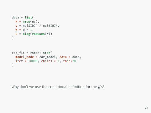
data = list(N = nrow(nc),y = nc$SID74 / nc$BIR74,W = W * 1,D = diag(rowSums(W))
)
car_fit = rstan::stan(model_code = car_model, data = data,iter = 10000, chains = 1, thin=20
)
Why don’t we use the conditional definition for the 𝑦’s?
26
data = list(N = nrow(nc),y = nc$SID74 / nc$BIR74,W = W * 1,D = diag(rowSums(W))
)
car_fit = rstan::stan(model_code = car_model, data = data,iter = 10000, chains = 1, thin=20
)
Why don’t we use the conditional definition for the 𝑦’s?
26
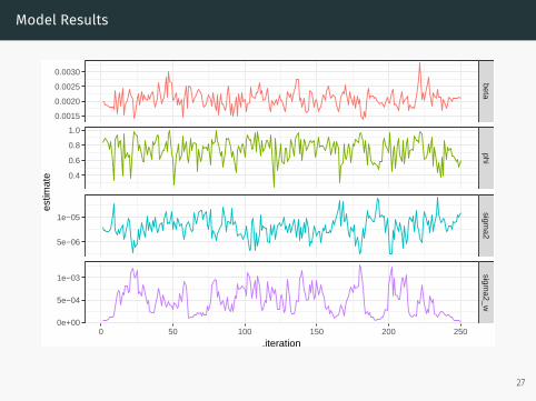
Model Results
betaphi
sigma2
sigma2_w
0 50 100 150 200 250
0.0015
0.0020
0.0025
0.0030
0.4
0.6
0.8
1.0
5e−06
1e−05
0e+00
5e−04
1e−03
.iteration
estim
ate
27

Predictions
28
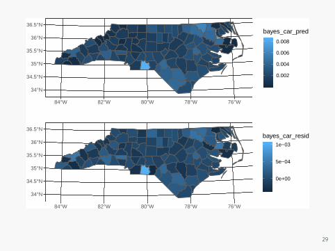
34°N
34.5°N
35°N
35.5°N
36°N
36.5°N
84°W 82°W 80°W 78°W 76°W
34°N
34.5°N
35°N
35.5°N
36°N
36.5°N
84°W 82°W 80°W 78°W 76°W
0.002
0.004
0.006
0.008
bayes_car_pred
0e+00
5e−04
1e−03
bayes_car_resid
29
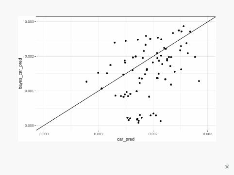
0.000
0.001
0.002
0.003
0.000 0.001 0.002 0.003
car_pred
baye
s_ca
r_pr
ed
30

Brief Aside - SAR Precision Matrix
Σ𝑆𝐴𝑅 = (𝐈 − 𝜙𝐃−1 𝐖)−1𝜎2 𝐃−1 ((𝐈 − 𝜙𝐃−1 𝐖)−1)𝑡
Σ−1𝑆𝐴𝑅 = ((𝐈 − 𝜙𝐃−1 𝐖)−1𝜎2 𝐃−1 ((𝐈 − 𝜙𝐃−1 𝐖)−1)𝑡)
−1
= (((𝐈 − 𝜙𝐃−1 𝐖)−1)𝑡)−1 1
𝜎2 𝐃 (𝐈 − 𝜙𝐃−1 𝐖)
= 1𝜎2 (𝐈 − 𝜙𝐃−1 𝐖)𝑡 𝐃 (𝐈 − 𝜙𝐃−1 𝐖)
31

Jags SAR Model
sar_model = ”data {
int<lower=0> N;vector[N] y;matrix[N,N] W_tilde;matrix[N,N] D;
}transformed data {
matrix[N,N] I = diag_matrix(rep_vector(1, N));}parameters {
vector[N] w_s;real beta;real<lower=0> sigma2;real<lower=0> sigma2_w;real<lower=0,upper=1> phi;
}transformed parameters {
vector[N] y_pred = beta + w_s;}model {
matrix[N,N] C = I - phi * W_tilde;matrix[N,N] Sigma_inv = C' * D * C / sigma2;
w_s ~ multi_normal_prec(rep_vector(0,N), Sigma_inv);
beta ~ normal(0,10);sigma2 ~ cauchy(0,5);sigma2_w ~ cauchy(0,5);
y ~ normal(beta + w_s, sigma2_w);}”
D = diag(rowSums(W))D_inv = diag(1/diag(D))data = list(
N = nrow(nc),y = nc$SID74 / nc$BIR74,x = rep(1, nrow(nc)),D_inv = D_inv,W_tilde = D_inv %*% W
)
sar_fit = rstan::stan(model_code = sar_model, data = data,iter = 10000, chains = 1, thin=20
)
32
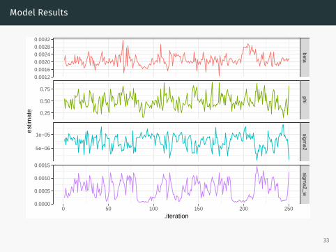
Model Results
betaphi
sigma2
sigma2_w
0 50 100 150 200 250
0.0012
0.0016
0.0020
0.0024
0.0028
0.0032
0.25
0.50
0.75
5e−06
1e−05
0.0000
0.0005
0.0010
0.0015
.iteration
estim
ate
33

Predictions
34°N
34.5°N
35°N
35.5°N
36°N
36.5°N
84°W 82°W 80°W 78°W 76°W
34°N
34.5°N
35°N
35.5°N
36°N
36.5°N
84°W 82°W 80°W 78°W 76°W
0.002
0.004
0.006
0.008bayes_sar_pred
−0.0005
0.0000
0.0005
0.0010
0.0015bayes_sar_resid
34

0.000
0.001
0.002
0.003
0.000 0.001 0.002 0.003
sar_pred
baye
s_sa
r_pr
ed
35
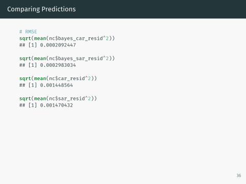
Comparing Predictions
# RMSEsqrt(mean(nc$bayes_car_resid^2))## [1] 0.0002092447
sqrt(mean(nc$bayes_sar_resid^2))## [1] 0.0002983034
sqrt(mean(nc$car_resid^2))## [1] 0.001448564
sqrt(mean(nc$sar_resid^2))## [1] 0.001470432
36

Comparing Parameters
sigma2 sigma2_w
beta phi
2.5e−06 5.0e−06 7.5e−06 1.0e−05 0.00000 0.00025 0.00050 0.00075 0.00100 0.00125
0.0015 0.0020 0.0025 0.2 0.4 0.6 0.8
estimate
model
Stan CAR
Stan SAR
37