LECTURE 17 DIRECT SOLUTIONS TO LINEAR SYSTEMS … · DIRECT SOLUTIONS TO LINEAR SYSTEMS OF...

CE 30125 - Lecture 17

p. 17.1

LECTURE 17

DIRECT SOLUTIONS TO LINEAR SYSTEMS OF ALGEBRAIC EQUATIONS

• Solve the system of equations

• The solution is formally expressed as:

AX B=

a1 1 a1 2 a1 3 a1 4

a2 1 a2 2 a2 3 a2 4

a3 1 a3 2 a3 3 a3 4

a4 1 a4 2 a4 3 a4 4

x1

x2

x3

x4

b1

b2

b3

b4

=

X A 1– B=

CE 30125 - Lecture 2 - Fall 2004

p. 2.2

• Typically it is more efficient to solve for directly without solving for sincefinding the inverse is an expensive (and less accurate) procedure

• Types of solution procedures

• Direct Procedures

• Exact procedures which have infinite precision (excluding roundoff error)

• Suitable when is relatively fully populated/dense or well banded

• A predictable number of operations is required

• Indirect Procedures

• Iterative procedures

• Are appropriate when is

• Large and sparse but not tightly banded

• Very large (since roundoff accumulates more slowly)

• Accuracy of the solution improves as the number of iterations increases

X A 1–

A

A


p. 17.3

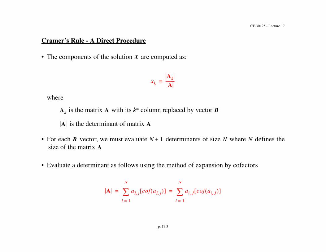
Cramer’s Rule - A Direct Procedure

• The components of the solution are computed as:

where

is the matrix with its kth column replaced by vector

is the determinant of matrix

• For each vector, we must evaluate determinants of size where defines thesize of the matrix

• Evaluate a determinant as follows using the method of expansion by cofactors

X

xk

Ak

A---------=

Ak A B

A A

B N 1+ N NA

A aI j cof aI j j 1=

N

ai J cof ai J i 1=

N

= =


p. 2.4

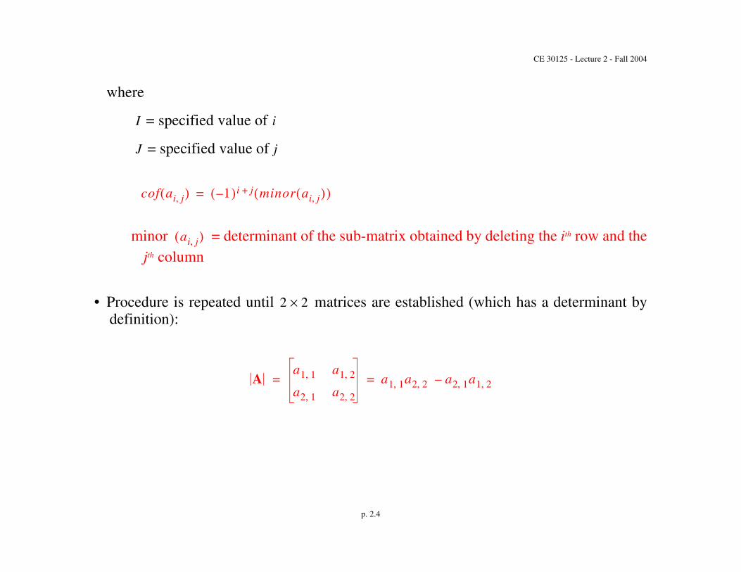
where

= specified value of

= specified value of

minor = determinant of the sub-matrix obtained by deleting the ith row and thejth column

• Procedure is repeated until matrices are established (which has a determinant bydefinition):

I i

J j

cof ai j 1– i j+ minor ai j =

ai j

2 2

Aa1 1 a1 2

a2 1 a2 2

a1 1 a2 2 a2 1 a1 2–= =


p. 17.5

Example

• Evaluate the determinant of

A

det A A

a1 1 a1 2 a1 3

a2 1 a2 2 a2 3

a3 1 a3 2 a3 3

= =

det A a1 1 1– 1 1+ a2 2 a2 3

a3 2 a3 3

a1 2 1– 1 2+ a2 1 a2 3

a3 1 a3 3

+=

a1 3 1– 1 3+ a2 1 a2 2

a3 1 a3 2

+

det A a1 1 +1 a2 2 a3 3 a3 2 a2 3– a1 2 1– a2 1 a3 3 a3 1 a2 3– +=

a1 3 +1 a2 1 a3 2 a3 1 a2 2– +


p. 2.6

• Note that more efficient methods are available to compute the determinant of a matrix.These methods are associated with alternative direct procedures.

• This evaluation of the determinant involves operations

• Number of operations for Cramers’ Rule

system

system

system

• Cramer’s rule is not a good method for very large systems!

• If and no solution! The matrix is singular

• If and infinite number of solutions!

O N 3

O N 4

2 2 O 24 O 16 =

4 4 O 44 O 256 =

8 8 O 84 O 4096 =

A 0= Ak 0 A

A 0= Ak 0=


p. 17.7

Gauss Elimination - A Direct Procedure

• Basic concept is to produce an upper or lower triangular matrix and to then use back-ward or forward substitution to solve for the unknowns.

Example application

• Solve the system of equations

• Divide the first row of and by (pivot element) to get

a1 1 a1 2 a1 3

a2 1 a2 2 a2 3

a3 1 a3 2 a3 3

x1

x2

x3

b1

b2

b3

=

A B a1 1

1 a'1 2 a'1 3

a2 1 a2 2 a2 3

a3 1 a3 2 a3 3

x1

x2

x3

b'1b2

b3

=


p. 2.8

• Now multiply row 1 by and subtract from row 2

and then multiply row 1 by and subtract from row 3

• Now divide row 2 by (pivot element)

a2 1

a3 1

1 a'1 2 a'1 3

0 a'2 2 a'2 3

0 a'3 2 a'3 3

x1

x2

x3

b'1b'2b'3

=

a'2 2

1 a'1 2 a'1 3

0 1 a''2 3

0 a'3 2 a'3 3

x1

x2

x3

b'1b''2b'3

=


p. 17.9

• Now multiply row 2 by and subtract from row 3 to get

• Finally divide row 3 by (pivot element) to complete the triangulation procedureand results in the upper triangular matrix

• We have triangularized the coefficient matrix simply by taking linear combinations ofthe equations

a'3 2

1 a'1 2 a'1 3

0 1 a''2 3

0 0 a''3 3

x1

x2

x3

b'1b''2b''3

=

a''3 3

1 a'1 2 a'1 3

0 1 a''2 3

0 0 1

x1

x2

x3

b'1b''2b'''3

=


p. 2.10

• We can very conveniently solve the upper triangularized system of equations

• We apply a backward substitution procedure to solve for the components of

• We can also produce a lower triangular matrix and use a forward substitution procedure

1 a'1 2 a'1 3

0 1 a''2 3

0 0 1

x1

x2

x3

b'1b''2b'''3

=

X

x3 b'''3=

x2 a''2 3 x3+ b''2= x2 b''2 a''2 3 x3–=

x1 a'1 2 x2 a'1 3 x3+ + b'1= x1 b'1 a'1 2 x2 a'1 3 x3––=


p. 17.11

• Number of operations required for Gauss elimination

• Triangularization

• Backward substitution

• Total number of operations for Gauss elimination equals versus forCramer’s rule

• Therefore we save operations as compared to Cramer’s rule

Gauss-Jordan Elimination - A Direct Procedure

• Gauss Jordan elimination is an adaptation of Gauss elimination in which both elementsabove and below the pivot element are cleared to zero the entire column except thepivot element become zeroes

• No backward/forward substitution is necessary

13---N3

12---N2

O N 3 O N 4

O N

1 0 0 0

0 1 0 0

0 0 1 0

0 0 0 1

x1

x2

x3

x4

b1

b2

b3

b4

=


p. 2.12

Matrix Inversion by Gauss-Jordan Elimination

• Given , find such that

where = identity matrix =

• Procedure is similar to finding the solution of except that the matrix

assumes the role of vector and matrix serves as vector

• Therefore we perform the same operations on and

A A 1–

AA 1– I

I

1 0 0 0 0 0

0 1 0 0 0 0

0 0 1 0 0 0

0 0 0 1 0 0

0 0 0 0 1 0

0 0 0 0 0 1

AX B= A 1–

X I B

A I


p. 17.13

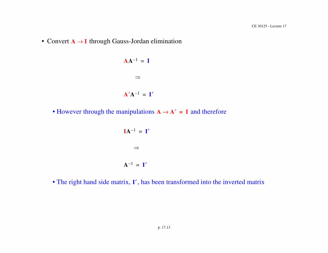
• Convert through Gauss-Jordan elimination

• However through the manipulations and therefore

• The right hand side matrix, , has been transformed into the inverted matrix

A I

AA 1– I=

AA 1– I=

A A I=

IA 1– I=

A 1– I=

I


p. 2.14

• Notes:

• Inverting a diagonal matrix simply involves computing reciprocals

• Inverse of the product relationship

A

a11 0 0

0 a22 0

0 0 a33

=

A 1–

1/a11 0 0

0 1/a22 0

0 0 1/a33

=

AA 1– I=

A1A2A3 1– A31– A2

1– A11–=


p. 17.15

Gauss Elimination Type Solutions to Banded Matrices

Banded matrices

• Have non-zero entries contained within a defined number of positions to the left andright of the diagonal (bandwidth)

INSERT FIGURE NO. 122

x x xo o o o o o o o o

x x x o o o o o o o ox

x o o o o o oxo o x x

x o o o o ox x xooo

o x x o x o x o o o o o

o o o xx x x o x o o o

o o o x o x x x o x o o

o o o o o o x x x xo

o

o o o o o x o x x x x

o o o o o o x o x x

o

x o

o o o o o o o o x x x x

o o o o o o o o x x xo

o o o x x o x

o o x x x x o

o x x o x xo

x x o xox

x x o x o x o

o x x o

x x x o

o x x xo

o

x o x x x x

x x o

o x xo x o

x x x

o

o x x

o x

x o x o

x x o o

x x o o

NxN System Compact Diagonal

halfbandwidth bandwidthM

stored as

M + 12

bandwidth M = 7

= 4

storage required = N2 storage required = NM


p. 2.16

• Notes on banded matrices

• The advantage of banded storage mode is that we avoid storing and manipulatingzero entries outside of the defined bandwidth

• Banded matrices typically result from finite difference and finite element methods(conversion from p.d.e. algebraic equations)

• Compact banded storage mode can still be sparse (this is particularly true for largefinite difference and finite element problems)

Savings on storage for banded matrices

• for full storage versus for banded storage

where = the size of the matrix and = the bandwidth

• Examples:

N M full banded ratio

400 20 160,000 8,000 20

106 103 1012 109 1000

N2 NM

N M


p. 17.17

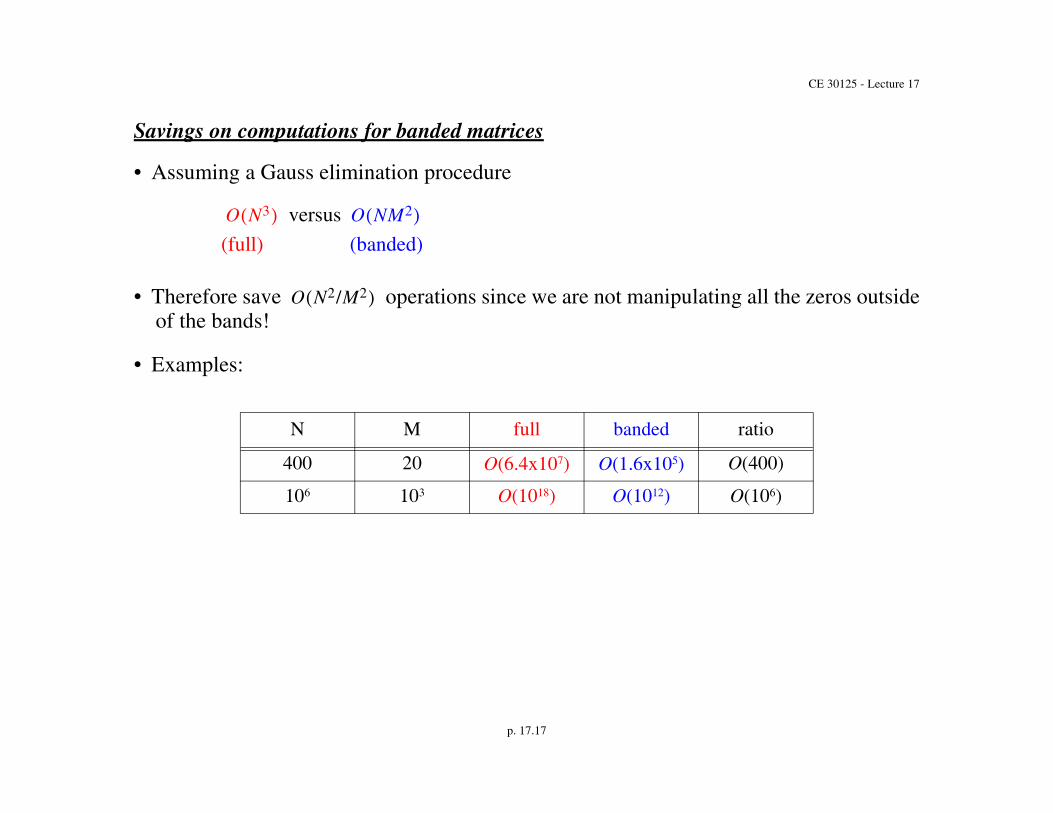
Savings on computations for banded matrices

• Assuming a Gauss elimination procedure

versus

(full) (banded)

• Therefore save operations since we are not manipulating all the zeros outsideof the bands!

• Examples:

N M full banded ratio

400 20 O(6.4x107) O(1.6x105) O(400)

106 103 O(1018) O(1012) O(106)

O N3 O NM2

O N2/M2


p. 2.18

Symmetrical banded matrices

• Substantial savings on both storage and computations if we use a banded storage mode

• Even greater savings (both storage and computations) are possible if the matrix issymmetrical

• Therefore if we need only store and operate on half the bandwidth in abanded matrix (half the matrix in a full storage mode matrix)

INSERT FIGURE NO. 123a

A

aij aji=

(M + 1)/2

store only half

(M + 1)/2


p. 17.19

Alternative Compact Storage Modes for Direct Methods

• Skyline method defines an alternative compact storage procedure for symmetricalmatrices

• The skyline goes below the last non-zero element in a column

INSERT FIGURE NO. 123b

a11 a12

a22 a23

a33 a34

a44

o

a14

a45

o

o

o

a55

o

o

a36

a46

a56

a66

symmetrical

oSkyline goes above the lastnon-zero element in a column


p. 2.20

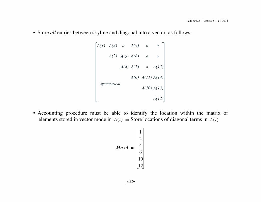
• Store all entries between skyline and diagonal into a vector as follows: INSERT FIGURE NO. 124

• Accounting procedure must be able to identify the location within the matrix ofelements stored in vector mode in Store locations of diagonal terms in

o o

symmetrical

A(1) oA(3) A(9)

A(2) A(5) A(8) o o

A(4) A(7) o A(15)

A(6) A(14)A(11)

A(13)A(10)

A(12)

A i A i

MaxA

1

2

4

6

10

12

=


p. 17.21

• Savings in storage and computation time due to the elimination of the additional zeroes

e.g. storage savings:

• Program COLSOL (Bathe and Wilson) available for skyline storage solution

full symmetrical banded skyline

N2 36= M 1+2

-------------- N

7 1+2

------------ 6 24= = 15


p. 2.22

Problems with Gauss Elimination Procedures

Inaccuracies originating from the pivot elements

• The pivot element is the diagonal element which divides the associated row

• As more pivot rows are processed, the number of times a pivot element has been modi-fied increases.

• Sometimes a pivot element can become very small compared to the rest of the elementsin the pivot row

• Pivot element will be inaccurate due to roundoff

• When the pivot element divides the rest of the pivot row, large inaccurate numbersresult across the pivot row

• Pivot row now subtracts (after being multiplied) from all rows below the pivot row,resulting in propagation of large errors throughout the matrix!

Partial pivoting

• Always look below the pivot element and pick the row with the largest value and switchrows


p. 17.23

Complete pivoting

• Look at all columns and all rows to the right/below the pivot element and switch so thatthe largest element possible is in the pivot position.

• For complete pivoting, you must change the order of the variable array

• Pivoting procedures give large diagonal elements

• minimize roundoff error

• increase accuracy

• Pivoting is not required when the matrix is diagonally dominant

• A matrix is diagonally dominant when the absolute values of the diagonal terms isgreater than the sum of the absolute values of the off diagonal terms for each row

LECTURE 17 DIRECT SOLUTIONS TO LINEAR SYSTEMS … · DIRECT SOLUTIONS TO LINEAR SYSTEMS OF...

Documents

Transcript of LECTURE 17 DIRECT SOLUTIONS TO LINEAR SYSTEMS … · DIRECT SOLUTIONS TO LINEAR SYSTEMS OF...