Lecture 15 Perron-Frobenius Theoryyaroslavvb.com/papers/notes/perron-frobenius-theory.pdf · ·...

EE363 Winter 2005-06

Lecture 15Perron-Frobenius Theory

• Positive and nonnegative matrices and vectors

• Perron-Frobenius theorems

• Markov chains

• Economic growth

• Population dynamics

• Max-min and min-max characterization

• Power control

• Linear Lyapunov functions

• Metzler matrices

15–1

Positive and nonnegative vectors and matrices

we say a matrix or vector is

• positive (or elementwise positive) if all its entries are positive

• nonnegative (or elementwise nonnegative) if all its entries arenonnegative

we use the notation x > y (x ≥ y) to mean x − y is elementwise positive(nonnegative)

warning: if A and B are square and symmetric, A ≥ B can mean:

• A − B is PSD (i.e., zTAz ≥ zTBz for all z), or

• A − B elementwise positive (i.e., Aij ≥ Bij for all i, j)

in this lecture, > and ≥ mean elementwise

Perron-Frobenius Theory 15–2

Application areas

nonnegative matrices arise in many fields, e.g.,

• economics

• population models

• graph theory

• Markov chains

• power control in communications

• Lyapunov analysis of large scale systems


Basic facts

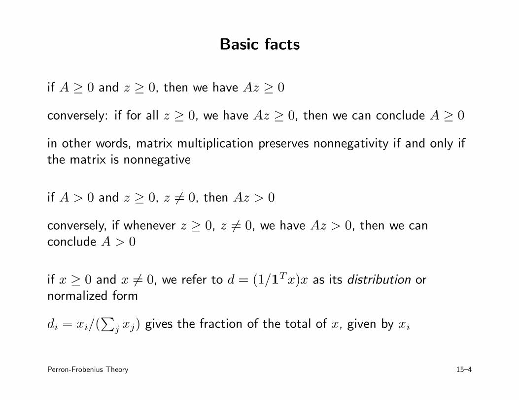
if A ≥ 0 and z ≥ 0, then we have Az ≥ 0

conversely: if for all z ≥ 0, we have Az ≥ 0, then we can conclude A ≥ 0

in other words, matrix multiplication preserves nonnegativity if and only ifthe matrix is nonnegative

if A > 0 and z ≥ 0, z 6= 0, then Az > 0

conversely, if whenever z ≥ 0, z 6= 0, we have Az > 0, then we canconclude A > 0

if x ≥ 0 and x 6= 0, we refer to d = (1/1Tx)x as its distribution ornormalized form

di = xi/(∑

j xj) gives the fraction of the total of x, given by xi


Regular nonnegative matrices

suppose A ∈ Rn×n, with A ≥ 0

A is called regular if for some k ≥ 1, Ak > 0

meaning: form directed graph on nodes 1, . . . , n, with an arc from j to iwhenever Aij > 0

then (Ak)ij > 0 if and only if there is a path of length k from j to i

A is regular if for some k there is a path of length k from every node toevery other node


examples:

• any positive matrix is regular

•

[

1 10 1

]

and

[

0 11 0

]

are not regular

•

1 1 00 0 11 0 0

is regular


Perron-Frobenius theorem for regular matrices

suppose A ∈ Rn×n is nonnegative and regular, i.e., Ak > 0 for some k

then

• there is an eigenvalue λpf of A that is real and positive, with positiveleft and right eigenvectors

• for any other eigenvalue λ, we have |λ| < λpf

• the eigenvalue λpf is simple, i.e., has multiplicity one, and correspondsto a 1 × 1 Jordan block

the eigenvalue λpf is called the Perron-Frobenius (PF) eigenvalue of A

the associated positive (left and right) eigenvectors are called the (left andright) PF eigenvectors (and are unique, up to positive scaling)


Perron-Frobenius theorem for nonnegative matrices

suppose A ∈ Rn×n and A ≥ 0

then

• there is an eigenvalue λpf of A that is real and nonnegative, withassociated nonnegative left and right eigenvectors

• for any other eigenvalue λ of A, we have |λ| ≤ λpf

λpf is called the Perron-Frobenius (PF) eigenvalue of A

the associated nonnegative (left and right) eigenvectors are called (left andright) PF eigenvectors

in this case, they need not be unique, or positive


Markov chains

we consider stochastic process X(0), X(1), . . . with values in {1, . . . , n}

Prob(X(t + 1) = i|X(t) = j) = Pij

P is called the transition matrix ; clearly Pij ≥ 0

let p(t) ∈ Rn be the distribution of X(t), i.e., pi(t) = Prob(X(t) = i)

then we have p(t + 1) = Pp(t)

note: standard notation uses transpose of P , and row vectors forprobability distributions

P is a stochastic matrix, i.e., P ≥ 0 and 1TP = 1

T

so 1 is a left eigenvector with eigenvalue 1, which is in fact the PFeigenvalue of P


Equilibrium distribution

let π denote a PF (right) eigenvector of P , with π ≥ 0 and 1Tπ = 1

since Pπ = π, π corresponds to an invariant distribution or equilibrium

distribution of the Markov chain

now suppose P is regular, which means for some k, P k > 0

since (P k)ij is Prob(X(t + k) = i|X(t) = j), this means there is positiveprobability of transitioning from any state to any other in k steps

since P is regular, there is a unique invariant distribution π, which satisfiesπ > 0

the eigenvalue 1 is simple and dominant, so we have p(t) → π, no matterwhat the initial distribution p(0)

in other words: the distribution of a regular Markov chain always convergesto the unique invariant distribution


Rate of convergence to equilibrium distribution

rate of convergence to equilibrium distribution depends on second largesteigenvalue magnitude, i.e.,

µ = max{|λ2|, . . . , |λn|}

where λi are the eigenvalues of P , and λ1 = λpf = 1

(µ is sometimes called the SLEM of the Markov chain)

the mixing time of the Markov chain is given by

T =1

log(1/µ)

(roughly, number of steps over which deviation from equilibriumdistribution decreases by factor e)


Dynamic interpretation

consider x(t + 1) = Ax(t), with A ≥ 0 and regular

then by PF theorem, λpf is the unique dominant eigenvalue

let v, w > 0 be the right and left PF eigenvectors of A, with 1Tv = 1,

wTv = 1

then as t → ∞, (λ−1pf A)t → vwT

for any x(0) ≥ 0, x(0) 6= 0, we have

1

1Tx(t)x(t) → v

as t → ∞, i.e., the distribution of x(t) converges to v

we also have xi(t + 1)/xi(t) → λpf, i.e., the one-period growth factor ineach component always converges to λpf


Economic growth

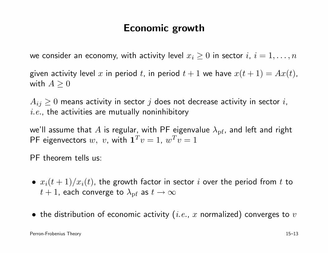
we consider an economy, with activity level xi ≥ 0 in sector i, i = 1, . . . , n

given activity level x in period t, in period t + 1 we have x(t + 1) = Ax(t),with A ≥ 0

Aij ≥ 0 means activity in sector j does not decrease activity in sector i,i.e., the activities are mutually noninhibitory

we’ll assume that A is regular, with PF eigenvalue λpf, and left and rightPF eigenvectors w, v, with 1

Tv = 1, wTv = 1

PF theorem tells us:

• xi(t + 1)/xi(t), the growth factor in sector i over the period from t tot + 1, each converge to λpf as t → ∞

• the distribution of economic activity (i.e., x normalized) converges to v


• asymptotically the economy exhibits (almost) balanced growth, by thefactor λpf, in each sector

these hold independent of the original economic activity, provided it isnonnegative and nonzero

what does left PF eigenvector w mean?

for large t we havex(t) ∼ λt

pfwTx(0)v

where ∼ means we have dropped terms small compared to dominant term

so asymptotic economic activity is scaled by wTx(0)

in particular, wi gives the relative value of activity i in terms of long termeconomic activity


Population model

xi(t) denotes number of individuals in group i at period t

groups could be by age, location, health, marital status, etc.

population dynamics is given by x(t + 1) = Ax(t), with A ≥ 0

Aij gives the fraction of members of group j that move to group i, or thenumber of members in group i created by members of group j (e.g., inbirths)

Aij ≥ 0 means the more we have in group j in a period, the more we havein group i in the next period

• if∑

i Aij = 1, population is preserved in transitions out of group j

• we can have∑

i Aij > 1, if there are births (say) from members ofgroup j

• we can have∑

i Aij < 1, if there are deaths or attrition in group j


now suppose A is regular

• PF eigenvector v gives asymptotic population distribution

• PF eigenvalue λpf gives asymptotic growth rate (if > 1) or decay rate(if < 1)

• wTx(0) scales asymptotic population, so wi gives relative value ofinitial group i to long term population


Path count in directed graph

we have directed graph on n nodes, with adjacency matrix A ∈ Rn×n

Aij =

{

1 there is an edge from node j to node i0 otherwise

(

Ak)

ijis number of paths from j to i of length k

now suppose A is regular

then for large k,

Ak ∼ λkpfvwT = λk

pf(1Tw)v(w/1Tw)T

(∼ means: keep only dominant term)

v, w are right, left PF eigenvectors, normalized as 1Tv = 1, wTv = 1


total number of paths of length k: 1TAk

1 ≈ λkpf(1

Tw)

for k large, we have (approximately)

• λpf is factor of increase in number of paths when length increases by one

• vi: fraction of length k paths that end at i

• wj/1Tw: fraction of length k paths that start at j

• viwj/1Tw: fraction of length k paths that start at j, end at i

• vi measures importance/connectedness of node i as a sink

• wj/1Tw measures importance/connectedness of node j as a source


(Part of) proof of PF theorem for positive matrices

suppose A > 0, and consider the optimization problem

maximize δsubject to Ax ≥ δx for some x ≥ 0, x 6= 0

note that we can assume 1Tx = 1

interpretation: with yi = (Ax)i, we can interpret yi/xi as the ‘growthfactor’ for component i

problem above is to find the input distribution that maximizes theminimum growth factor

let λ0 be the optimal value of this problem, and let v be an optimal point,i.e., v ≥ 0, v 6= 0, and Av ≥ λ0v


we will show that λ0 is the PF eigenvalue of A, and v is a PF eigenvector

first let’s show Av = λ0v, i.e., v is an eigenvector associated with λ0

if not, suppose that (Av)k > λ0vk

now let’s look at v = v + εek

we’ll show that for small ε > 0, we have Av > λ0v, which means thatAv ≥ δv for some δ > λ0, a contradiction

for i 6= k we have

(Av)i = (Av)i + Aikε > (Av)i ≥ λ0vi = λ0vi

so for any ε > 0 we have (Av)i > λ0vi

(Av)k − λ0vk = (Av)k + Akkε − λ0vk − λ0ε

= (Av)k − λ0vk − ε(λ0 − Akk)


since (Av)k − λ0vk > 0, we conclude that for small ε > 0,(Av)k − λ0vk > 0

to show that v > 0, suppose that vk = 0

from Av = λ0v, we conclude (Av)k = 0, which contradicts Av > 0(which follows from A > 0, v ≥ 0, v 6= 0)

now suppose λ 6= λ0 is another eigenvalue of A, i.e., Az = λz, wherez 6= 0

let |z| denote the vector with |z|i = |zi|

since A ≥ 0 we have A|z| ≥ |Az| = |λ||z|

from the definition of λ0 we conclude |λ| ≤ λ0

(to show strict inequality is harder)


Max-min ratio characterization

proof shows that PF eigenvalue is optimal value of optimization problem

maximize mini(Ax)i

xi

subject to x > 0

and that PF eigenvector v is optimal point:

• PF eigenvector v maximizes the minimum growth factor overcomponents

• with optimal v, growth factors in all components are equal (to λpf)

in other words: by maximizing minimum growth factor, we actually achievebalanced growth


Min-max ratio characterization

a related problem is

minimize maxi(Ax)i

xi

subject to x > 0

here we seek to minimize the maximum growth factor in the coordinates

the solution is surprising: the optimal value is λpf and the optimal x is thePF eigenvector v

• if A is nonnegative and regular, and x > 0, the n growth factors(Ax)i/xi ‘straddle’ λpf: at least one is ≥ λpf, and at least one is ≤ λpf

• when we take x to be the PF eigenvector v, all the growth factors areequal, and solve both max-min and min-max problems


Power control

we consider n transmitters with powers P1, . . . , Pn > 0, transmitting to nreceivers

path gain from transmitter j to receiver i is Gij > 0

signal power at receiver i is Si = GiiPi

interference power at receiver i is Ii =∑

k 6=i GikPk

signal to interference ratio (SIR) is

Si/Ii =GiiPi

∑

k 6=i GikPk

how do we set transmitter powers to maximize the minimum SIR?


we can just as well minimize the maximum interference to signal ratio, i.e.,solve the problem

minimize maxi(GP )i

Pi

subject to P > 0

where

Gij =

{

Gij/Gii i 6= j0 i = j

since G2 > 0, G is regular, so solution is given by PF eigenvector of G

PF eigenvalue λpf of G is the optimal interference to signal ratio, i.e.,maximum possible minimum SIR is 1/λpf

with optimal power allocation, all SIRs are equal

note: G is the matrix of ratios of interference to signal path gains


Nonnegativity of resolvent

suppose A is nonnegative, with PF eigenvalue λpf, and λ ∈ R

then (λI − A)−1 exists and is nonnegative, if and only if λ > λpf

for any square matrix A the power series expansion

(λI − A)−1 =1

λI +

1

λ2A +

1

λ3A2 + · · ·

converges provided |λ| is larger than all eigenvalues of A

if λ > λpf, this shows that (λI − A)−1 is nonnegative

to show converse, suppose (λI − A)−1 exists and is nonnegative, and letv 6= 0, v ≥ 0 be a PF eigenvector of A

then we have

(λI − A)−1v =1

λ − λpfv ≥ 0

and it follows that λ > λpf


Equilibrium points

consider x(t + 1) = Ax(t) + b, where A and b are nonnegative

equilibrium point is given by xeq = (I − A)−1b

by resolvent result, if A is stable, then (I − A)−1 is nonnegative, soequilibrium point xeq is nonnegative for any nonnegative b

moreover, equilibrium point is monotonic function of b: for b ≥ b, we havexeq ≥ xeq

conversely, if system has a nonnegative equilibrium point, for everynonnegative choice of b, then we can conclude A is stable


Iterative power allocation algorithm

we consider again the power control problem

suppose γ is the desired or target SIR

simple iterative algorithm: at each step t,

1. first choose Pi so that

GiiPi∑

k 6=i GikPk(t)= γ

Pi is the transmit power that would make the SIR of receiver i equal toγ, assuming none of the other powers change

2. set Pi(t + 1) = Pi + σi, where σi > 0 is a parameteri.e., add a little extra power to each transmitter)


each receiver only needs to know its current SIR to adjust its power: ifcurrent SIR is α dB below (above) γ, then increase (decrease) transmitterpower by α dB, then add the extra power σ

i.e., this is a distributed algorithm

question: does it work? (we assume that P (0) > 0)

answer: yes, if and only if γ is less than the maximum achievable SIR, i.e.,γ < 1/λpf(G)

to see this, algorithm can be expressed as follows:

• in the first step, we have P = γGP (t)

• in the second step we have P (t + 1) = P + σ

and so we haveP (t + 1) = γGP (t) + σ

a linear system with constant input


PF eigenvalue of γG is γλpf, so linear system is stable if and only ifγλpf < 1

power converges to equilibrium value

Peq = (I − γG)−1σ

(which is positive, by resolvent result)

now let’s show this equilibrium power allocation achieves SIR at least γ foreach receiver

we need to verify γGPeq ≤ Peq, i.e.,

γG(I − γG)−1σ ≤ (I − γG)−1σ

or, equivalently,

(I − γG)−1σ − γG(I − γG)−1σ ≥ 0

which holds, since the lefthand side is just σ


Linear Lyapunov functions

suppose A ≥ 0

then Rn+ is invariant under system x(t + 1) = Ax(t)

suppose c > 0, and consider the linear Lyapunov function V (z) = cTz

if V (Az) ≤ δV (z) for some δ < 1 and all z ≥ 0, then V proves(nonnegative) trajectories converge to zero

fact: a nonnegative regular system is stable if and only if there is a linearLyapunov function that proves it

to show the ‘only if’ part, suppose A is stable, i.e., λpf < 1

take c = w, the (positive) left PF eigenvector of A

then we have V (Az) = wTAz = λpfwTz, i.e., V proves all nonnegative

trajectories converge to zero


Weighted `1-norm Lyapunov function

to make the analysis apply to all trajectories, we can consider the weightedsum absolute value (or weighted `1-norm) Lyapunov function

V (z) =

n∑

i=1

wi|zi| = wT |z|

then we have

V (Az) =

n∑

i=1

wi|(Az)i| ≤

n∑

i=1

wi(A|z|)i = wTA|z| = λpfwT |z|

which shows that V decreases at least by the factor λpf

conclusion: a nonnegative regular system is stable if and only if there is aweighted sum absolute value Lyapunov function that proves it


SVD analysis

suppose A ∈ Rm×n, A ≥ 0

then ATA ≥ 0 and AAT ≥ 0 are nonnegative

hence, there are nonnegative left & right singular vectors v1, w1 associatedwith σ1

in particular, there is an optimal rank-1 approximation of A that isnonnegative

if ATA, AAT are regular, then we conclude

• σ1 > σ2, i.e., maximum singular value is isolated

• associated singular vectors are positive: v1 > 0, w1 > 0


Continuous time results

we have already seen that Rn+ is invariant under x = Ax if and only if

Aij ≥ 0 for i 6= j

such matrices are called Metzler matrices

for a Metzler matrix, we have

• there is an eigenvalue λmetzler of A that is real, with associatednonnegative left and right eigenvectors

• for any other eigenvalue λ of A, we have <λ ≤ λmetzler

i.e., the eigenvalue λmetzler is dominant for system x = Ax

• if λ > λmetzler, then (λI − A)−1 ≥ 0


the analog of the stronger Perron-Frobenius results:

if (τI + A)k > 0, for some τ and some k, then

• the left and right eigenvectors associated with eigenvalue λmetzler of Aare positive

• for any other eigenvalue λ of A, we have <λ < λmetzler

i.e., the eigenvalue λmetzler is strictly dominant for system x = Ax


Derivation from Perron-Frobenius Theory

suppose A is Metzler, and choose τ s.t. τI + A ≥ 0(e.g., τ = 1 − mini Aii)

by PF theory, τI + A has PF eigenvalue λpf, with associated right and lefteigenvectors v ≥ 0, w ≥ 0

from (τI + A)v = λpfv we get Av = (λpf − τ)v = λ0v, and similarly for w

we’ll show that <λ ≤ λ0 for any eigenvalue λ of A

suppose λ is an eigenvalue of A

suppose τ + λ is an eigenvalue of τI + A

by PF theory, we have |τ + λ| ≤ λpf = τ + λ0

this means λ lies inside a circle, centered at −τ , that passes through λ0

which implies <λ ≤ λ0


Linear Lyapunov function

suppose x = Ax is stable, and A is Metzler, with (τI + A)k > 0 for someτ and some k

we can show that all nonnegative trajectories converge to zero using alinear Lyapunov function

let w > 0 be left eigenvector associated with dominant eigenvalue λmetzler

then with V (z) = wTz we have

V (z) = wTAz = λmetzlerwTz = λmetzlerV (z)

since λmetzler < 0, this proves wTz → 0


Lecture 15 Perron-Frobenius Theoryyaroslavvb.com/papers/notes/perron-frobenius-theory.pdf · ·...

Documents

Transcript of Lecture 15 Perron-Frobenius Theoryyaroslavvb.com/papers/notes/perron-frobenius-theory.pdf · ·...