Lecture 14

Nonpremixed Turbulent Combustion:

The Flamelet Concept

14.-1

Models in nonpremixed turbulent combustion are often based on the presumedshape pdf approach.

This requires the knowledge of the Favre mean mixture fraction and its variance at position x and time t.

A of the mixture fraction equation and using the gradient transport assumption led to the equation for the Favre mean mixture fraction

Molecular diffusion is much smaller than the turbulent diffusion, and has therefore been neglected.

14.-2

In addition to the mean mixture fraction we have derived an equation for the Favre variance of the mixture fraction

where the gradient transport assumption

has again been used in the production term, second term of the r.h.s.

For the turbulent flux of the mixture fraction variance the gradient transport assumption

can also be used.

14.-3

In

the mean scalar dissipation rate appears, which as introduced in Lecture 10 will be modeled as

where the time scale ratio cχ is assumed to be a constant.

14.-4

In the model

Janicka and Peters (1982) found that a value of cχ=2.0 would predict the decay of scalar variance in an inert jet of methane very well.

Overholt and Pope (1996) and Juneja and Pope (1996) performing DNS studiesof one and two passive scalar mixing find an increase of cχ with Reynolds number and steady state values around 2.0 and 3.0, respectively.

In the numerical simulations of Diesel engine combustion, to be presented in Lecture 15, a value of cχ=2.0 has been used.

14.-5

In many cases, as in turbulent jet diffusion flames in air, zero gradientboundary conditions, except at the inlet, can be imposed.

If the simplifying assumptions mentioned in Section 3.9 of Lecture 3 can be introduced the enthalpy h can be related to the mixture fraction by the linear coupling relation

which also holds for the mean values

and no additional equation for the enthalpy is required.

14.-6

In and

h2 is the enthalpy of the air and h1 that of the fuel.

A more general formulation is needed, if different boundary conditions have to be applied for the Favre mean mixture fraction and enthalpy or if heat loss due to radiation or unsteady pressure changes must be accounted for.

Then an equation for the Favre mean enthalpy as an additional variable must be solved.

14.-7

This equation can be obtained from the enthalpy equation

by averaging

again a gradient transport equation for the correlation has been introduced.

14.-8

The term describing temporal mean pressure changes has been retained, because it is important for the modeling of combustion in internal combustion engines operating under nonpremixed conditions, such as the Diesel engine.

The mean volumetric heat exchange term must also be retained in many applications where radiative heat exchange has an influence on the local enthalpybalance.

Changes of the mean enthalpy also occur due to convective heat transfer at the boundaries or due to the evaporation of a liquid fuel.

Temperature changes due to radiation within the flamelet structure also have a strong influence on the prediction of NOx formation (cf. Pitsch et al. ,1998).

14.-9

Presumed Shape Pdf Approach

The modelling eqations can be used to calculate the mean mixture fraction and the mixture fraction variance at each point of the turbulent flow field, provided that the density field is known.

In addition, of course, equations for the turbulent flow field, the Reynolds stress equations (or the equation for the turbulent kinetic energy) and the equation for the dissipation must be solved.

14.-10

In this approach a suitable two-parameter probability density function is "presumed" in advance, thereby fixing the functional form of the pdf by relating the two parameters in terms of the known values of the mean mixture fraction and its variance at each point of the flow field.

Since in a two-feed system the mixture fraction Z varies between Z = 0 andZ = 1, the beta function pdf is widely used for the Favre pdf in nonpremixedturbulent combustion.

14.-11

The beta-function pdf has the form

Here Γ is the gamma function.

The two parameters α and β are related to the Favre mean mixture fraction and its variance by

where

14.-12

The beta-function plotted for different combinations of its parameters

It can be shown that in the limit of very small (large γ) it approaches a Gaussian distribution.

14.-13

For α <1 it develops a singularity at Z = 0 and for β < 1 a singularity at Z = 1.

Despite of its surprising flexibility, it is unable to describe distributions witha singularity at Z = 0 or Z = 1 and an additional intermediate maximum in the range 0 < Z < 1.

14.-14

By the presumed shape pdf approach means of any quantity that depends only on the mixture fraction can be calculated.

For instance, the mean value of ψi can be obtained from

A further quantity of interest is the mean density.

Since Favre averages are considered, one must take the Favre average of ρ-1, which leads to

14.-15

With

and the Burke-Schumann solution the Conserved´Scalar Equilibrium Model for nonpremixed combustion is formulated.

It is based on a closed set of equations which do not require any further chemical input other than the assumption of infinitely fast chemistry.

It may therefore be used as an initial guess in a calculation where the Burke-Schumann solution or the equilibrium solution later on is replaced by the solution of the flamelet equations to account for non-equilibrium effects.

14.-16

The Round Turbulent Jet Diffusion Flame

In many applications fuel enters into the combustion chamber as a turbulent jet,with or without swirl.

To provide an understanding of the basic properties of jet diffusion flames, we will consider here the easiest case, the axisymmetric jet flame without buoyancy, for which we can obtain approximate analytical solutions.

This will enable us to determine, for instance, the flame length.

The flame length is defined as the distance from the nozzle to the point on the centerline of the flame where the mean mixture fraction is equal to Zst.

14.-17

The flow configuration for the round turbulent jet flame

14.-18

Using Favre averaging and the the boundary layer assumption we obtain a system of two-dimensional axisymmetric equations

continuity

momentum in x-direction

mean mixture fraction

14.-19

We have neglected molecular as compared to turbulent transport terms.

Turbulent transport was modeled by the gradient flux approximation.

For the scalar flux we have replaced Dt by introducing the turbulent Schmidt number Sct=νt/Dt.

For simplicity, we will not consider equations for the turbulent kinetic energy and its dissipation or the mixture fraction variance but seek an approximate solution byintroducing a model for the turbulent viscosity νt.

Details may be found in Peters and Donnerhack (1981).

14.-20

As for the laminar solution of Lecture 9 for the round diffusion flame the dimensionality of the problem will again be reduced by introducing the similarity transformation

which contains a density transformation defining the density weighted radialco-ordinate.

The new axial co-ordinate ξ starts from the virtual origin of the jet located at x = - x0.

14.-21

Introducing a stream function ψ by

the continuity equation

is satisfied.

In terms of the non-dimensional stream function F(η) defined by

the axial and radial velocity components may now be expressed as

14.-22

Here νtr is the eddy viscosity of a constant density jet, used as a reference value.

Differently from the laminar flame, where ν is a molecular property,νtr has been fitted (cf. Peters and Donnerhack (1981) to experimental data as

For the mixture fraction the ansatz

is introduced, where stands for the Favre mean mixture fraction on the centerline.

14.-23

The system of equation for the turbulent round jet has the same similarity solution as the one derived in Section 9.2 of Lecture 9.

Here we approximate the Chapman-Rubesin parameter, however, as:

In order to derive an analytical solution it must be assumed that C is a constant in the entire jet.

14.-24

With a constant value of C and if the Schmidt number is replaced by a turbulent Schmidt number Sct one obtains the system of differential equations

and its solution

14.-255

The solution reads

where the jet spreading parameter is now

obtained from the requirement of integral momentum conservation along the axialdirection.

14.-26

Similarly, conservation of the mixture fraction integral across the jet yields the mixture fraction on the centerline

such that the mixture fraction profile is given by

From this equation the flame length L can be calculated by setting

We get

14.-27

Experimental data by Hawthorne et al. (1949) suggest that the flame length Lshould scale as

This fixes the turbulent Schmidt number as Sct=0.71 and the Chapman-Rubesinparameter as

When this is introduced into the solution, one obtains the centerline velocity as

14.-28

The distance of the virtual origin from x = 0 may be estimatedby setting

in

so that

As an example for the flame length, we set the molecular weight at stoichiometricmixture equal to that of nitrogen, thereby estimating the density ratio ρ0 / ρst from

14.-29

The flame length may then be calculated from

with Zst = 0.055 as L ~ 200 d

In large turbulent diffusion flames buoyancy influences the turbulentflow field and thereby the flame length.

In order to derive a scaling law for that case, Peters and Göttgens (1991) have integrated the boundary layer equations for momentum and mixture fraction fora vertical jet flame over the radial direction in order to obtain first orderdifferential equations in terms of the axial co-ordinate for cross-sectional averages of the axial velocity and the mixture fraction.

14.-30

Since turbulent transport disappears entirely due to averaging, an empirical model for the entrainment coefficient β is needed, which relates the half-width b of the jet to the axial co-ordinate as

By comparison with the similarity solution for a non-buoyant jet β was determined as

Details of the derivation may be found in Peters and Göttgens (1991).

14.-31

The predicted flame length of propane flames is compared with measurementsfrom Sønju and Hustad (1984).

For Froude numbers smaller than 105 the data show a Froude number scaling asFr1/5, which corresponds to a balance of the second term on thel.h.s. with the term on the r.h.s.

14.-32

For Froude numbers larger than 106 the flame length becomes Froude number independent equal to the value calculated from

14.-33

Experimental Data from Turbulent Jet Diffusion Flames

There is a large body of experimental data on single point measurements using Laser Rayleigh and Raman scattering techniques combined with Laser-Induced Fluorescence (LIF).

Since a comprehensive review on the subject by Masri et al. (1996) isavailable, it suffices to present as an example the results by Barlow et al. (1990) obtained by the combined Raman-Rayleigh-LIF technique.

The fuel stream of the two flames that were investigated consisted of a mixture of 78 mole % H2 and 22 mole % argon, the nozzle inner diameter d was 5.2 mm and the co-flow air velocity was 9.2 m/s.

The resulting flame length was approximately L = 60 d.

14.-34

Two cases of exit velocities were analyzed, but only the case B with u0 = 150 m/swill be considered here.

The stable species H2, O2, N2, and H2O were measured using Raman-scattering at a single point with light from a flash-lamp pumped dye laser.

In addition, quantitative OH radical concentrations from LIF measurementswere obtained by using the instantaneous one-point Raman data to calculatequenching corrections for each laser shot.

The temperature was calculated for each laser shot by adding number densities of the major species and using the perfect gas law.

14.-35

An ensemble of one-point, one-time Raman-scattering measurements of majorspecies and temperature plotted over mixture fraction are shown in the figure.

They were taken at x/d = 30, r/d = 2 in the case B flame.

Also shown are calculations based on the assumption of chemical equilibrium.

14.-36

Temperature profiles versus mixture fraction calculated for counterflow diffusion flames at different strain rates

These steady state flamelet profiles display the characteristic decrease of themaximum temperature with increasing strain rates (which corresponds to decreasing Damköhler numbers) as shown schematically by the upper branch of the S-shapedcurve.

The strain rates vary here betweena = 100/s which is close to chemical equilibrium and a = 10000/s.

14.-37

Data of OH-concentrations compared to flamelet calculations for the differentstrain rates mentioned before.

It is evident that the local OH-concentrations exceed those of the equilibrium profile by a factor up to 3.

14.-38

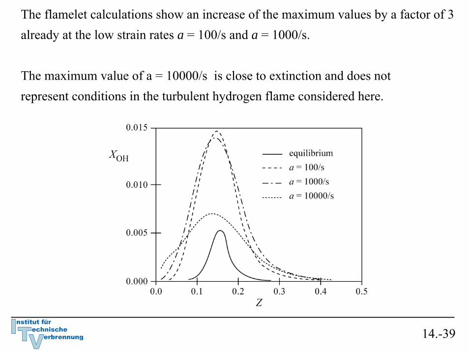
The flamelet calculations show an increase of the maximum values by a factor of 3 already at the low strain rates a = 100/s and a = 1000/s.

The maximum value of a = 10000/s is close to extinction and does notrepresent conditions in the turbulent hydrogen flame considered here.

14.-39

In summary, it may be concluded that one-point, one-time experimental data inturbulent flames, when plotted as a function of mixture fraction, showqualitatively similar tendencies as laminar flamelet profiles in counterflowdiffusion flames.

Non-equilibrium effects are evident in both cases and lead to an increaseof radical concentrations and a decrease of temperatures.

This has an important influence on NOx formation in turbulent diffusion flames.

14.-40

Laminar Flamelet Equations for Nonpremixed Combustion

Based on the laminar flamelet concept introduced in Lecture 8 the flame surface is defined as the surface of stoichiometric mixture which is obtained by setting

In the vicinity of that surface the reactive-diffusivestructure can be described by the flamelet equations

In these equations the instantaneous scalar dissipation rate has been introduced.

14.-41

At the flame surface the instantaneous scalar dissipation rate takes the value χst

If χ is assumed to be a function of Z, this functional dependence can be parameterized by χst.

The scalar dissipation rate acts as an external parameter that is imposed on the flamelet structure by the mixture fraction field.

It has the dimension of an inverse time and therefore represents the inverse of a diffusion time scale.

It also can be thought of as a diffusivity in mixture fraction space.

14.-42

In principle, both the mixture fraction Z and the scalar dissipation rate χ are fluctuating quantities and their statistical distribution needs to be considered,if one wants to calculate statistical moments of the reactive scalars (cf. Peters, (1984).

If the joint pdf surface, is known, and the steady state flameletequations are solved to obtain ψi as a function of Z and χst, point x and the time t.

The Favre mean of ψi can be obtained from

For further reading see Peters (1984).

14.-43

If the unsteady term in the flamelet equation must be retained, joint statistics of Zand χst become impractical.

Then, in order to reduce the dimension of the statistics, it is useful tointroduce multiple flamelets, each representing a different range of the χ-distribution.

Such multiple flamelets are used in the Eulerian Particle Flamelet Model (EPFM) by Barths et al. (1998).

Then the scalar dissipation rate can be formulated as a function of the mixturefraction.

14.-44

Such a formulation can be used in modeling the conditional Favre mean scalar dissipation rate

Then the flamelet equations in a turbulent flow field take the form

A mean scalar dissipation rate, however, is unable to account for those ignition and extinction events that are triggered by small and large values of χ, respectively.

This is where LES, as discussed in Lecture 10, must be used.

14.-45

With obtained from solving

Favre mean values of ψi can be obtained at any point x and time t in the flow

Here the presumed shape of the pdf can be calculated from the mean and the variance of the turbulent mixture fraction field, as discussed in Section 14.1.

14.-46

Then there remains the problem on how to model the conditional scalar dissipation rate .

One then relates the conditional scalar dissipation rate to that at a fixed value Zst by

where f(Z) is a function as in

14.-47

Then, with the presumed pdf being known, the unconditional average can be written as

Therefore, using the model

the conditional mean scalar dissipation rate can be expressed as

which is to be used in .

14.-48

Flamelet equations can also be used to describe ignition in a nonpremixed system.

As the scalar dissipation rate decreases, as for instance in a Diesel engine after injection, heat release by chemical reactions will exceed heat loss out of the reaction zone, leading to auto-ignition.

The scalar dissipation rate at auto-ignition is denoted by

For ignition under Diesel engine conditions this has been investigated byPitsch and Peters (1998).

An example of auto-ignition of a n-heptane-air mixture calculated with the RIF code (cf. Paczko et al. (1999) will be shown here.

14.-49

The initial air temperature is 1100 K and the initial fuel temperatureis 400 K.

Mixing of fuel and air leads to a straight line for theenthalpy in mixture fraction space, but not for the temperature Tu(Z), since the heat capacity cp depends on temperature.

14.-50

It is seen that auto-ignition starts after 0.203 ms, when the temperature profile shows already a smallincrease over a broad region around Z=0.2.

At t=0.218 ms there has been a fast thermal runaway in that region, with a peak at the adiabatic flame temperature.

14.-51

Turbulent combustion models have also been used to predict NOx formation inturbulent diffusion flames.

This is a problem of great practical importance, but due to the many physical aspects involved, it is also a very demanding test for any combustion model.

A very knowledgeable review on the various aspects of the problem has beengiven by Turns (1995).

A global scaling law for NO production in turbulent jet flames has been derivedby Peters and Donnerhack (1981) assuming equilibrium combustion chemistry and thin NO reaction zone around the maximum temperature in mixture fraction space.

14.-52

An asymptotic solution for the mean turbulent NO production rate can be obtained by realizing that in the expression

the function SNO(Z) has a very strong peak in the vicinity of the maximum temperature, but decreases very rapidly to both sides (shown for a hydrogen flame).

14.-53

The NO reaction rate acts nearly like a δ-function underneath the integral in

It has been shown by Peters (1978) and Janicka and Peters (1982) that an asymptotic expansion of the reaction rate around the maximum temperature leads to

where Zb is the mixture fractionat the maximum temperature Tb andSNO(Zb) is the maximum reaction rate.

14.-54

The quantity ε represents the reaction zone thickness of NO production in mixture fraction space.

That quantity was derived from the asymptotic theory as

Here ENO is the activation energy of the NO production rate.

Finally, Peters and Donnerhack (1981) predicted the NO emission index EINO, which represents the total mass flow rate of NO produced per mass flow rate of fuel, as being proportional to

14.-55

In

L is the flame length, d the nozzle diameter and u0 the jet exit velocity.

The normalized flame length L/d is constant for momentum dominated jets but scales with the Froude number Fr=u0

2/(gd) as L/d ~ Fr1/5

for buoyancy dominated jets as shown in the figure.

14.-56

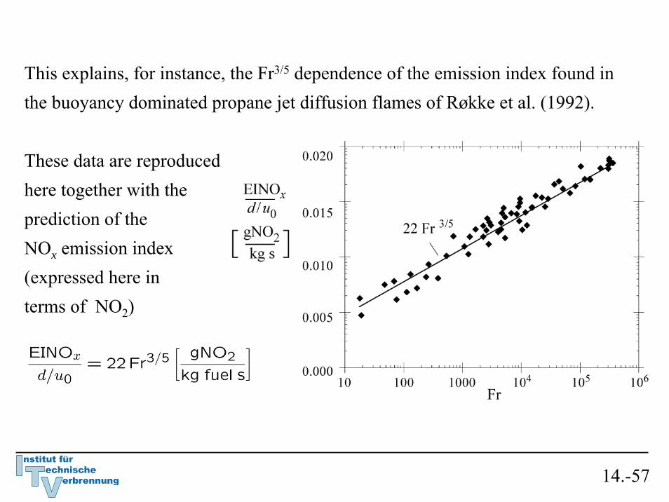
This explains, for instance, the Fr3/5 dependence of the emission index found in the buoyancy dominated propane jet diffusion flames of Røkke et al. (1992).

These data are reproduced here together with the prediction of the NOx emission index(expressed here in terms of NO2)

14.-57

An interesting set of experimental data are those by Chen and Driscoll(1990) and Driscoll et al. (1992) for diluted hydrogen flames.

These data show a square root dependence of them rescaled emission index on the Damköhler number.

An explanation for this scaling may be found by using the steady state flameletequation for the second derivative of temperature in

rather than the equilibrium profile.

14.-58

This may be written as

Here the term on the r.h.s., evaluated at and divided by the maximum temperature, may also be interpreted as a Damköhler number.

Inserting this into

the quantity ε becomes proportional to Da-1/2.

14.-59

This finally leads with

to

This scaling law indicates that the experimentally observed (d/u0)1/2 dependence of the rescaled NO emission index is a residence time effect, modified by the temperature sensitivity of the NO reaction rate, on which the asymptotic theory by Peters and Donnerhack (1981) was built.

It also shows that unsteady effects of the flame structure and super-equilibrium O-concentrations may be of less importance than is generally assumed.

14.-60

Appendix

A

As in

and

the transport term containing the molecular diffusivity has been neglected

as being small compared to the turbulent transport term. Effects due to non-unity Lewis numbers have also been neglected.

14.-10

No equation for enthalpy fluctuations is presented here, because in nonpremixed turbulent combustion, it is often assumed that fluctuations of the enthalpy are mainly due to mixture fraction fluctuations and are described by those.

14.-10

If the assumption of fast chemistry is introduced and the coupling between themixture fraction and the enthalpy

can be used, the Burke-Schumann solution or the equilibrium solution relatesall reactive scalars to the local mixture fraction.

Using these relations the easiest way to obtain mean values of the reactive scalars is to use the presumed shape pdf approach.

This is called the Conserved Scalar Equilibrium Model.

14.-13

For such shapes, which have been found in jets and shear layers, a compositemodel has been developed by Effelsberg and Peters (1983).

It identifies three different contributions to the pdf:

1) a fully turbulent part, 2) an outer flow part and 3) a part which was related to the viscous superlayer between the outer flow and the fully turbulent flow region.

The model shows that the intermediate maximum is due to the contribution from the fully turbulent part of the scalar field.

14.-18

The overall agreement between the experimental data and the equilibriumsolution is quite good.

This is often observed for hydrogen flames where chemistry is typically very fast.

On the contrary, hydrocarbon flames at high exit velocities and small nozzle diameters are likely to exhibit local extinction and non-equilibrium effects,discussed in Masri et al. (1996).

14.-43

The equation

shows that ψi depends on the mixture fraction Z, on the scalar dissipation rate χ, and on time t.

This implies that the reactive scalars are constant along iso-mixture fraction surfaces at a given time and a prescribed functional form of the scalar dissipation rate.

Thereby the fields of the reactive scalars are aligned to that of the mixture fraction and are transported together with it by the flow field.

14.-50

Flamelet equations can also be used to describe ignition in a nonpremixedsystem.

If fuel and oxidizer are initially at the unburnt temperature Tu(Z), asshown in the figure, but the scalar dissipation rate is still large enough, so that heat loss out of the reaction zone exceeds the Heat release by chemical reactions, a thermal runaway is not possible.

This corresponds to the steady state lower branch in the S-shaped curve.

14.-57

From thereon, the temperature profile broadens, which may be interpreted as a propagation of two fronts in mixture fraction space, one towards the lean and the other towards the rich mixture.

Although the transport termin

contributes to this propagation,it should be kept in mind that themixture is close to auto-ignition everywhere.

The propagation of an ignition front in mixture fraction space therefore differs considerably from premixed flame propagation.

14.-61

At t = 0.3 ms most of the mixture, except for a region beyond Z = 0.4 inmixture fraction space, has reached the equilibrium temperature.

A maximum value of T = 2750 K is found close to stoichiometric mixture.

The ignition of n-heptanemixtures under Diesel engine condition has been discussed in detail by Pitsch and Peters (1998).

There it is shown that auto-ignition under nonpremixed conditions occurs mainly at locations in a turbulent flow field where the scalar dissipation rate is low.

14.-62

It is interesting to note that by taking the values SNO(Zb)=10.8 . 10-3/s and ε=0.109 for propane from Peters and Donnerhack (1981) and using

in the buoyancy dominated limit one calculates a factor of 27.2 rather than 22 in

Since Peters and Donnerhack (1981) had assumed equilibrium combustion chemistry, the second derivative of the temperature in

was calculated from an equilibrium temperature profile.

14.-69

Therefore ε was tabulated as a constant for each fuel

If the quantity SNO(Zb)d/u0 is interpreted as a Damköhler number the rescaled emission index from

is

proportional to that Damköhler number.

14.-70

Sanders et al. (1997) have reexamined steady state flamelet modeling using the two variable presumed shape pdf model for the mixture fractions and, either the scalar dissipation rate or the strain rate as second variable.

Their study revealed that only the formulation using the scalar dissipation rate asthe second variable was able to predict the Da1/2 dependence of the data ofDriscoll et al. (1992).

This is in agreement with results of Ferreira (1996).

14.-74

In addition Sanders et al. (1997) examined whether there is a difference between using a lognormal pdf of χst with a variance of unity and a delta function pdf and found that both assumptions gave similar results.

Their predictions improved with increasing Damköhler number and their results also suggest that Lei = 1 is the best choice for these hydrogen flames.

14.-75

For a turbulent jet flame with a fuel mixture of 31 % methane and 69 % hydrogen Chen and Chang (1996) performed a detailed comparison between steady state flamelet and pdf modeling.

They found that radiative heat loss becomes increasingly important for NO predictions further downstream in the flame.

This is in agreement with the comparison of time scales by Pitsch et al. (1998) who found that radiation is too slow to be effective as far as the combustion reactions are concerned, but that it effects NO levels considerably.

14.-76