Lecture 12 Simplex method - Engineeringseas.ucla.edu/~vandenbe/ee236a/lectures/simplex.pdf ·...

L. Vandenberghe EE236A (Fall 2013-14)

Lecture 12Simplex method

• adjacent extreme points

• one simplex iteration

• cycling

• initialization

• implementation

12–1

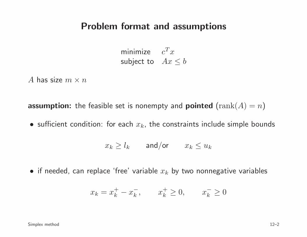
Problem format and assumptions

minimize cTxsubject to Ax ≤ b

A has size m× n

assumption: the feasible set is nonempty and pointed (rank(A) = n)

• sufficient condition: for each xk, the constraints include simple bounds

xk ≥ lk and/or xk ≤ uk

• if needed, can replace ‘free’ variable xk by two nonnegative variables

xk = x+k − x−

k , x+k ≥ 0, x−

k ≥ 0

Simplex method 12–2

Simplex method

• invented in 1947 (George Dantzig)

• usually developed for LPs in standard form (‘primal’ simplex method)

• we will outline the ‘dual’ simplex method (for inequality form LP)

one iteration:

move from an extreme point to an adjacent extreme point with lower cost

questions

1. how are extreme points characterized? (see lecture 3)

2. how do we find an adjacent extreme point with lower cost?

3. when does the iteration terminate?

4. how do we find an initial extreme point?


Extreme points

recall rank test: to check whether x is an extreme point of solution set of

aTi x ≤ bi, i = 1, . . . ,m

• check that x satisfies the inequalities

• find the active constraints at x,

J = {i1, . . . , ik} = {i | aTi x = bi},

and define the submatrix

AJ =

aTi1aTi2...aTik

• x is an extreme point if and only if rank(AJ) = n


Degeneracy

extreme point x is nondegenerate if exactly n inequalities are active at it

• AJ is square (|J | = n) and nonsingular

• therefore x can be written as x = A−1J bJ , where bJ = (bi1, bi2, . . . , bin)

an extreme point is degenerate if more than n inequalities are active at x

note:

• extremality is a geometric property (of the set P = {x | Ax ≤ b})

• (non-)degeneracy also depends on the description of P (i.e., A and b)

until p. 12–20 we assume that all extreme points of P are nondegenerate


Adjacent extreme points

definition:

extreme points are adjacent if they have n− 1 common active constraints

example

0 −1−1 −1−1 0−1 1

[

x1

x2

]≤

0−102

(1, 0)

(0, 1)

(0, 2)

x b−Ax J(1, 0) (0, 0, 1, 3) {1, 2}(0, 1) (1, 0, 0, 1) {2, 3}(0, 2) (2, 1, 0, 0) {3, 4}


Moving to an adjacent extreme point

given: extreme point x with active index set J , and an index k ∈ J

problem: find adjacent extreme point x with active set containing J \ {k}

1. solve the set of n equations in n variables

aTi ∆x = 0, i ∈ J \ {k}, aTk∆x = −1

2. if A∆x ≤ 0, then {x+ α∆x | α ≥ 0} is a feasible half-line:

A(x+ α∆x) ≤ b ∀α ≥ 0

3. else, take x = x+ α∆x where α = max{α | A(x+ α∆x) ≤ b}, i.e.,

α = mini:aT

i∆x>0

bi − aTi x

aTi ∆x


discussion

• equations in step 1 are solvable because AJ is nonsingular

• α computed in step 3 is positive: AJ∆x ≤ 0 by construction, so

aTi ∆x > 0 =⇒ i 6∈ J =⇒ aTi x < bi

• x = x+ α∆x is feasible with active constraints J = (J \ {k})∪ I, where

I = {i | aTi ∆x > 0,bi − aTi x

aTi ∆x= α}

• x is an extreme point (rank(AJ) = n): take any j ∈ I; since

aTj ∆x > 0, aTi ∆x = 0 for i ∈ J \ {k}

the vector aj is linearly independent of the vectors ai, i ∈ J \ {k}

• by nondegeneracy assumption, |I| = 1 (minimizer in step 3 is unique)


Example

find the extreme points adjacent to x = (1, 0) (for example on p. 12–6)

1. try to remove k = 1 from active set J = {1, 2}

• compute ∆x

[0 −1

−1 −1

] [∆x1

∆x2

]=

[−10

]=⇒ ∆x = (−1, 1)

• minimum ratio test: A∆x = (−1, 0, 1, 2)

α = min{b3 − aT3 x

aT3∆x,b4 − aT4 x

aT4∆x} = min{

1

1,3

2} = 1

new extreme point: x = (0, 1) with active set J = {2, 3}


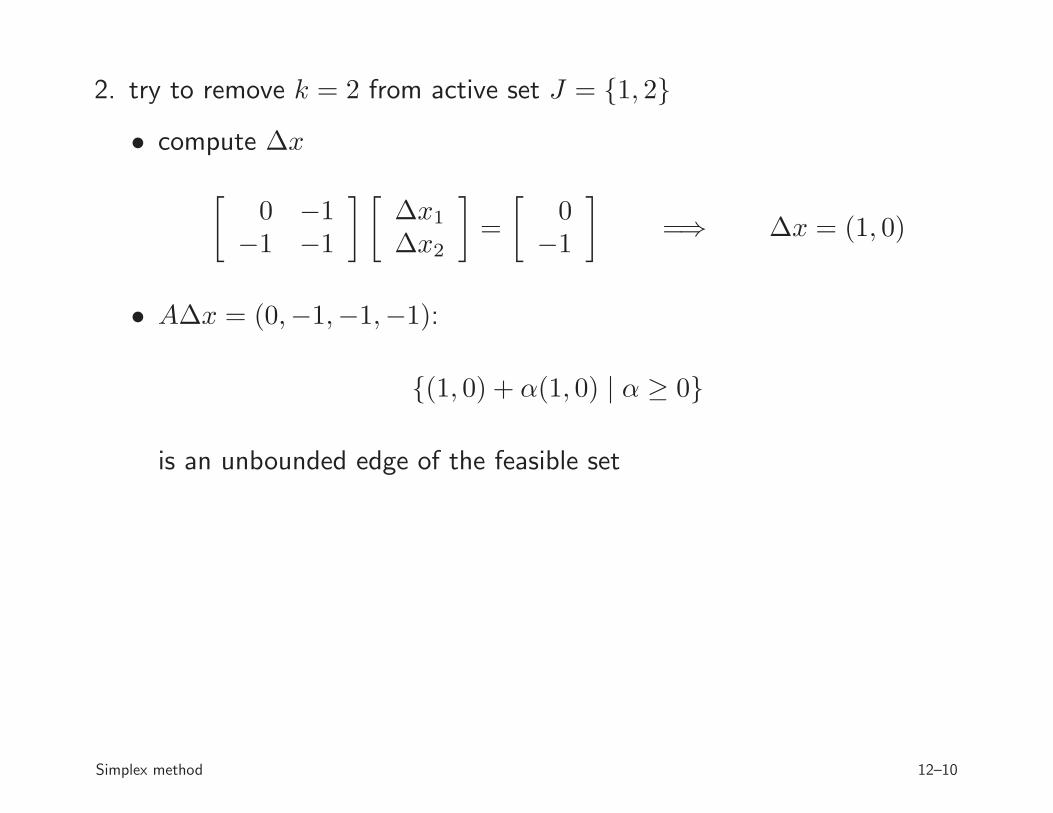
2. try to remove k = 2 from active set J = {1, 2}

• compute ∆x

[0 −1

−1 −1

] [∆x1

∆x2

]=

[0

−1

]=⇒ ∆x = (1, 0)

• A∆x = (0,−1,−1,−1):

{(1, 0) + α(1, 0) | α ≥ 0}

is an unbounded edge of the feasible set


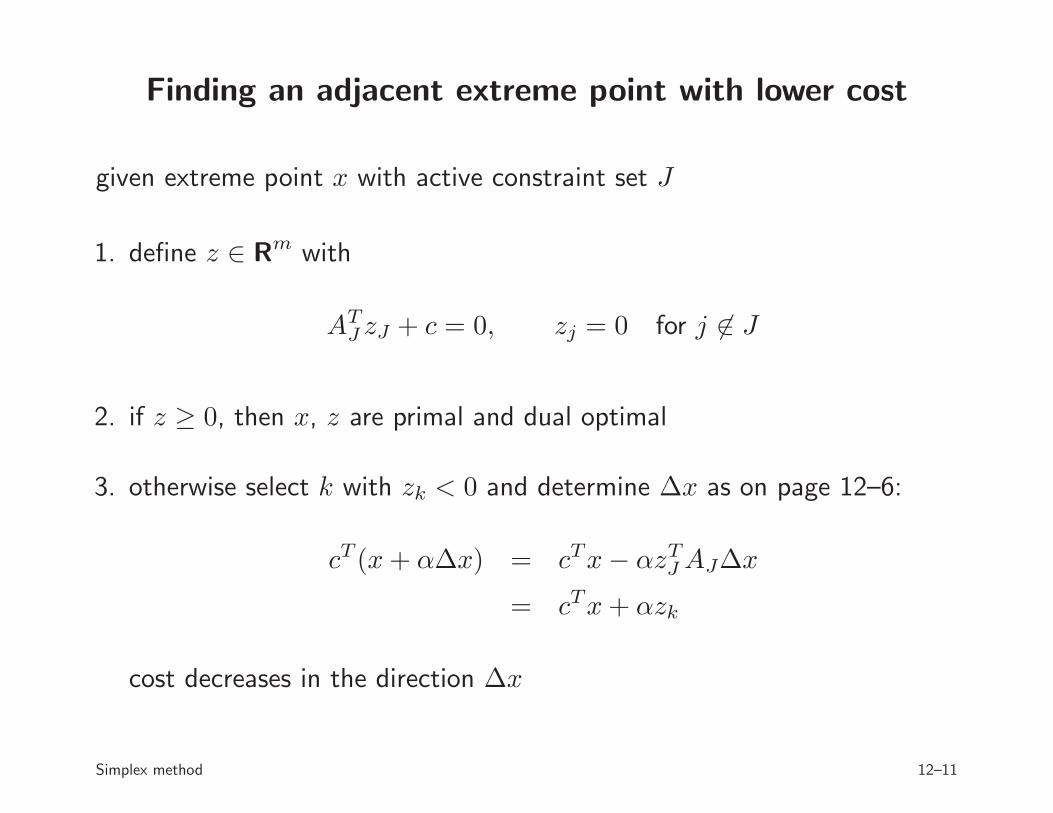
Finding an adjacent extreme point with lower cost

given extreme point x with active constraint set J

1. define z ∈ Rm with

ATJ zJ + c = 0, zj = 0 for j 6∈ J

2. if z ≥ 0, then x, z are primal and dual optimal

3. otherwise select k with zk < 0 and determine ∆x as on page 12–6:

cT (x+ α∆x) = cTx− αzTJAJ∆x

= cTx+ αzk

cost decreases in the direction ∆x


One iteration of the simplex method

given an extreme point x with active set J

1. compute z ∈ Rm with

ATJ zJ + c = 0, zj = 0 for j 6∈ J

if z ≥ 0, terminate: x, z are primal, dual optimal

2. choose k with zk < 0 and compute ∆x ∈ Rn with

aTi ∆x = 0 for i ∈ J \ {k}, aTk∆x = −1

if A∆x ≤ 0, terminate: LP is unbounded (p⋆ = −∞)

3. set J := J \ {k} ∪ {j} and x := x+ α∆x where

j = argmini:aT

i∆x>0

bi − aTi x

aTi ∆x, α =

bj − aTj x

aTj ∆x


Pivot selection and convergence

step 2: which k do we choose if zk has several negative components?

many variants:

• choose most negative zk

• choose maximum decrease in cost αzk

• choose smallest k

all three variants work (if extreme points are nondegenerate)

step 3: j is unique and α > 0 (if all extreme points are nondegenerate)

convergence follows from:

• finiteness of number of extreme points

• strict decrease in cost function at each step


Example

min. x1 + x2 − x3 s.t.

−1 0 00 −1 00 0 −11 0 00 1 00 0 11 1 1

x1

x2

x3

≤

0002225

��

��

(2, 0, 0)

(2, 0, 2)

(0, 0, 2) (0, 2, 2)

(0, 2, 0)

(2, 2, 0)

(0, 0, 0)(2, 2, 1)

(2, 1, 2)

(1, 2, 2)

• optimal point is x = (0, 0, 2)

• start simplex method at x = (2, 2, 0)


iteration 1: x = (2, 2, 0), b−Ax = (2, 2, 0, 0, 0, 2, 1), J = {3, 4, 5}

1. compute z:

0 1 00 0 1

−1 0 0

z3z4z5

= −

11

−1

=⇒ z = (0, 0,−1,−1,−1, 0, 0)

not optimal; remove k = 3 from active set

2. compute ∆x

0 0 −11 0 00 1 0

∆x1

∆x2

∆x3

=

−100

=⇒ ∆x = (0, 0, 1)

3. minimum ratio test: A∆x = (0, 0,−1, 0, 0, 1, 1)

α = argmin{2/1, 1/1} = 1, j = 7


iteration 2: x = (2, 2, 1), b−Ax = (2, 2, 1, 0, 0, 1, 0), J = {4, 5, 7}

1. compute z:

1 0 10 1 10 0 1

z4z5z7

= −

11

−1

=⇒ z = (0, 0, 0,−2,−2, 0, 1)


2. compute ∆x

1 0 00 1 01 1 1

∆x1

∆x2

∆x3

=

0−10

=⇒ ∆x = (0,−1, 1)

3. minimum ratio test: A∆x = (0, 1,−1, 0,−1, 1, 0)

α = argmin{2/1, 1/1} = 1, j = 6


iteration 3: x = (2, 1, 2), b−Ax = (2, 1, 2, 0, 1, 0, 0), J = {4, 6, 7}

1. compute z:

1 0 10 0 10 1 1

z4z6z7

= −

11

−1

=⇒ z = (0, 0, 0, 0, 0, 2,−1)


2. compute ∆x

1 0 00 0 11 1 1

∆x1

∆x2

∆x3

=

00

−1

=⇒ ∆x = (0,−1, 0)

3. minimum ratio test: A∆x = (0, 1, 0, 0,−1, 0,−1)

α = argmin{1/1} = 1, j = 2


iteration 4: x = (2, 0, 2), b−Ax = (2, 0, 2, 0, 2, 0, 1), J = {2, 4, 6}

1. compute z:

0 1 0−1 0 00 0 1

z2z4z6

= −

11

−1

=⇒ z = (0, 1, 0,−1, 0, 1, 0)


2. compute ∆x

0 −1 01 0 00 0 1

∆x1

∆x2

∆x3

=

0−10

=⇒ ∆x = (−1, 0, 0)

3. minimum ratio test: A∆x = (1, 0, 0,−1, 0, 0,−1)

α = argmin{2/1} = 2, j = 1


iteration 5: x = (0, 0, 2), b−Ax = (0, 0, 2, 2, 2, 0, 3), J = {1, 2, 6}

1. compute z:

−1 0 00 −1 00 0 1

z1z2z6

= −

11

−1

=⇒ z = (1, 1, 0, 0, 0, 1, 0)

optimal


Degeneracy

• if x is degenerate, AJ has rank n but is not square

• if next point is degenerate, we have a tie in the minimization in step 3

solution

• define J to be a subset of n linearly independent active constraints

• AJ is square; steps 1 and 2 work as in the nondegenerate case

• in step 3, break ties arbitrarily

does it work?

• in step 3 we can have α = 0 (i.e., x does not change)

• maybe this is okay, as long as J keeps changing


Example

minimize −3x1 + 5x2 − x3 + 2x4

subject to

1 −2 −2 32 −3 −1 10 0 1 0

−1 0 0 00 −1 0 00 0 −1 00 0 0 −1

x1

x2

x3

x4

≤

0010000

• x = (0, 0, 0, 0) is a degenerate extreme point with

b−Ax = (0, 0, 1, 0, 0, 0, 0)

• start simplex with J = {4, 5, 6, 7}


iteration 1: J = {4, 5, 6, 7}

1. z = (0, 0, 0,−3, 5,−1, 2): remove 4 from active set

2. ∆x = (1, 0, 0, 0)

3. A∆x = (1, 2, 0,−1, 0, 0, 0): α = 0, add 1 to active set

iteration 2: J = {1, 5, 6, 7}

1. z = (3, 0, 0, 0,−1,−7, 11): remove 5 from active set

2. ∆x = (2, 1, 0, 0)

3. A∆x = (0, 1, 0,−2,−1, 0, 0): α = 0, add 2 to active set

iteration 3: J = {1, 2, 6, 7}

1. z = (1, 1, 0, 0, 0,−4, 6): remove 6 from active set

2. ∆x = (−4,−3, 1, 0)

3. A∆x = (0, 0, 1, 4, 3,−1, 0): α = 0, add 4 to active set


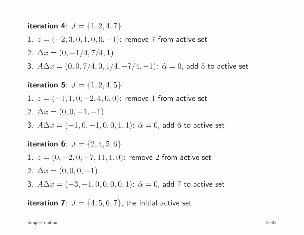
iteration 4: J = {1, 2, 4, 7}

1. z = (−2, 3, 0, 1, 0, 0,−1): remove 7 from active set

2. ∆x = (0,−1/4, 7/4, 1)

3. A∆x = (0, 0, 7/4, 0, 1/4,−7/4,−1): α = 0, add 5 to active set

iteration 5: J = {1, 2, 4, 5}

1. z = (−1, 1, 0,−2, 4, 0, 0): remove 1 from active set

2. ∆x = (0, 0,−1,−1)

3. A∆x = (−1, 0,−1, 0, 0, 1, 1): α = 0, add 6 to active set

iteration 6: J = {2, 4, 5, 6}

1. z = (0,−2, 0,−7, 11, 1, 0): remove 2 from active set

2. ∆x = (0, 0, 0,−1)

3. A∆x = (−3,−1, 0, 0, 0, 0, 1): α = 0, add 7 to active set

iteration 7: J = {4, 5, 6, 7}, the initial active set


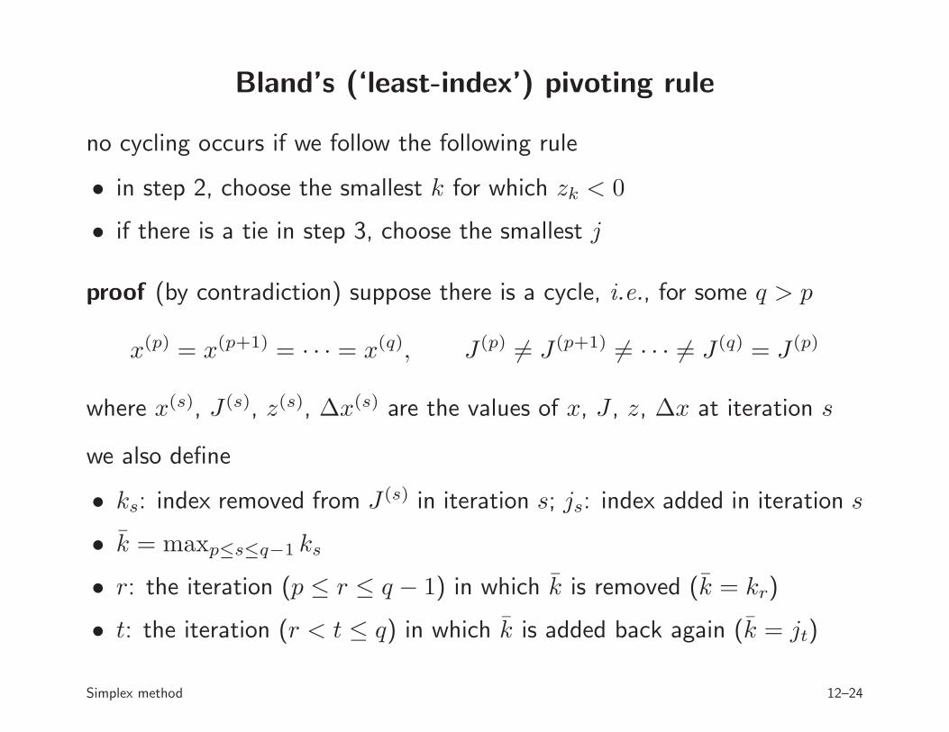
Bland’s (‘least-index’) pivoting rule

no cycling occurs if we follow the following rule

• in step 2, choose the smallest k for which zk < 0

• if there is a tie in step 3, choose the smallest j

proof (by contradiction) suppose there is a cycle, i.e., for some q > p

x(p) = x(p+1) = · · · = x(q), J (p) 6= J (p+1) 6= · · · 6= J (q) = J (p)

where x(s), J (s), z(s), ∆x(s) are the values of x, J , z, ∆x at iteration s

we also define

• ks: index removed from J (s) in iteration s; js: index added in iteration s

• k = maxp≤s≤q−1 ks

• r: the iteration (p ≤ r ≤ q − 1) in which k is removed (k = kr)

• t: the iteration (r < t ≤ q) in which k is added back again (k = jt)


at iteration r we remove index k from J (r); therefore

• z(r)

k< 0

• z(r)i ≥ 0 for i ∈ J (r), i < k (otherwise we should have removed i)

• z(r)i = 0 for i 6∈ J (r) (by definition of z(r))

at iteration t we add index k to J (t); therefore

• aTk∆x(t) > 0

• aTi ∆x(t) ≤ 0 for i ∈ J (r), i < k

(otherwise we should have added i, since bi − aTi x = 0 for all i ∈ J (r))

• aTi ∆x(t) = 0 for i ∈ J (r), i > k

(if i > k and i ∈ J (r) then it is never removed, so i ∈ J (t) \ {kt})

conclusion: z(r)TA∆x(t) < 0

a contradiction, because −z(r)TA∆x(t) = cT∆x(t) ≤ 0


Example

example of page 12–21, same starting point but applying Bland’s rule

iteration 1: J = {4, 5, 6, 7}

1. z = (0, 0, 0,−3, 5,−1, 2): remove 4 from active set

2. ∆x = (1, 0, 0, 0)

3. A∆x = (1, 2, 0,−1, 0, 0, 0): α = 0, add 1 to active set

iteration 2: J = {1, 5, 6, 7}

1. z = (3, 0, 0, 0,−1,−7, 11): remove 5 from active set

2. ∆x = (2, 1, 0, 0)



iteration 3: J = {1, 2, 6, 7}

1. z = (1, 1, 0, 0, 0,−4, 6): remove 6 from active set

2. ∆x = (−4,−3, 1, 0)

3. A∆x = (0, 0, 1, 4, 3,−1, 0): α = 0, add 4 to active set

iteration 4: J = {1, 2, 4, 7}

1. z = (−2, 3, 0, 1, 0, 0,−1): remove 1 from active set

2. ∆x = (0,−1/4, 3/4, 1)

3. A∆x = (−1, 0, 3/4, 0, 1/4,−3/4, 0): α = 0, add 5 to active set

iteration 5: J = {2, 4, 5, 7}

1. z = (0,−1, 0,−5, 8, 0, 1): remove 2 from active set

2. ∆x = (0, 0, 1, 0)

3. A∆x = (−2,−1, 1, 0, 0,−1, 0): α = 1, add 3 to active set

new x = (0, 0, 1, 0), b−Ax = (2, 1, 0, 0, 0, 1, 0)


iteration 6: J = {3, 4, 5, 7}

1. z = (0, 0, 1,−3, 5, 0, 2): remove 4 from active set

2. ∆x = (1, 0, 0, 0)

3. A∆x = (1, 2, 0,−1, 0, 0, 0): α = 1/2, add 2 to active set

new x = (1/2, 0, 1, 0), b−Ax = (3/2, 0, 0, 1/2, 0, 1, 0)

iteration 7: J = {1, 3, 5, 7}

1. z = (3, 0, 7, 0,−1, 0, 11): remove 5 from active set

2. ∆x = (2, 1, 0, 0)


iteration 8: J = {1, 2, 3, 7}

1. z = (1, 1, 4, 0, 0, 0, 6): optimal


Initialization

linear program with variable bounds

minimize cTxsubject to Ax ≤ b, x ≥ 0

(general: free xk can be split as xk = x+k − x−

k with x+k ≥ 0, x−

k ≥ 0)

phase I problem

minimize tsubject to Ax ≤ (1− t)b, x ≥ 0, 0 ≤ t ≤ 1

• x = 0, t = 1 is an extreme point for phase I problem

• can compute an optimal extreme point x⋆, t⋆ via simplex method

• if t⋆ > 0, original problem is infeasible

• if t⋆ = 0, then x⋆ is an extreme point of original problem


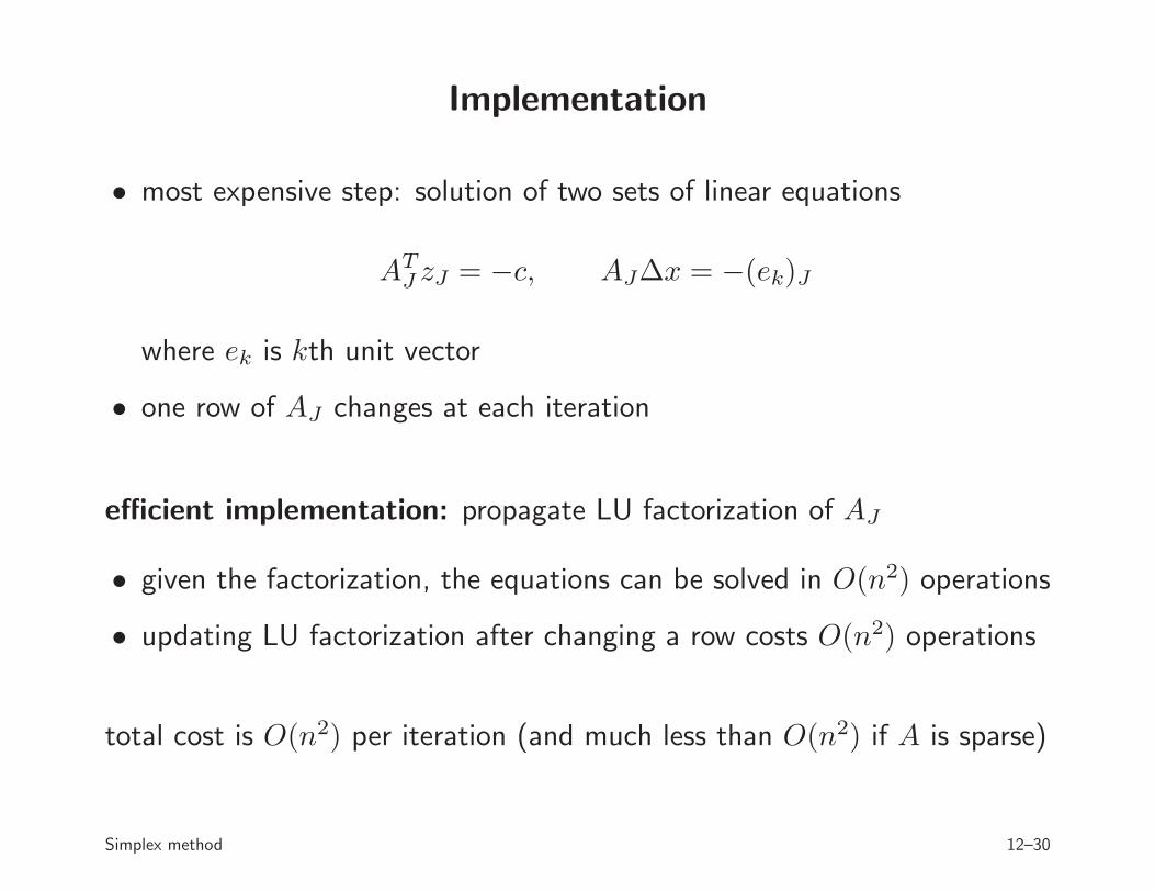
Implementation

• most expensive step: solution of two sets of linear equations

ATJ zJ = −c, AJ∆x = −(ek)J

where ek is kth unit vector

• one row of AJ changes at each iteration

efficient implementation: propagate LU factorization of AJ

• given the factorization, the equations can be solved in O(n2) operations

• updating LU factorization after changing a row costs O(n2) operations

total cost is O(n2) per iteration (and much less than O(n2) if A is sparse)


Complexity

worst-case

• for most pivoting rules, there exist examples where the number ofiterations grows exponentially with n and m

• it is an open question whether there exists a pivoting rule for which thenumber of iterations is bounded by a polynomial of n and m

in practice: very efficient (#iterations typically grows linearly with m, n)


Lecture 12 Simplex method - Engineeringseas.ucla.edu/~vandenbe/ee236a/lectures/simplex.pdf ·...

Documents

Transcript of Lecture 12 Simplex method - Engineeringseas.ucla.edu/~vandenbe/ee236a/lectures/simplex.pdf ·...