Lecture 12: more Chapter 5, Section 3 Relationships...

©2011 Brooks/Cole, CengageLearning

Elementary Statistics: Looking at the Big Picture 1

Lecture 12: more Chapter 5, Section 3Relationships between TwoQuantitative Variables; RegressionEquation of Regression Line; ResidualsEffect of Explanatory/Response RolesUnusual ObservationsSample vs. PopulationTime Series; Additional Variables

©2011 Brooks/Cole,Cengage Learning

Elementary Statistics: Looking at the Big Picture L12.2

Looking Back: Review

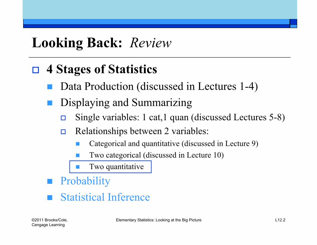
4 Stages of Statistics Data Production (discussed in Lectures 1-4) Displaying and Summarizing

Single variables: 1 cat,1 quan (discussed Lectures 5-8) Relationships between 2 variables:

Categorical and quantitative (discussed in Lecture 9) Two categorical (discussed in Lecture 10) Two quantitative

Probability Statistical Inference



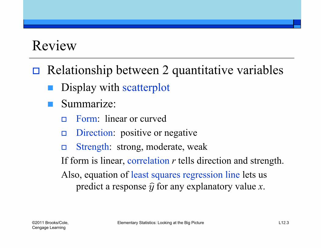
Review Relationship between 2 quantitative variables

Display with scatterplot Summarize:

Form: linear or curved Direction: positive or negative Strength: strong, moderate, weakIf form is linear, correlation r tells direction and strength.Also, equation of least squares regression line lets us

predict a response for any explanatory value x.



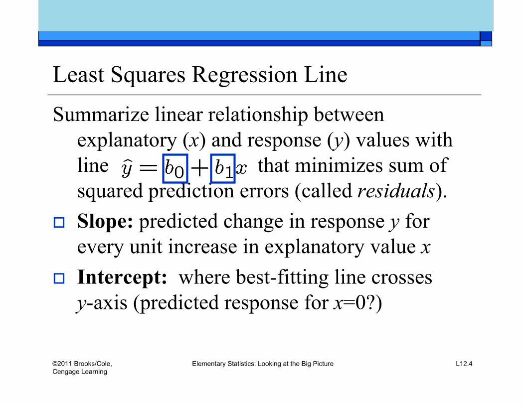
Least Squares Regression LineSummarize linear relationship between

explanatory (x) and response (y) values withline that minimizes sum ofsquared prediction errors (called residuals).

Slope: predicted change in response y forevery unit increase in explanatory value x

Intercept: where best-fitting line crossesy-axis (predicted response for x=0?)



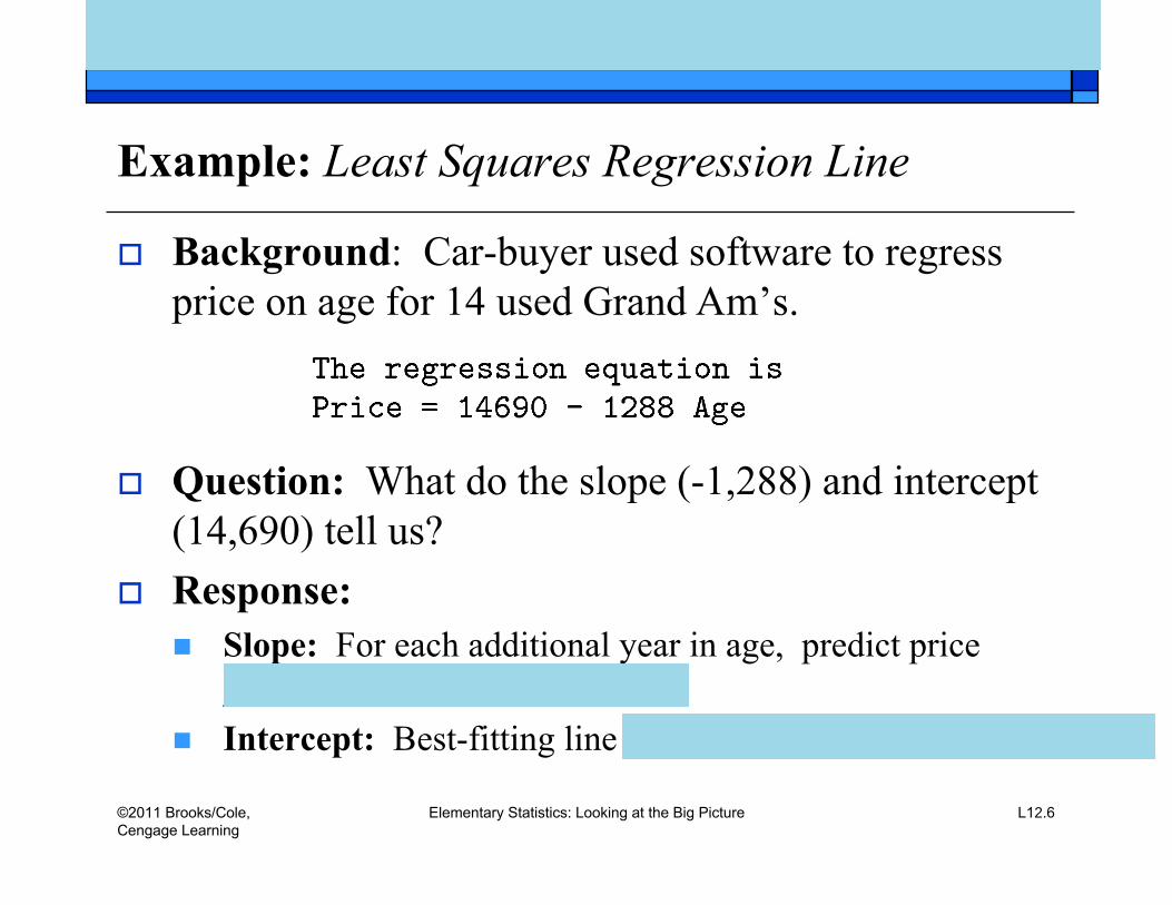
Example: Least Squares Regression Line

Background: Car-buyer used software to regressprice on age for 14 used Grand Am’s.

Question: What do the slope (-1,288) and intercept(14,690) tell us?

Response: Slope: For each additional year in age, predict price

___________________ Intercept: Best-fitting line ________________________

nancyp

Text Box

Practice: 5.70f p.203



Example: Extrapolation

Background: Car-buyer used software to regressprice on age for 14 used Grand Am’s.

Question: Should we predict a new Grand Am tocost $14,690-$1,288(0)=$14,690?

Response:

nancyp

Text Box

Practice: 5.54c p.197



Definition Extrapolation: using the regression line to

predict responses for explanatory valuesoutside the range of those used to constructthe line.



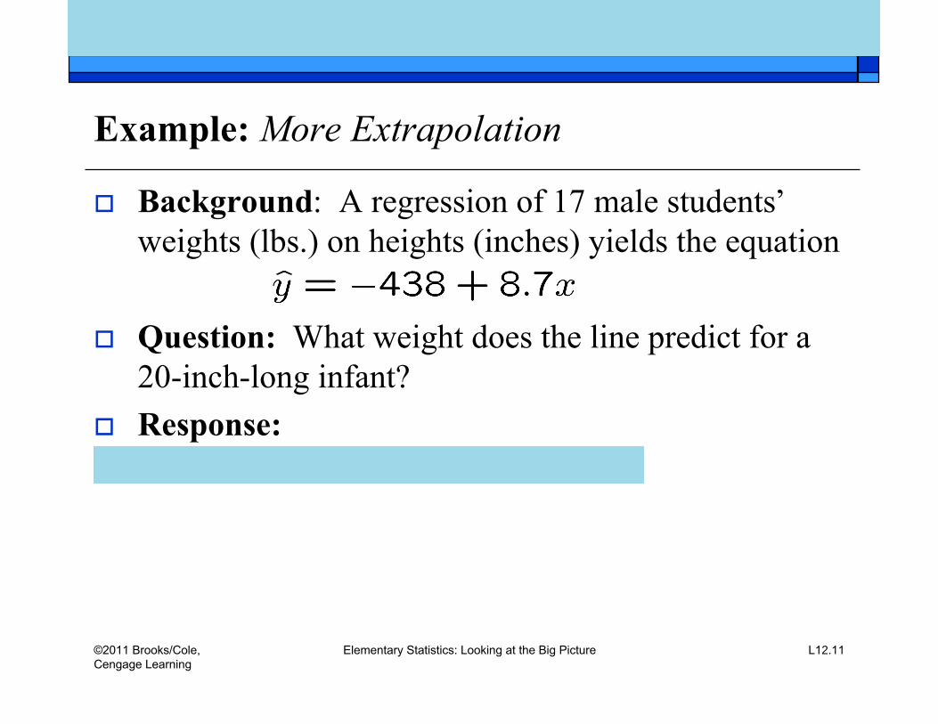
Example: More Extrapolation

Background: A regression of 17 male students’weights (lbs.) on heights (inches) yields the equation

Question: What weight does the line predict for a20-inch-long infant?

Response:

nancyp

Text Box

Practice: 5.36e p.193



Expressions for slope and interceptConsider slope and intercept of the least squares

regression line Slope: so if x increases by a

standard deviation, predict y to increase by rstandard deviations

Intercept: so whenpredict

the line passes through the point of averages



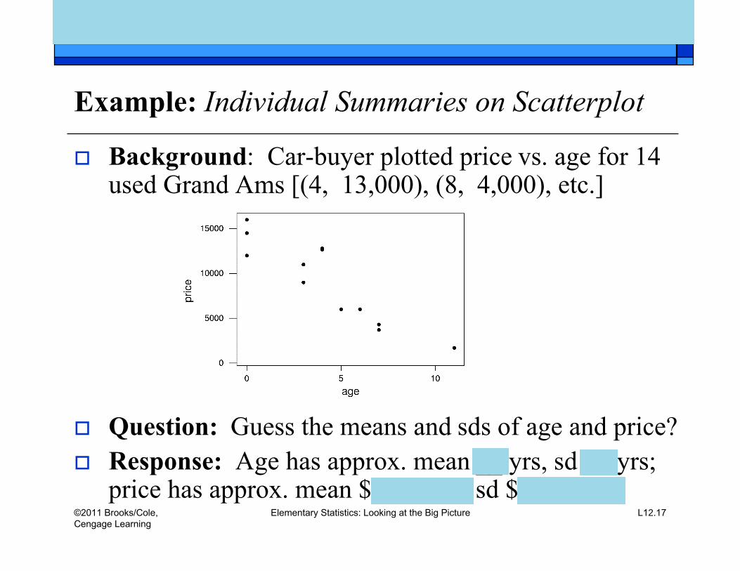
Example: Individual Summaries on Scatterplot

Background: Car-buyer plotted price vs. age for 14used Grand Ams [(4, 13,000), (8, 4,000), etc.]

Question: Guess the means and sds of age and price? Response: Age has approx. mean __ yrs, sd __ yrs;

price has approx. mean $_______, sd $_______.

nancyp

Text Box

Practice: 5.50a-d p.196



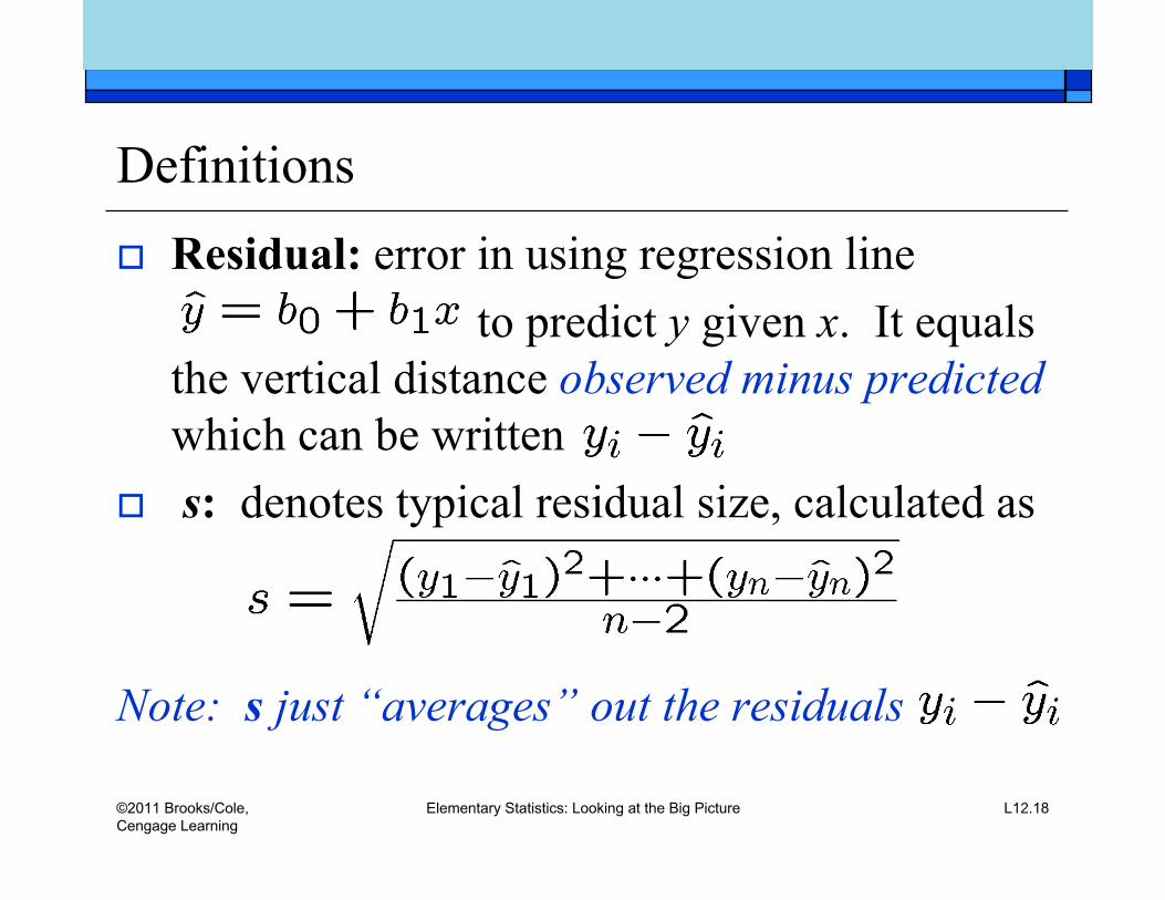
Definitions Residual: error in using regression line

to predict y given x. It equalsthe vertical distance observed minus predictedwhich can be written

s: denotes typical residual size, calculated as

Note: s just “averages” out the residuals



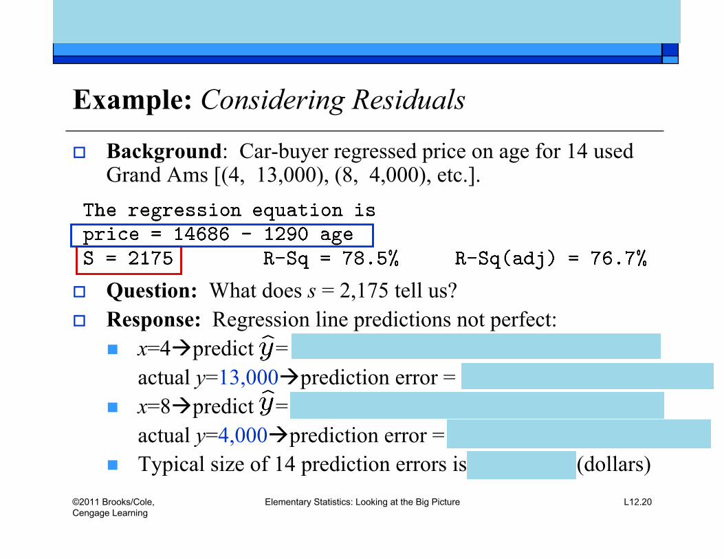
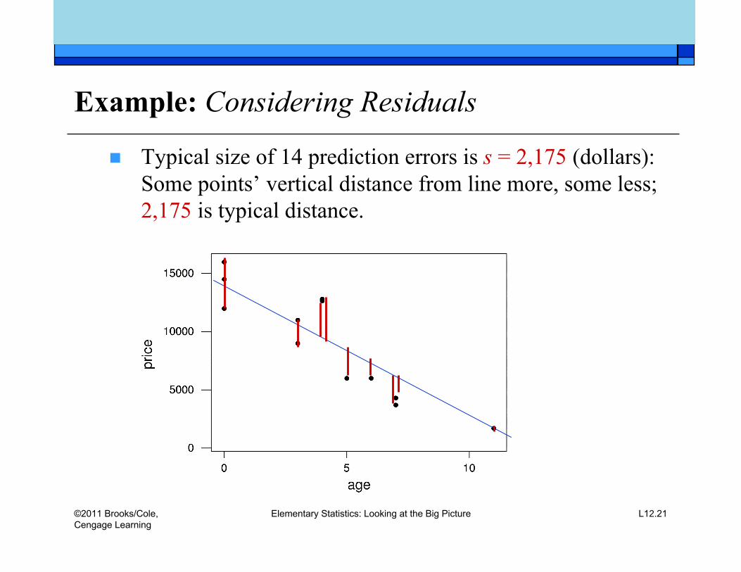
Example: Considering Residuals

Background: Car-buyer regressed price on age for 14 usedGrand Ams [(4, 13,000), (8, 4,000), etc.].

Question: What does s = 2,175 tell us? Response: Regression line predictions not perfect:

x=4predict =actual y=13,000prediction error =

x=8predict =actual y=4,000prediction error =

Typical size of 14 prediction errors is _________ (dollars)

nancyp

Text Box

Practice: 5.56a p.197



Example: Considering Residuals

Typical size of 14 prediction errors is s = 2,175 (dollars):Some points’ vertical distance from line more, some less;2,175 is typical distance.



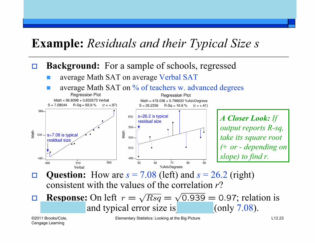
Example: Residuals and their Typical Size s

Background: For a sample of schools, regressed average Math SAT on average Verbal SAT average Math SAT on % of teachers w. advanced degrees

Question: How are s = 7.08 (left) and s = 26.2 (right)consistent with the values of the correlation r?

Response: On left ; relation is________ and typical error size is________(only 7.08).

A Closer Look: Ifoutput reports R-sq,take its square root(+ or - depending onslope) to find r.

nancyp

Text Box

Practice: 5.70i-k p.203



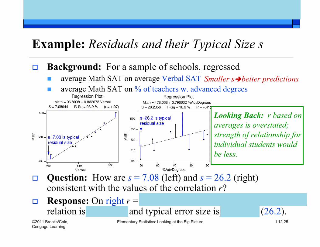
Example: Residuals and their Typical Size s

Background: For a sample of schools, regressed average Math SAT on average Verbal SAT average Math SAT on % of teachers w. advanced degrees

Question: How are s = 7.08 (left) and s = 26.2 (right)consistent with the values of the correlation r?

Response: On right r = _____________________________;relation is ________ and typical error size is________ (26.2).

Looking Back: r based onaverages is overstated;strength of relationship forindividual students wouldbe less.

Smaller sbetter predictions

nancyp

Text Box

Practice: 5.70i-k p.203



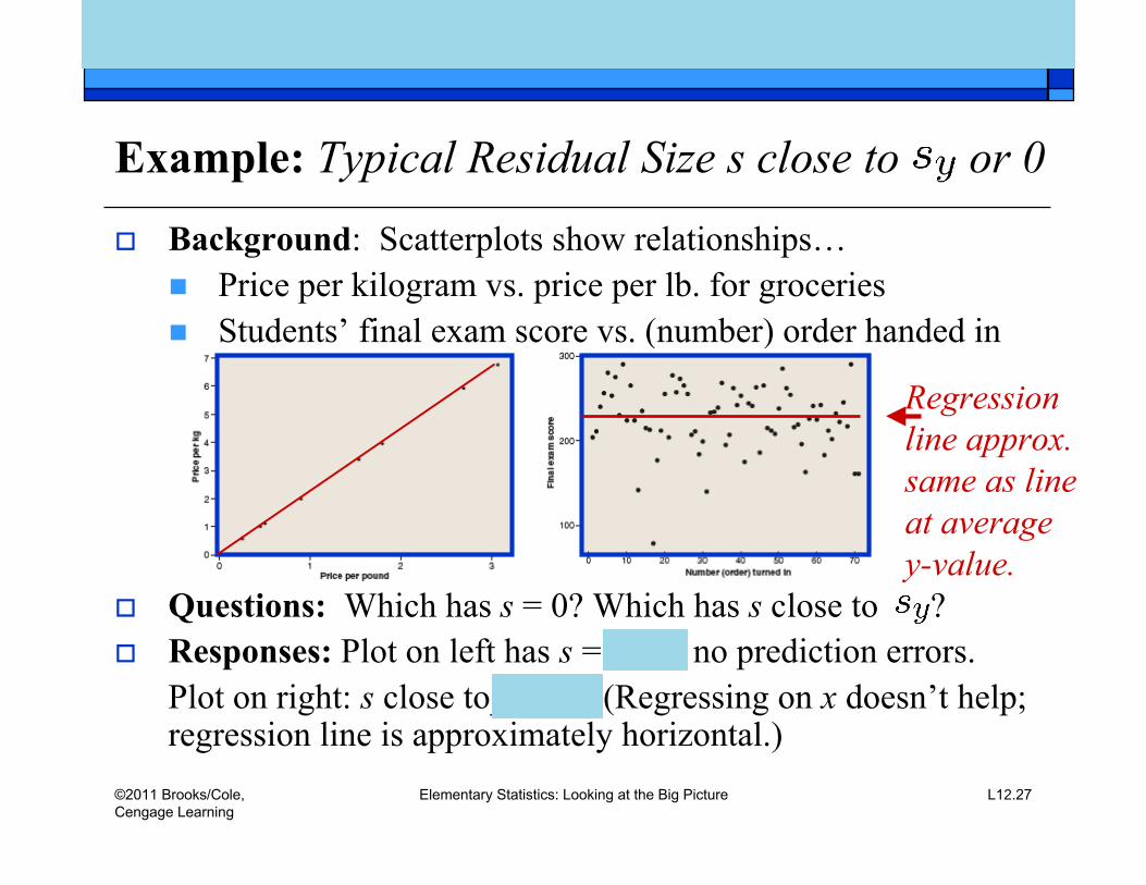
Example: Typical Residual Size s close to or 0

Background: Scatterplots show relationships… Price per kilogram vs. price per lb. for groceries Students’ final exam score vs. (number) order handed in

Questions: Which has s = 0? Which has s close to ? Responses: Plot on left has s =____: no prediction errors.

Plot on right: s close to_____. (Regressing on x doesn’t help;regression line is approximately horizontal.)

Regressionline approx.same as lineat averagey-value.

nancyp

Text Box

Practice: 5.58 p.198



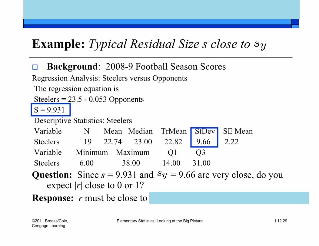
Example: Typical Residual Size s close to

Background: 2008-9 Football Season Scores Regression Analysis: Steelers versus Opponents The regression equation is Steelers = 23.5 - 0.053 Opponents S = 9.931 Descriptive Statistics: Steelers Variable N Mean Median TrMean StDev SE Mean Steelers 19 22.74 23.00 22.82 9.66 2.22 Variable Minimum Maximum Q1 Q3 Steelers 6.00 38.00 14.00 31.00Question: Since s = 9.931 and = 9.66 are very close, do you

expect |r| close to 0 or 1?Response: r must be close to __________________

nancyp

Text Box




Explanatory/Response Roles in RegressionOur choice of roles, explanatory or response,

does not affect the value of the correlation r,but it does affect the regression line.



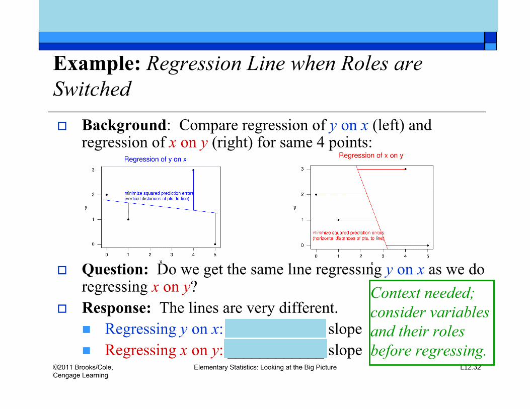
Example: Regression Line when Roles areSwitched Background: Compare regression of y on x (left) and

regression of x on y (right) for same 4 points:

Question: Do we get the same line regressing y on x as we doregressing x on y?

Response: The lines are very different. Regressing y on x: ____________ slope Regressing x on y: ____________ slope

Context needed;consider variablesand their rolesbefore regressing.

nancyp

Text Box

Practice: 5.60b p.198



Definitions Outlier: (in regression) point with unusually

large residual Influential observation: point with high

degree of influence on regression line.



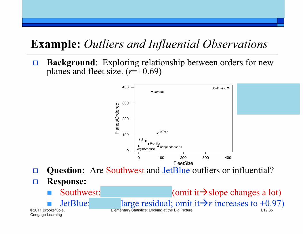
Example: Outliers and Influential Observations Background: Exploring relationship between orders for new

planes and fleet size. (r=+0.69)

Question: Are Southwest and JetBlue outliers or influential? Response:

Southwest: ______________ (omit itslope changes a lot) JetBlue:______(large residual; omit itr increases to +0.97)

nancyp

Text Box

Practice: 5.70d p.203



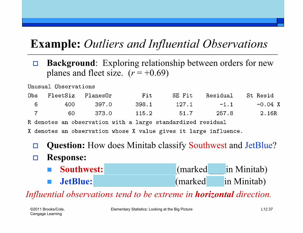
Example: Outliers and Influential Observations Background: Exploring relationship between orders for new

planes and fleet size. (r = +0.69)

Question: How does Minitab classify Southwest and JetBlue? Response:

Southwest: _______________(marked ___ in Minitab) JetBlue: _________________(marked ___ in Minitab)

Influential observations tend to be extreme in horizontal direction.

nancyp

Text Box

Practice: 5.70g p.203



Definitions Slope : how much response y changes in

general (for entire population) for every unitincrease in explanatory variable x

Intercept : where the line that best fits allexplanatory/response points (for entirepopulation) crosses the y-axis

Looking Back: Greek letters often refer topopulation parameters.



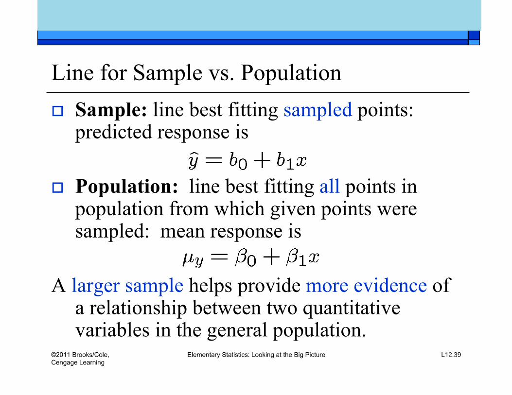
Line for Sample vs. Population Sample: line best fitting sampled points:

predicted response is

Population: line best fitting all points inpopulation from which given points weresampled: mean response is

A larger sample helps provide more evidence ofa relationship between two quantitativevariables in the general population.



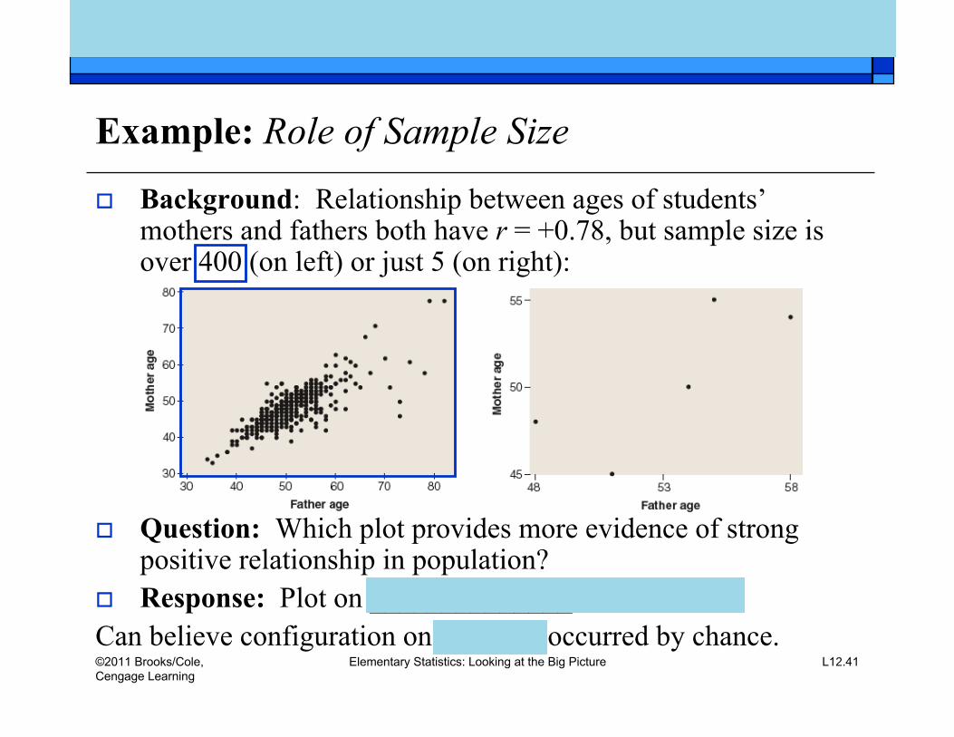
Example: Role of Sample Size

Background: Relationship between ages of students’mothers and fathers both have r = +0.78, but sample size isover 400 (on left) or just 5 (on right):

Question: Which plot provides more evidence of strongpositive relationship in population?

Response: Plot on ______________Can believe configuration on _______ occurred by chance.

nancyp

Text Box




Time SeriesIf explanatory variable is time, plot one response

for each time value and “connect the dots” tolook for general trend over time, also peaksand troughs.



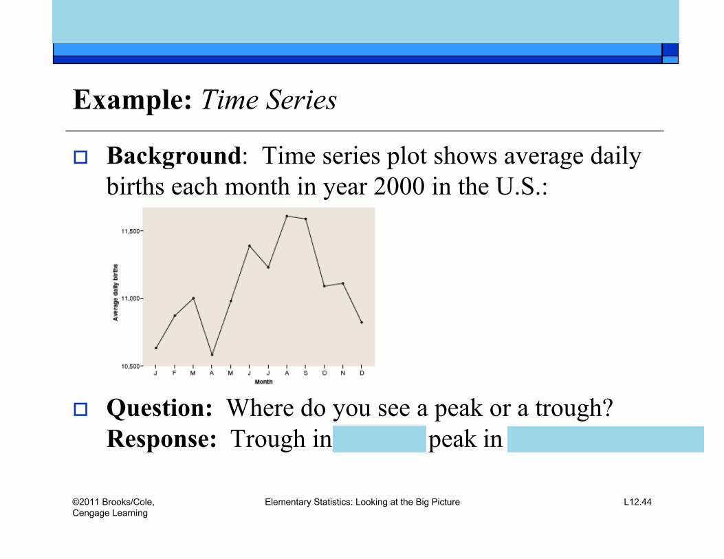
Example: Time Series

Background: Time series plot shows average dailybirths each month in year 2000 in the U.S.:

Question: Where do you see a peak or a trough?Response: Trough in ______, peak in ___________

nancyp

Text Box




Example: Time Series

Background: Time series plot of average daily births in U.S.

Questions: How can we explain why there are… Conceptions in U.S.: fewer in July, more in December? Conceptions in Europe: more in summer, fewer in winter?

Response:A Closer Look: Statistical methods can’t always explain“why”, but at least they help understand “what” is going on.



Additional Variables in Regression Confounding Variable: Combining two

groups that differ with respect to a variablethat is related to both explanatory andresponse variables can affect the nature oftheir relationship.

Multiple Regression: More advancedtreatments consider impact of not just one buttwo or more quantitative explanatoryvariables on a quantitative response.



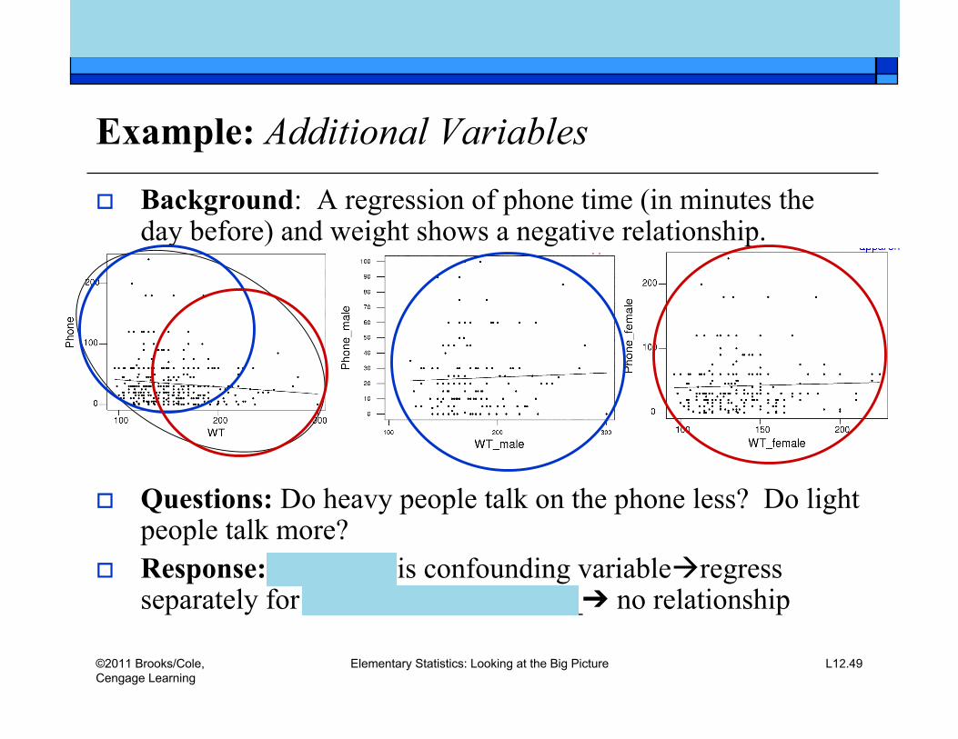
Example: Additional Variables

Background: A regression of phone time (in minutes theday before) and weight shows a negative relationship.

Questions: Do heavy people talk on the phone less? Do lightpeople talk more?

Response: ________ is confounding variableregressseparately for ___________________➔ no relationship

nancyp

Text Box

Practice: 5.113a p.219

nancyp

Oval

nancyp

Oval



Example: Multiple Regression

Background: We used a car’s age to predictits price.

Question: What additional quantitativevariable would help predict a car’s price?

Response:

nancyp

Text Box

Practice: 5.69b-d p.201



Lecture Summary (Regression) Equation of regression line

Interpreting slope and intercept Extrapolation

Residuals: typical size is s Line affected by explanatory/response roles Outliers and influential observations Line for sample or population; role of sample size Time series Additional variables

Lecture 12: more Chapter 5, Section 3 Relationships...

Documents

Transcript of Lecture 12: more Chapter 5, Section 3 Relationships...