Lecture 10 Regulatory motif discovery and target ... · PDF fileLecture 10 Regulatory motif...

Lecture 10 Regulatory motif discovery

and target identification

6.047/6.878 Computational Biology: Genomes, Networks, Evolution

1

Module III: Epigenomics and gene regulation

• Computational Foundations – L10: Gibbs Sampling: between EM and Viterbi training – L11: Rapid linear-time sub-string matching – L11: Multivariate HMMs – L12: Post-transcriptional regulation

• Biological frontiers: – L10: Regulatory motif discovery, TF binding – L11: Epigenomics, chromatin states, differentiation – L12: Post-transcriptional regulation

2

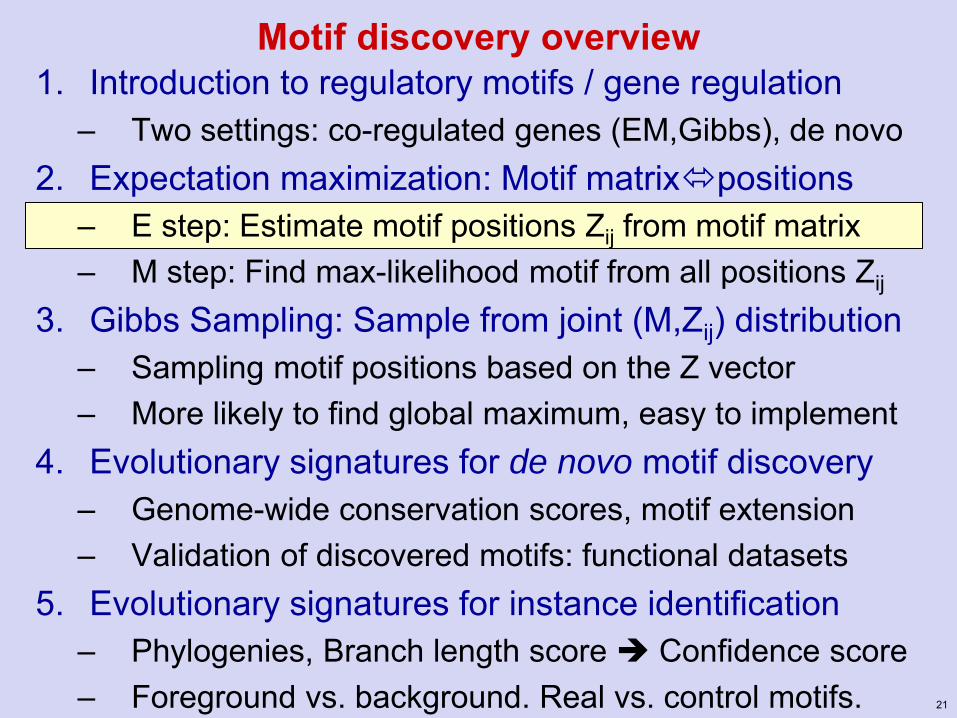
Motif discovery overview 1. Introduction to regulatory motifs / gene regulation

– Two settings: co-regulated genes (EM,Gibbs), de novo 2. Expectation maximization: Motif matrixpositions

– E step: Estimate motif positions Zij from motif matrix – M step: Find max-likelihood motif from all positions Zij

3. Gibbs Sampling: Sample from joint (M,Zij) distribution – Sampling motif positions based on the Z vector – More likely to find global maximum, easy to implement

4. Evolutionary signatures for de novo motif discovery – Genome-wide conservation scores, motif extension – Validation of discovered motifs: functional datasets

5. Evolutionary signatures for instance identification – Phylogenies, Branch length score Confidence score – Foreground vs. background. Real vs. control motifs.

3

ATGACTAAATCTCATTCAGAAGAAGTGA

Regulatory motif discovery

GAL1

CCCCW CGG CCG

Gal4 Mig1

CGG CCG

Gal4

• Regulatory motifs – Genes are turned on / off in response to changing environments – No direct addressing: subroutines (genes) contain sequence tags (motifs) – Specialized proteins (transcription factors) recognize these tags

• What makes motif discovery hard?

– Motifs are short (6-8 bp), sometimes degenerate – Can contain any set of nucleotides (no ATG or other rules) – Act at variable distances upstream (or downstream) of target gene

4

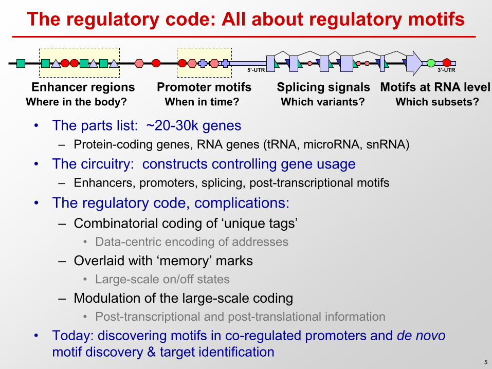
The regulatory code: All about regulatory motifs

• The parts list: ~20-30k genes – Protein-coding genes, RNA genes (tRNA, microRNA, snRNA)

• The circuitry: constructs controlling gene usage – Enhancers, promoters, splicing, post-transcriptional motifs

• The regulatory code, complications: – Combinatorial coding of ‘unique tags’

• Data-centric encoding of addresses – Overlaid with ‘memory’ marks

• Large-scale on/off states – Modulation of the large-scale coding

• Post-transcriptional and post-translational information • Today: discovering motifs in co-regulated promoters and de novo

motif discovery & target identification

Enhancer regions 5’-UTR

Promoter motifs 3’-UTR

Where in the body? When in time? Which variants? Splicing signals

Which subsets? Motifs at RNA level

5

TFs use DNA-binding domains to recognize specific DNA sequences in the genome

DNA-binding domain of Engrailed

“Logo” or “motif”

TAATTA CACGTG AGATAAGA

TCATTA Courtesy of Elsevier, Inc., http://www.sciencedirect.com. Used with permission.Source: Berger, Michael F. et al. "Variation in homeodomain DNA binding revealed byhigh-resolution analysis of sequence preferences." Cell 133, no. 7 (2008): 1266-1276. 6

http://dx.doi.org/10.1016/j.cell.2008.05.024

http://www.sciencedirect.com


Disrupted motif at the heart of FTO obesity locus

Obese

Lean

Strongest association

with obesity

C-to-T disruption of AT-rich

regulatory motif

Restoring motif restores thermogenesis Courtesy of Manolis Kellis. Used with permission. 7

Regulator structure recognized motifs

• Proteins ‘feel’ DNA – Read chemical properties of bases – Do NOT open DNA (no base

complementarity)

• 3D Topology dictates specificity – Fully constrained positions: every atom matters

– “Ambiguous / degenerate” positions loosely contacted

• Other types of recognition

– MicroRNAs: complementarity – Nucleosomes: GC content – RNAs: structure/seqn combination

© Garland Publishing. All rights reserved. This content is excluded from our CreativeCommons license. For more information, see http://ocw.mit.edu/help/faq-fair-use/.

8

http://ocw.mit.edu/help/faq-fair-use/

Motifs summarize TF sequence specificity

• Summarize information

• Integrate many positions

• Measure of information

• Distinguish motif vs. motif instance

• Assumptions: – Independence – Fixed spacing

9

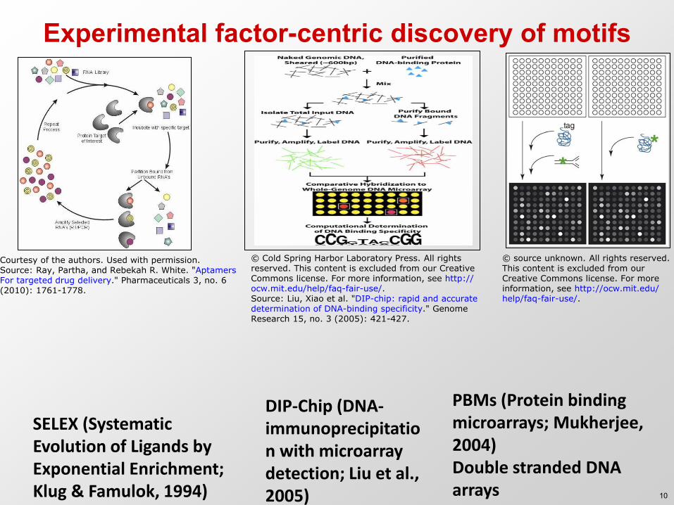
Experimental factor-centric discovery of motifs

SELEX (Systematic Evolution of Ligands by Exponential Enrichment; Klug & Famulok, 1994)

DIP-Chip (DNA-immunoprecipitation with microarray detection; Liu et al., 2005)

PBMs (Protein binding microarrays; Mukherjee, 2004) Double stranded DNA arrays

Courtesy of the authors. Used with permission.Source: Ray, Partha, and Rebekah R. White. "AptamersFor targeted drug delivery." Pharmaceuticals 3, no. 6(2010): 1761-1778.

© Cold Spring Harbor Laboratory Press. All rightsreserved. This content is excluded from our CreativeCommons license. For more information, see http://ocw.mit.edu/help/faq-fair-use/. Source: Liu, Xiao et al. "DIP-chip: rapid and accuratedetermination of DNA-binding specificity." GenomeResearch 15, no. 3 (2005): 421-427.

© source unknown. All rights reserved.This content is excluded from ourCreative Commons license. For moreinformation, see http://ocw.mit.edu/help/faq-fair-use/.

10





http://dx.doi.org/10.1101/gr.3256505

http://dx.doi.org/10.1101/gr.3256505

http://dx.doi.org/10.3390/ph3061761


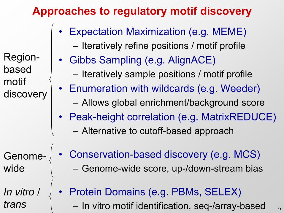
Approaches to regulatory motif discovery

• Expectation Maximization (e.g. MEME) – Iteratively refine positions / motif profile

• Gibbs Sampling (e.g. AlignACE) – Iteratively sample positions / motif profile

• Enumeration with wildcards (e.g. Weeder) – Allows global enrichment/background score

• Peak-height correlation (e.g. MatrixREDUCE) – Alternative to cutoff-based approach

• Conservation-based discovery (e.g. MCS) – Genome-wide score, up-/down-stream bias

• Protein Domains (e.g. PBMs, SELEX) – In vitro motif identification, seq-/array-based

Region-based motif discovery

Genome-wide

In vitro / trans

11

Motifs are not limited to DNA sequences

• Splicing Signals at the RNA level – Splice junctions – Exonic Splicing Enhancers (ESE) – Exonic Splicing Surpressors (ESS)

• Domains and epitopes at the Protein level – Glycosylation sites – Kinase targets – Targetting signals – MHC binding specificities

• Recurring patterns at the physiological level – Expression patterns during the cell cycle – Heart beat patterns predicting cardiac arrest

• Final project in previous year, now used in Boston hospitals! – Any probabilistic recurring pattern

12

Regulator TF/miRNA

Motif Sequence specificity

TFs: Selex, DIP-Chip, Protein-Binding-Microarrays miRNAs: Evolutionary/structural signatures miRNAs: Experimental cloning of 5’-ends

TFs: Mass Spec (difficult)

TFs: ChIP-Chip/ChIP-Seq TFs/miRs: Perturbation response TFs/miRNAs: Evolutionary signatures**

miRNAs: Composition/folding

TFs: Enrichment in co-regulated genes/

bound regions **

TFs: Homology to TFs/domains miRNAs: Evolutionary signatures miRNAs: Experimental cloning

TFs/miRNAs: De novo comparative discovery**

* = Covered in today’s lecture

Network analysis (upcoming lecture)

Challenges in regulatory genomics

Targets Functional instances

Evolutionary footprints DNase footprints Chromatin ‘dips’

13







14

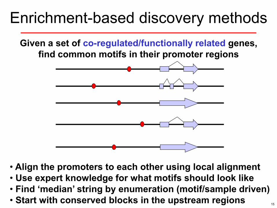
Enrichment-based discovery methods Given a set of co-regulated/functionally related genes,

find common motifs in their promoter regions

• Align the promoters to each other using local alignment • Use expert knowledge for what motifs should look like • Find ‘median’ string by enumeration (motif/sample driven) • Start with conserved blocks in the upstream regions 15

Starting positions Motif matrix

sequence positions

A C G T

1 2 3 4 5 6 7 8

0.1

0.1

0.6

0.2

• given aligned sequences easy to compute profile matrix

0.1

0.5

0.2

0.2 0.3

0.2

0.2

0.3 0.2

0.1

0.5

0.2 0.1

0.1

0.6

0.2

0.3

0.2

0.1

0.4

0.1

0.1

0.7

0.1

0.3

0.2

0.2

0.3

shared motif

given profile matrix • easy to find starting position probabilities

Key idea: Iterative procedure for estimating both, given uncertainty

(learning problem with hidden variables: the starting positions) 16

Basic Iterative Approach

Given: length parameter W, training set of sequences set initial values for motif do re-estimate starting-positions from motif

re-estimate motif from starting-positions until convergence (change < ε)

return: motif, starting-positions

17

Representing Motif M(k,c) and Background B(c)

• Assume motif has fixed width, W • Motif represented by matrix of probabilities: M(k,c)

the probability of character c in column k

1 2 3 A 0.1 0.5 0.2

C 0.4 0.2 0.1

G 0.3 0.1 0.6

T 0.2 0.2 0.1

M

A 0.26

C 0.24

G 0.23

T 0.27

B

• Background represented by B(c), frequency of each base

(near uniform)

(~CAG)

(see also: di-nucleotide etc)

18

Representing the starting position probabilities (Zij)

• the element of the matrix represents the probability that the motif starts in position j in sequence i

Z

1 2 3 4 seq1 0.1 0.1 0.2 0.6

seq2 0.4 0.2 0.1 0.3

seq3 0.3 0.1 0.5 0.1

seq4 0.1 0.5 0.1 0.3

Z

ijZ

Z1

uniform

one big winner

two candidates

no clear winner

Z2

Z3

Z4

Some examples:

19

Starting positions (Zij) Motif matrix M(k,c)

• Zij: Probability that on sequence i, motif start at position j • M(k,c): Probability that kth character of motif is letter c

c=A

c=C

c=G

c=T

k=1 k=2 k=3 k=4 k=5 k=6 k=7 k=8

0.1

0.1

0.6

0.2

0.1

0.5

0.2

0.2 0.3

0.2

0.2

0.3 0.2

0.1

0.5

0.2 0.1

0.1

0.6

0.2

0.3

0.2

0.1

0.4

0.1

0.1

0.7

0.1

0.3

0.2

0.2

0.3

• Three variations for re-computing motif M(k,c) from Zij matrix – Expectation maximization All starts weighted by Zij prob distribution – Gibbs sampling Single start for each seq Xi by sampling Zij

– Greedy approach Best start for each seq Xi by maximum Zij

M-step

E-step

X1 X2 X3 … Xi … Xn Motif: M(k,c) Starting positions: Zij

• Computing Zij matrix from M(k,c) is straightforward – At each position, evaluate start probability by multiplying across the matrix

20







21

E-step: Estimate Zij positions from matrix

c=A

c=C

c=G

c=T

k=1 k=2 k=3 k=4 k=5 k=6 k=7 k=8

0.1

0.1

0.6

0.2

0.1

0.5

0.2

0.2 0.3

0.2

0.2

0.3 0.2

0.1

0.5

0.2 0.1

0.1

0.6

0.2

0.3

0.2

0.1

0.4

0.1

0.1

0.7

0.1

0.3

0.2

0.2

0.3

E-step

X1 X2 X3 … Xi … Xn

Motif: M(k,c) Starting positions: Zij

22

Three examples for Greedy, Gibbs Sampling, EM

uniform

one big winner

two candidates Z1

Z2

Z3

All methods agree

Greedy always picks maximum Gibbs sampling picks one at random (or)

EM uses both in estimating motif (and)

Greedy ignores most of the probability

EM averages over the entire sequence (slow/no convergence)

Gibbs sampling rapidly converges to some choice

23

Calculating P(Xi) when motif position is known

• Probability of training sequence Xi, given hypothesized start position j

L

Wjk

ki

Wj

jk

ki

j

k

kiiji XBXjkMXBBMZX )(),1()(),,1|Pr( ,

1

,

1

1,

before motif motif after motif

A 0.25

C 0.25

G 0.25

T 0.25

MG C T G T A G iX

• Example:

B

0.25 0.251.01.02.00.25 0.25 )()(),3(),2(),1()(B(G)

),,1|Pr( 3

GBABTMGMTMCB

BMZX ii

1 2 3

A 0.1 0.5 0.2

C 0.4 0.2 0.1

G 0.3 0.1 0.6

T 0.2 0.2 0.1

24

Calculating the Z vector ( using M )

• At iteration t, calculate Zij(t) based on M(t)

– We just saw how to calculate Pr(Xi | Zij=1,M(t)) – To obtain total probability Pr(Xi), sum over all starting positions

1

1

)(

)()(

)1Pr(),1|Pr(

)1Pr(),1|Pr(WL

k

ik

t

iki

ij

t

ijit

ij

ZMZX

ZMZXZ

• To estimate the starting positions in Z at step t

(Bayes’ rule)

- Assume uniform priors (motif eq likely to start at any position)

posterior evidence

likelihood prior

)Pr()1Pr(),1|Pr(

),|1Pr()(

)()(

i

ij

t

ijit

iij

t

ijX

ZMZXMXZZ

25

Calculating the Z vector: Example

25.025.025.025.01.02.03.01 iZ

25.025.025.06.02.04.025.02 iZ

• then normalize so that 11

1

WL

j

ijZ...

0 1 2 3

A 0.25 0.1 0.5 0.2

C 0.25 0.4 0.2 0.1

G 0.25 0.3 0.1 0.6

T 0.25 0.2 0.2 0.1

p

G C T G T A G iX

26

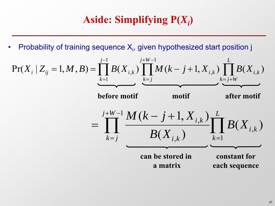
Aside: Simplifying P(Xi)

• Probability of training sequence Xi, given hypothesized start position j

L

k

ki

Wj

jk ki

kiXB

XB

XjkM

1,

1

,

, )()(

),1(

constant for each sequence

can be stored in a matrix

L

Wjk

ki

Wj

jk

ki

j

k

kiiji XBXjkMXBBMZX )(),1()(),,1|Pr( ,

1

,

1

1,

before motif motif after motif

27







28

M-step: Max-likelih motif from Zij positions

c=A

c=C

c=G

c=T

k=1 k=2 k=3 k=4 k=5 k=6 k=7 k=8

0.1

0.1

0.6

0.2

0.1

0.5

0.2

0.2 0.3

0.2

0.2

0.3 0.2

0.1

0.5

0.2 0.1

0.1

0.6

0.2

0.3

0.2

0.1

0.4

0.1

0.1

0.7

0.1

0.3

0.2

0.2

0.3

M-step

X1 X2 X3 … Xi … Xn

Motif: M(k,c) Starting positions: Zij

29

The M-step: Estimating the motif M

c

ck

ckt

dn

dnckM

)(),(

,

,)1(

i cXj

ijkc

kji

Zn}|{

,1,

pseudo-counts

total # of c’s in data set

• recall represents the probability of character c in position k ; stores values for the background

),( ckM

where

)(cB

W

j

cjcc nnn1

,,0

c

c

ct

dn

dncB

)()(

,0

,0)1(where

30

M-step example: Estimating M(k,c) from Zij

A G G C A G

A C A G C A

T C A G T C

4 ... 1

),1(4,33,32,11,1

3,31,23,11,1

ZZZZ

ZZZZAM

Z1 = 0.1 0.7 0.1 0.1

Z2 = 0.4 0.1 0.1 0.4

Z3 = 0.2 0.6 0.1 0.1

X1 =

X2 =

X3 =

• EM: sum over full probability – n1,A= 0.1+0.1+0.4+0.1 = 0.7 – n1,C= 0.7+0.4+0.6 = 1.7 – n1,G= 0.1+0.1+0.1+0.1= 0.4 – n1,T= 0.2 = 0.2 – Total: T=0.7+1.7+0.4+0.2 = 3.0

• Normalize and add pseudo-counts

– M(1,A) = (0.7+1)/(T+4) = 1.7/7=0.24 – M(1,C) = (1.7+1)/(T+4) = 2.7/7=0.39 – M(1,G) = (0.4+1)/(T+4) = 1.4/7=0.2 – M(1,T) = (0.2+1)/(T+4) = 1.2/7=0.17

• M(k,c) =

1 2 3

A 0.24 0.39 0.21

C 0.39 0.21 0.18

G 0.2 0.24 0.44

T 0.17 0.16 0.16

Em approach: Avg’em all Gibbs sampling: Sample one Greedy: Select max 31

The EM Algorithm

• EM converges to a local maximum in the likelihood of the data given the model:

i

i BMX ),|Pr(

• Deterministic iterations max direction of ascent • Usually converges in a small number of iterations • Sensitive to initial starting point (i.e. values in M)

32

P(Seq|Model) Landscape

P(Se

quen

ces|

para

ms1

,par

ams2

)

EM searches for parameters to increase P(seqs|parameters)

Useful to think of P(seqs|parameters)

as a function of parameters

EM starts at an initial set of parameters

And then “climbs uphill” until it reaches a local maximum

Where EM starts can make a big difference

© source unknown. All rights reserved. This content is excludedfrom our Creative Commons license. For more information, seehttp://ocw.mit.edu/help/faq-fair-use/.

33


One solution: Search from Many Different Starts

P(Se

quen

ces|

para

ms1

,par

ams2

)

To minimize the effects of local maxima, you should search multiple times from different starting points

MEME uses this idea

Start at many points

Run for one iteration

Choose starting point that got the “highest” and continue


34








35

Three options for assigning points, and their parallels across K-means, HMMs, Motifs

Update assignments (E step) Estimate hidden labels

Algorithm implementing E step in each of the three settings

Update model parameters (M step) max likelihood

Expression clustering

HMM learning

Motif discovery

The hidden label is: Cluster labels State path π Motif positions

Assign each point to best label

K-means: Assign each point to nearest cluster

Viterbi training: label sequence with best path

Greedy: Find best motif match in each sequence

Average of those points assigned to label

Assign each point to all labels, probabilistically

Fuzzy K-means: Assign to all clusters, weighted by proximity

Baum-Welch training: label sequence w all paths (posterior decoding)

MEME: Use all positions as a motif occurrence weighed by motif match score

Average of all points, weighted by membership

Pick one label at random, based on their relative probability

N/A: Assign to a random cluster, sample by proximity

N/A: Sample a single label for each position, according to posterior prob.

Gibbs sampling: Use one position for the motif, by sampling from the match scores

Average of those points assigned to label(a sample)

Upd

ate

rule

P

ick

a be

st

Aver

age

all

Sam

ple

one

36

Three examples of Greedy, Gibbs Sampling, EM

uniform

one big winner

two candidates Z1

Z2

Z3

All methods agree

Greedy always picks maximum Gibbs sampling picks one at random (or)

EM uses both in estimating motif (and)

Greedy ignores most of the probability

EM averages over the entire sequence (no preference)

Gibbs sampling rapidly converges to some choice

37

Gibbs Sampling • A general procedure for sampling from the joint distribution of a set

of random variables by iteratively sampling from for each j

• Useful when it’s hard to explicitly express means, stdevs, covariances across the multiple dimensions

• Useful for supervised, unsupervised, semi-supervised learning – Specify variables that are known, sample over all other variables

• Approximate: – Joint distribution: the samples drawn – Marginal distributions: examine samples for subset of variables – Expected value: average over samples

• Example of Markov-Chain Monte Carlo (MCMC) – The sample approximates an unknown distribution – Stationary distribution of sample (only start counting after burn-in) – Assume independence of samples (only consider every 100)

• Special case of Metropolis-Hastings – In its basic implementation of sampling step – But it’s a more general sampling framework

) ..., ...|Pr( 111 njjj UUUUU

) ...Pr( 1 nUU

38

Gibbs Sampling for motif discovery

given: length parameter W, training set of sequences choose random positions for a

do pick a sequence Xi

estimate p given current motif positions a (update step) (using all sequences but Xi) sample a new motif position ai for Xi (sampling step) until convergence

return: p, a

• First application to motif finding: Lawrence et al 1993 • Can view as a stochastic analog of EM for motif discovery task • Less susceptible to local minima than EM

• EM maintains distribution Zi over the starting points for each seq • Gibbs sampling selects specific starting point ai for each seq but keeps resampling these starting points

39

Popular implementation: AlignACE, BioProspector AlignACE: first statistical motif finder BioProspector: improved version of AlignACE

Both use basic Gibbs Sampling algorithm: 1. Initialization:

a. Select random locations in sequences X1, …, XN b. Compute an initial model M from these locations

2. Sampling Iterations: a. Remove one sequence Xi b. Recalculate model c. Pick a new location of motif in Xi according to probability

the location is a motif occurrence

In practice, run algorithm from multiple random initializations: 1. Initialize 2. Run until convergence 3. Repeat 1,2 several times, report common motifs

40

Gibbs Sampling (AlignACE) • Given:

– X1, …, XN, – motif length W, – background B,

• Find:

– Model M – Locations a1,…, aN in X1, …, XN

Maximizing log-odds likelihood ratio This is the same as the EM objective (notice log and notation

change)

)(),(

log,

,

1 1 kai

kaiN

i

W

ki

i

XB

XkM

41

Gibbs Sampling (AlignACE) Predictive Update:

• Select a sequence xi • Remove xi, recompute model:

dN

cXdckM is kas s

4)1()(

),( ,

where d is a pseudocount to avoid 0s

M

42

Sampling New Motif Positions

• for each possible starting position, ai=j, compute a weight

• randomly select a new starting position ai according to these weights (normalizing across the sequence, again like with MEME)

• Note, this is equivalent to using the likelihood from MEME because:

),1|Pr( pZXA ijij

1

,

,

)(),1(Wj

jk ki

ki

jXB

XjkMA

0 |x|

Prob

43

Advantages / Disadvantages • Very similar to EM

Advantages: • Easier to implement • Less dependent on initial parameters • More versatile, easier to enhance with heuristics

Disadvantages: • More dependent on all sequences to exhibit the motif • Less systematic search of initial parameter space

44

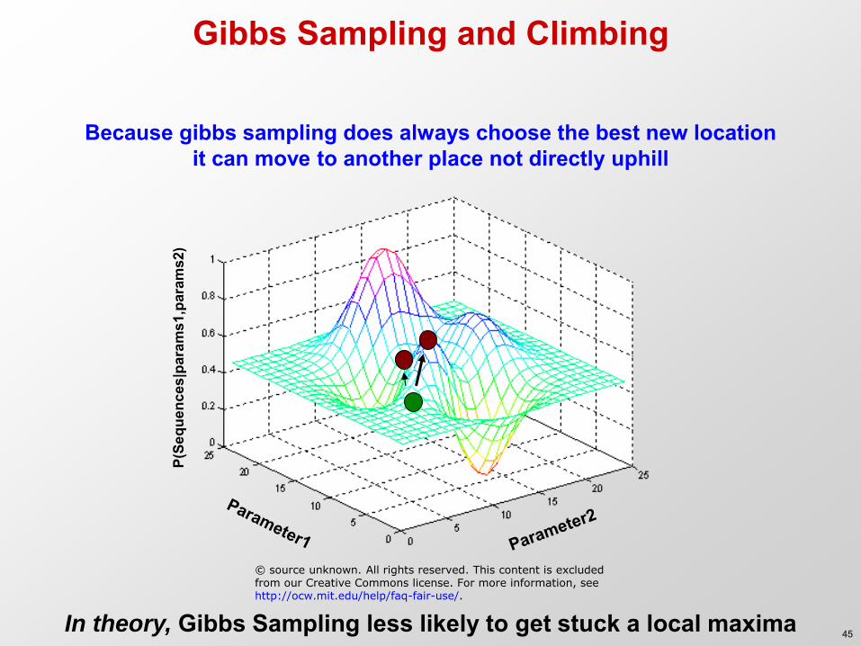
Gibbs Sampling and Climbing

P(Se

quen

ces|

para

ms1

,par

ams2

)

Because gibbs sampling does always choose the best new location it can move to another place not directly uphill

In theory, Gibbs Sampling less likely to get stuck a local maxima


45








46

Motivation for de novo genome-wide motif discovery

• Both TF and region centric approaches are not comprehensive and are biased

• TF centric approaches generally require transcription factor (or antibody to factor) – Lots of time and money – Also have computational challenges

• De novo discovery using conservation is unbiased but can’t match motif to factor and require multiple genomes

47

Evolutionary signatures for regulatory motifs

• Start by looking at known motif instances

• Individual motif instances are preferentially conserved

• Can we just take conservation islands and call them motifs?

– No. Many conservation islands are due to chance or perhaps due to non-motif conservation

Kellis el al, Nature 2003 Xie et al. Nature 2005

Stark et al, Nature 2007

D.mel CAGCT--AGCC-AACTCTCTAATTAGCGACTAAGTC-CAAGTC D.sim CAGCT--AGCC-AACTCTCTAATTAGCGACTAAGTC-CAAGTC D.sec CAGCT--AGCC-AACTCTCTAATTAGCGACTAAGTC-CAAGTC D.yak CAGC--TAGCC-AACTCTCTAATTAGCGACTAAGTC-CAAGTC D.ere CAGCGGTCGCCAAACTCTCTAATTAGCGACCAAGTC-CAAGTC D.ana CACTAGTTCCTAGGCACTCTAATTAGCAAGTTAGTCTCTAGAG ** * * *********** * **** * **

D.mel

Known engrailed binding site

48

Conservation islands overlap known motifs Scer TATCCATATCTAATCTTACTTATATGTTGT-GGAAAT-GTAAAGAGCCCCATTATCTTAGCCTAAAAAAACC--TTCTCTTTGGAACTTTCAGTAATACG Spar TATCCATATCTAGTCTTACTTATATGTTGT-GAGAGT-GTTGATAACCCCAGTATCTTAACCCAAGAAAGCC--TT-TCTATGAAACTTGAACTG-TACG Smik TACCGATGTCTAGTCTTACTTATATGTTAC-GGGAATTGTTGGTAATCCCAGTCTCCCAGATCAAAAAAGGT--CTTTCTATGGAGCTTTG-CTA-TATG Sbay TAGATATTTCTGATCTTTCTTATATATTATAGAGAGATGCCAATAAACGTGCTACCTCGAACAAAAGAAGGGGATTTTCTGTAGGGCTTTCCCTATTTTG ** ** *** **** ******* ** * * * * * * * ** ** * *** * *** * * * Scer CTTAACTGCTCATTGC-----TATATTGAAGTACGGATTAGAAGCCGCCGAGCGGGCGACAGCCCTCCGACGGAAGACTCTCCTCCGTGCGTCCTCGTCT Spar CTAAACTGCTCATTGC-----AATATTGAAGTACGGATCAGAAGCCGCCGAGCGGACGACAGCCCTCCGACGGAATATTCCCCTCCGTGCGTCGCCGTCT Smik TTTAGCTGTTCAAG--------ATATTGAAATACGGATGAGAAGCCGCCGAACGGACGACAATTCCCCGACGGAACATTCTCCTCCGCGCGGCGTCCTCT Sbay TCTTATTGTCCATTACTTCGCAATGTTGAAATACGGATCAGAAGCTGCCGACCGGATGACAGTACTCCGGCGGAAAACTGTCCTCCGTGCGAAGTCGTCT ** ** ** ***** ******* ****** ***** *** **** * *** ***** * * ****** *** * *** Scer TCACCGG-TCGCGTTCCTGAAACGCAGATGTGCCTCGCGCCGCACTGCTCCGAACAATAAAGATTCTACAA-----TACTAGCTTTT--ATGGTTATGAA Spar TCGTCGGGTTGTGTCCCTTAA-CATCGATGTACCTCGCGCCGCCCTGCTCCGAACAATAAGGATTCTACAAGAAA-TACTTGTTTTTTTATGGTTATGAC Smik ACGTTGG-TCGCGTCCCTGAA-CATAGGTACGGCTCGCACCACCGTGGTCCGAACTATAATACTGGCATAAAGAGGTACTAATTTCT--ACGGTGATGCC Sbay GTG-CGGATCACGTCCCTGAT-TACTGAAGCGTCTCGCCCCGCCATACCCCGAACAATGCAAATGCAAGAACAAA-TGCCTGTAGTG--GCAGTTATGGT ** * ** *** * * ***** ** * * ****** ** * * ** * * ** *** Scer GAGGA-AAAATTGGCAGTAA----CCTGGCCCCACAAACCTT-CAAATTAACGAATCAAATTAACAACCATA-GGATGATAATGCGA------TTAG--T Spar AGGAACAAAATAAGCAGCCC----ACTGACCCCATATACCTTTCAAACTATTGAATCAAATTGGCCAGCATA-TGGTAATAGTACAG------TTAG--G Smik CAACGCAAAATAAACAGTCC----CCCGGCCCCACATACCTT-CAAATCGATGCGTAAAACTGGCTAGCATA-GAATTTTGGTAGCAA-AATATTAG--G Sbay GAACGTGAAATGACAATTCCTTGCCCCT-CCCCAATATACTTTGTTCCGTGTACAGCACACTGGATAGAACAATGATGGGGTTGCGGTCAAGCCTACTCG **** * * ***** *** * * * * * * * * ** Scer TTTTTAGCCTTATTTCTGGGGTAATTAATCAGCGAAGCG--ATGATTTTT-GATCTATTAACAGATATATAAATGGAAAAGCTGCATAACCAC-----TT Spar GTTTT--TCTTATTCCTGAGACAATTCATCCGCAAAAAATAATGGTTTTT-GGTCTATTAGCAAACATATAAATGCAAAAGTTGCATAGCCAC-----TT Smik TTCTCA--CCTTTCTCTGTGATAATTCATCACCGAAATG--ATGGTTTA--GGACTATTAGCAAACATATAAATGCAAAAGTCGCAGAGATCA-----AT Sbay TTTTCCGTTTTACTTCTGTAGTGGCTCAT--GCAGAAAGTAATGGTTTTCTGTTCCTTTTGCAAACATATAAATATGAAAGTAAGATCGCCTCAATTGTA * * * *** * ** * * *** *** * * ** ** * ******** **** * Scer TAACTAATACTTTCAACATTTTCAGT--TTGTATTACTT-CTTATTCAAAT----GTCATAAAAGTATCAACA-AAAAATTGTTAATATAC Spar TAAATAC-ATTTGCTCCTCCAAGATT--TTTAATTTCGT-TTTGTTTTATT----GTCATGGAAATATTAACA-ACAAGTAGTTAATATAC Smik TCATTCC-ATTCGAACCTTTGAGACTAATTATATTTAGTACTAGTTTTCTTTGGAGTTATAGAAATACCAAAA-AAAAATAGTCAGTATCT Sbay TAGTTTTTCTTTATTCCGTTTGTACTTCTTAGATTTGTTATTTCCGGTTTTACTTTGTCTCCAATTATCAAAACATCAATAACAAGTATTC * * * * * * ** *** * * * * ** ** ** * * * * * ***

GAL1

TBP

GAL4 GAL4 GAL4

GAL4

MIG1

TBP MIG1

Transcription factor binding Conservation island GAL4

Increase power by testing conservation in many regions

ATGACTA

49

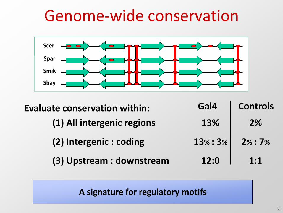
Genome-wide conservation

Evaluate conservation within: Gal4 Controls

13% : 3% 2% : 7% (2) Intergenic : coding

12:0 1:1 (3) Upstream : downstream

A signature for regulatory motifs

13% 2% (1) All intergenic regions

Spar

Smik

Sbay

Scer

50

Test 1: Intergenic conservation

Total count

Co

nse

rve

d c

ou

nt

CGG-11-CCG

© source unknown. All rights reserved. This content is excluded from our CreativeCommons license. For more information, see http://ocw.mit.edu/help/faq-fair-use/.

51


Test 2: Intergenic vs. Coding

Coding Conservation

Inte

rge

nic

Co

nse

rvat

ion

CGG-11-CCG

Higher Conservation in Genes

© source unknown. All rights reserved. This content is excluded from our CreativeCommons license. For more information, see http://ocw.mit.edu/help/faq-fair-use/. 52


Test 3: Upstream vs. Downstream

CGG-11-CCG

Downstream motifs?

Most Patterns

Downstream Conservation

Up

stre

am C

on

serv

atio

n



Conservation for TF motif discovery

1. Enumerate motif seeds

• Six non-degenerate characters with variable size gap in the

middle 2. Score seed motifs

• Use a conservation ratio corrected for composition and small counts to rank seed motifs

3. Expand seed motifs

• Use expanded nucleotide IUPAC alphabet to fill unspecified bases around seed using hill climbing

4. Cluster to remove redundancy • Using sequence similarity

G T C A G T R R Y gap S W

G T C A G T gap

Kellis, Nature 2003 54

Learning motif degeneracy using evolution

• Record frequency with which one sequence is “replaced” by another in evolution

• Use this to find clusters of k-mers that correspond to a single motif

Tanay, Genome Research 2004

© Cold Spring Harbor Laboratory Press. All rights reserved. This content is excluded from our

Creative Commons license. For more information, see http://ocw.mit.edu/help/faq-fair-use/.Source: Tanay, Amos et al. "A global view of the selection forces in the evolution of yeast

cis-regulation." Genome Research 14, no. 5 (2004): 829-834.

55


http://dx.doi.org/10.1101/gr.2064404

http://dx.doi.org/10.1101/gr.2064404







56

Validation of the discovered motifs

• Because genome-wide motif discovery is de novo, we can use functional datasets for validation – Enrichment in co-regulated genes – Overlap with TF binding experiments – Enrichment in genes from the same complex – Positional biases with respect to transcription start – Upstream vs. downstream / inter vs. intra-genic bias – Similarity to known transcription factor motifs

• Each of these metrics can also be used for discovery – In general, split metrics into discovery vs. validation – As long as they are independent ! – Strategies that combine them all lose ability to validate

• Directed experimental validation approaches are then needed

57

Similarity to known motifs

• If discovered motifs are real, we expect them to match motifs in large databases of known motifs

• We find this (significantly higher than with random motifs)

• Why not perfect agreement? – Many known motifs are not

conserved – Known motifs are biased; may have

missed real motifs

MCS Discovered motif Known Factor

46.8 GGGCGGR SP-1 34.7 GCCATnTTg YY1 32.7 CACGTG MYC 31.2 GATTGGY NF-Y 30.8 TGAnTCA AP-1 29.7 GGGAGGRR MAZ 29.5 TGACGTMR CREB 26.0 CGGCCATYK NF-MUE1 25.0 TGACCTTG ERR 22.6 CCGGAARY ELK-1 19.8 SCGGAAGY GABP 17.9 CATTTCCK STAT1

MCS Discovered motif Known Factor

65.6 CTAATTAAA en 57.3 TTKCAATTAA repo 54.9 WATTRATTK ara 54.4 AAATTTATGCK prd 51 GCAATAAA vvl

46.7 DTAATTTRYNR Ubx 45.7 TGATTAAT ap 43.1 YMATTAAAA abd-A 41.2 AAACNNGTT 40 RATTKAATT

39.5 GCACGTGT ftz 38.8 AACASCTG br-Z3

70/174 mammalian motifs

35/145 fly motifs

Stark, Natu

re 2

00

7 X

ie, N

ature

20

05

58

Positional bias of motif matches

• Motifs are involved in initiation of transcription Motif matches biased versus TSS

– 10% of fly motifs – 34% of mammalian motifs

Depletion of TF motifs in coding sequence – 57% of fly motifs

Clustering of motif matches – 19% of fly motifs

59

Motifs have functional enrichments

For both fly (top) and mammals (bottom), motifs are enriched in genes expressed in specific tissues Reveals modules of cooperating motifs

Tissues

Mo

tifs

1. Most motifs avoided in

ubiquitously expressed genes

2. Functional clusters emerge


60


Motif instance identification How do we determine the functional binding sites of regulators?

Kheradpour, Stark, Roy, Kellis, Genome Research 2007

TF1 microRNA1 TF2

61

Experimental target identification: ChIP-chip/seq

Limitations : • Antibody availability • Restricted to specific

stages/tissues • Biological functionality of

most binding sites unknown

• Resolution can be limited (can’t usually identify the precise base pairs)

Ren et al., 2000; Iyer et al., 2001 (ChIP-chip) Robertson et al., 2007 (ChIP-seq) © source unknown. All rights reserved. This content is excluded from our Creative

Commons license. For more information, see http://ocw.mit.edu/help/faq-fair-use/. 62


Computational target identification

• Single genome approaches using motif clustering (e.g. Berman 2002; Schroeder 2004; Philippakis 2006) – Requires set of specific factors that act

together – Miss instances of motifs that may occur alone

• Multi-genome approaches (phylogentic footprinting) (e.g. Moses 2004; Blanchette and Tompa 2002; Etwiller 2005; Lewis 2003) – Tend to either require absolute conservation

or have a strict model of evolution 63

Challenges in target identification

• Simple case – Instance fully conserved in orthologous position near genes

• Motif turn-around/movement – Motif instance is not found in orthologous place due to birth/death or

alignment errors

• Distal/missing matches – Due to sequencing/assembly errors or turnover – Distal instances can be difficult to assign to gene


64

http://dx.doi.org/10.1101/gr.2064404

Computing Branch Length Score (BLS)

CTCF

BLS = 2.23sps (78%) Allows for: 1. Mutations permitted by motif

degeneracy 2. Misalignment/movement of motifs within

window (up to hundreds of nucleotides) 3. Missing motif in dense species tree

mutations

missing short branches

movement



Branch Length Score Confidence

1. Evaluate chance likelihood of a given score • Sequence could also be conserved due to overlap

with un-annotated element (e.g. non-coding RNA) 2. Account for differences in motif composition and

length • For example, short motif more likely to be

conserved by chance

66

Branch Length Score Confidence

1. Use motif-specific shuffled control motifs determine the expected number of instances at each BLS by chance alone or due to non-motif conservation

2. Compute Confidence Score as fraction of instances over noise at a given BLS (=1 – false discovery rate) 67

Producing control motifs When evaluating the conservation,

enrichment, etc, of motifs, it is useful to have a set of “control motifs”

1 Produce 100 shuffles of our original motif

2 Filter motifs, requiring they match the genome with about (+/- 20%) of our original motif

3 Sort potential control motifs based on their similarity to other known motifs

4 Cluster potential control motifs and take at most one from each cluster, in increasing order of similarity to known motifs

Original motif

Genome sequence

Known motifs

68

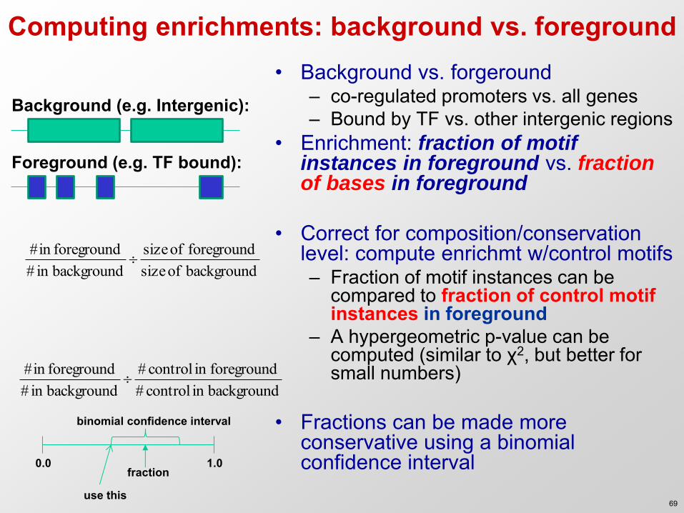
Computing enrichments: background vs. foreground • Background vs. forgeround

– co-regulated promoters vs. all genes – Bound by TF vs. other intergenic regions

• Enrichment: fraction of motif instances in foreground vs. fraction of bases in foreground

• Correct for composition/conservation

level: compute enrichmt w/control motifs – Fraction of motif instances can be

compared to fraction of control motif instances in foreground

– A hypergeometric p-value can be computed (similar to χ2, but better for small numbers)

• Fractions can be made more

conservative using a binomial confidence interval

Foreground (e.g. TF bound):

Background (e.g. Intergenic):

background of sizeforeground of size

backgroundin #foregroundin#

backgroundin control #foregroundin control #

backgroundin #foregroundin#

0.0 1.0 fraction

binomial confidence interval

use this 69

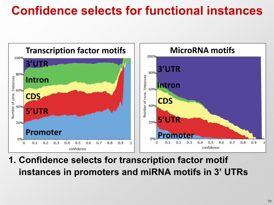
Confidence selects for functional instances

Transcription factor motifs

Promoter

5’UTR

CDS

Intron

3’UTR

MicroRNA motifs

Promoter

5’UTR

CDS

Intron

3’UTR

1. Confidence selects for transcription factor motif instances in promoters and miRNA motifs in 3’ UTRs

70

Validation of discovered motif instances

Use independent experimental evidence Look for functional biases / enrichments

71

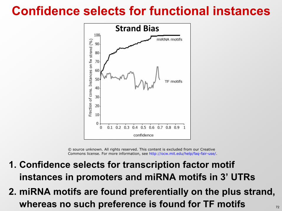
Confidence selects for functional instances

1. Confidence selects for transcription factor motif instances in promoters and miRNA motifs in 3’ UTRs

2. miRNA motifs are found preferentially on the plus strand, whereas no such preference is found for TF motifs

Strand Bias

© source unknown. All rights reserved. This content is excluded from our Creative Commons license. For more information, see http://ocw.mit.edu/help/faq-fair-use/.

72


Increased sensitivity using BLS

73

Figure 3 B removed due to copyright restrictions.Source: Kheradpour, Pouya et al. "Reliable prediction of regulator targets using12 Drosophila genomes." Genome Research 17, no. 12 (2007): 1919-1931.

http://dx.doi.org/10.1101/gr.7090407

http://dx.doi.org/10.1101/gr.7090407

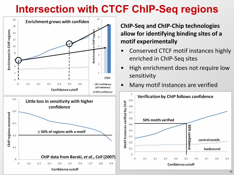
Intersection with CTCF ChIP-Seq regions ChIP-Seq and ChIP-Chip technologies allow for identifying binding sites of a motif experimentally

• Conserved CTCF motif instances highly enriched in ChIP-Seq sites

• High enrichment does not require low sensitivity

• Many motif instances are verified

≥ 50% of regions with a motif

50% motifs verified

50

% co

nfid

ence

ChIP data from Barski, et al., Cell (2007)

74

Enrichment found for many factors

Bar

ski,

et a

l., C

ell (

20

07

)

Od

om

, et

al.

, Na

ture

Gen

etic

s (2

00

7)

Lim

, et

al.

, Mo

lecu

lar

Cel

l (2

00

7)

We

i, et

al.

, Cel

l (2

00

6)

Zelle

r, e

t a

l., P

NA

S (2

00

6)

Lin

, et

al.

, PLo

S G

enet

ics

(20

07

)

Ro

be

rtso

n,

et a

l., N

atu

re M

eth

od

s (2

00

6)

Mammals

Ab

ram

s an

d A

nd

rew

, D

evel

(2

00

5) (

No

t C

hIP

)

San

dm

ann

, et

al.

, Dev

el C

ell (

20

06

)

Zeit

linge

r, e

t a

l., G

enes

& D

evel

(2

00

7)

San

dm

ann

, et

al.

, Gen

es &

Dev

el (

20

07

)

Flies

75

Enrichment increases in conserved bound regions

Human: Barski, et al., Cell (2007) Mouse: Bernstein, unpublished

1. ChIP bound regions may not be conserved 2. For CTCF we also have binding data in mouse 3. Enrichment in intersection is dramatically higher 76

More enrichment when binding conserved

Hu

man

: B

arsk

i, e

t a

l., C

ell (

20

07

) M

ou

se: B

ern

stei

n, u

np

ub

lish

ed

Od

om

, et

al.

, Na

ture

Gen

etic

s (2

00

7)

1. ChIP bound regions may not be conserved 2. For CTCF we also have binding data in mouse 3. Enrichment in intersection is dramatically higher 4. Trend persists for other factors where we have

multi-species ChIP data

77

1. Motifs at 60% confidence and ChIP have similar enrichments (depletion for the repressor Snail) in the functional promoters

2. Enrichments persist even when you look at non-overlapping subsets 3. Intersection of two regions has strongest signal 4. Evolutionary and experimental evidence is complementary

• ChIP includes species specific regions and differentiate tissues • Conserved instances include binding sites not seen in tissues surveyed

ChIP data from: Zeitlinger, et al., G&D (2007); Sandmann, et al,. G&D (2007); Sandmann, et al., Dev Cell (2006)

Comparing ChIP to Conservation

78

TFs: 67 of 83 (81%) 46k instances miRNAs: 49 of 67 (86%) 4k instances

Several connections confirmed by literature (directly or indirectly) Global view of instances allows us to make network level observations: • 46% of targets were co-expressed with their factor in at least one tissue (P < 2 x 10-3) • TFs were more targeted by TFs (P < 10-20) and by miRNAs (P < 5 x 10-5)

• TF in-degree associated with miRNA in-degree (high-high: P < 10-4; low-low P < 10-6)

Fly regulatory network at 60% confidence

© source unknown. All rights reserved. This content is excluded from our Creative Commons license. For more information, see http://ocw.mit.edu/help/faq-fair-use/.

79







80

Regulator TF/miRNA

Motif Sequence specificity

TFs: Selex, DIP-Chip, Protein-Binding-Microarrays miRNAs: Evolutionary/structural signatures miRNAs: Experimental cloning of 5’-ends

TFs: Mass Spec (difficult)

TFs: ChIP-Chip/ChIP-Seq TFs/miRs: Perturbation response TFs/miRNAs: Evolutionary signatures**

miRNAs: Composition/folding

TFs: Enrichment in co-regulated genes/

bound regions **

TFs: Homology to TFs/domains miRNAs: Evolutionary signatures miRNAs: Experimental cloning

TFs/miRNAs: De novo comparative discovery**

* = Covered in today’s lecture

Network analysis (next lecture)

Challenges in regulatory genomics

Targets Functional instances

81

Recitation tomorrow: in vitro motif identification

SELEX (Systematic Evolution of Ligands by Exponential Enrichment; Klug & Famulok, 1994)

PBMs (Protein binding microarrays; Mukherjee, 2004) Double stranded DNA arrays

• PBMs: Protein binding microarrays

• SELEX: Selection-based motif identiifcation

• De Bruijn graphs to generate PBM probes

• From k-mers to motifs • Gapped motifs

• Degenerate motifs and

DNA bending (DNA shape)

• Relaxing independence assumptions in PWMs

Courtesy of the authors. Used with permission. © sSource: Ray, Partha, and Rebekah R. White. This

"Aptamers for targeted drug delivery.“

ource unknown. All rights reserved. content is excluded from our Creative

Commons license. For more information,see http://ocw.mit.edu/help/faq-fair-use/.Pharmaceuticals 3, no. 6 (2010): 1761-1778.

82









83

MIT OpenCourseWarehttp://ocw.mit.edu

6.047 / 6.878 / HST.507 Computational BiologyFall 2015

For information about citing these materials or our Terms of Use, visit: http://ocw.mit.edu/terms.

http://ocw.mit.edu

http://ocw.mit.edu/terms

Lecture 10 Regulatory motif discovery and target ... · PDF fileLecture 10 Regulatory motif...

Documents

Transcript of Lecture 10 Regulatory motif discovery and target ... · PDF fileLecture 10 Regulatory motif...