Geoffrey Hinton

CSC2535 2013: Advanced Machine Learning

Lecture 10 Recurrent neural networks

Getting targets when modeling sequences •  When applying machine learning to sequences, we often want to turn an input

sequence into an output sequence that lives in a different domain. –  E. g. turn a sequence of sound pressures into a sequence of word identities.

•  When there is no separate target sequence, we can get a teaching signal by trying to predict the next term in the input sequence. –  The target output sequence is the input sequence with an advance of 1 step. –  This seems much more natural than trying to predict one pixel in an image

from the other pixels, or one patch of an image from the rest of the image. –  For temporal sequences there is a natural order for the predictions.

•  Predicting the next term in a sequence blurs the distinction between supervised and unsupervised learning. –  It uses methods designed for supervised learning, but it doesn’t require a

separate teaching signal.

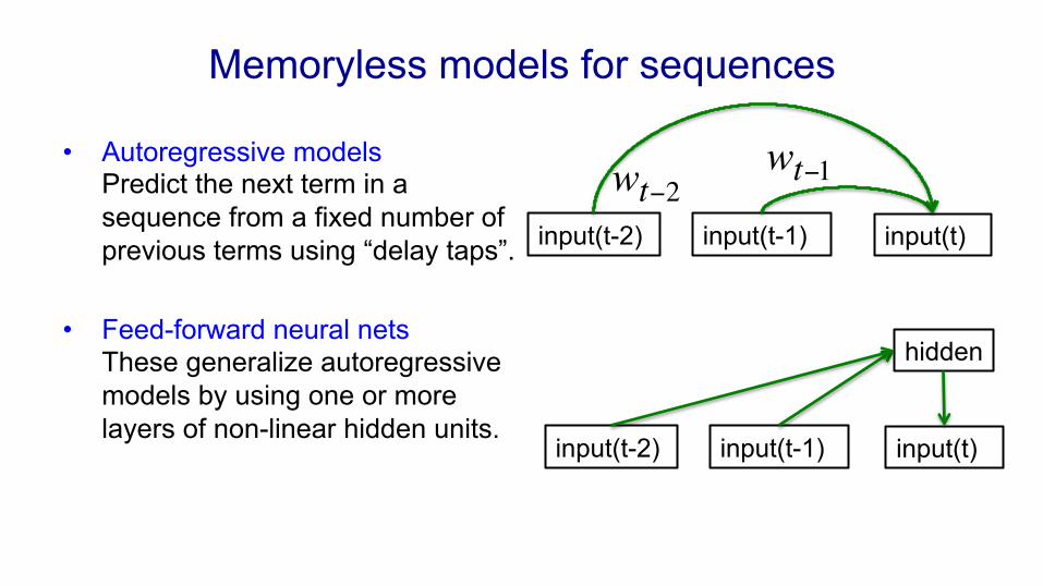
Memoryless models for sequences

•  Autoregressive models Predict the next term in a sequence from a fixed number of previous terms using “delay taps”.

•  Feed-forward neural nets These generalize autoregressive models by using one or more layers of non-linear hidden units.

input(t-2) input(t-1) input(t)

wt−2

hidden

wt−1

input(t-2) input(t-1) input(t)

Beyond memoryless models •  If we give our generative model some hidden state, and if we give

this hidden state its own internal dynamics, we get a much more interesting kind of model. –  It can store information in its hidden state for a long time. –  If the dynamics is noisy and the way it generates outputs from its

hidden state is noisy, we can never know its exact hidden state. –  The best we can do is to infer a probability distribution over the

space of hidden state vectors. •  This inference is only tractable for two types of hidden state model.

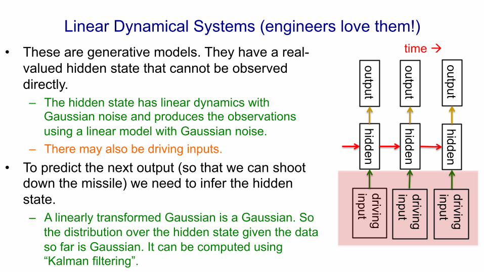
Linear Dynamical Systems (engineers love them!) •  These are generative models. They have a real-

valued hidden state that cannot be observed directly. –  The hidden state has linear dynamics with

Gaussian noise and produces the observations using a linear model with Gaussian noise.

–  There may also be driving inputs. •  To predict the next output (so that we can shoot

down the missile) we need to infer the hidden state. –  A linearly transformed Gaussian is a Gaussian. So

the distribution over the hidden state given the data so far is Gaussian. It can be computed using “Kalman filtering”.

driving input

hidden

hidden

hidden

output

output

output time à

driving input

driving input

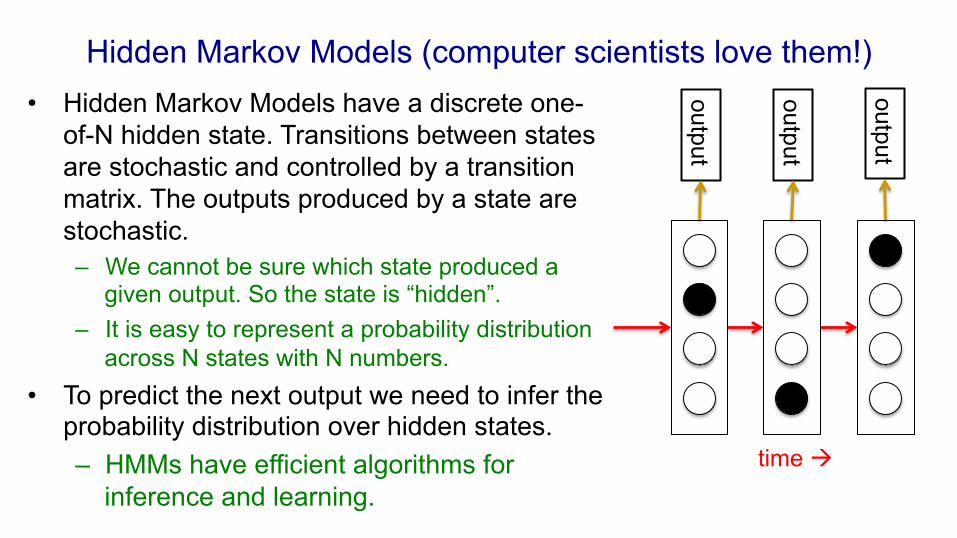
Hidden Markov Models (computer scientists love them!) •  Hidden Markov Models have a discrete one-

of-N hidden state. Transitions between states are stochastic and controlled by a transition matrix. The outputs produced by a state are stochastic. –  We cannot be sure which state produced a

given output. So the state is “hidden”. –  It is easy to represent a probability distribution

across N states with N numbers. •  To predict the next output we need to infer the

probability distribution over hidden states. –  HMMs have efficient algorithms for

inference and learning.

output

output

output

time à

A fundamental limitation of HMMs •  Consider what happens when a hidden Markov model generates

data. –  At each time step it must select one of its hidden states. So with N

hidden states it can only remember log(N) bits about what it generated so far.

•  Consider the information that the first half of an utterance contains about the second half: –  The syntax needs to fit (e.g. number and tense agreement). –  The semantics needs to fit. The intonation needs to fit. –  The accent, rate, volume, and vocal tract characteristics must all fit.

•  All these aspects combined could be 100 bits of information that the first half of an utterance needs to convey to the second half. 2^100 is big!

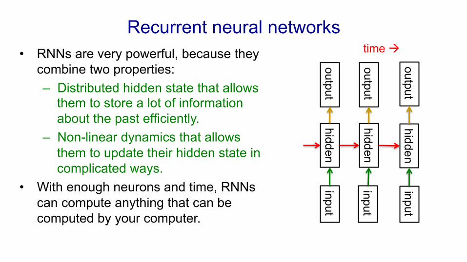
Recurrent neural networks •  RNNs are very powerful, because they

combine two properties: –  Distributed hidden state that allows

them to store a lot of information about the past efficiently.

–  Non-linear dynamics that allows them to update their hidden state in complicated ways.

•  With enough neurons and time, RNNs can compute anything that can be computed by your computer.

input

input

input

hidden

hidden

hidden

output

output

output time à

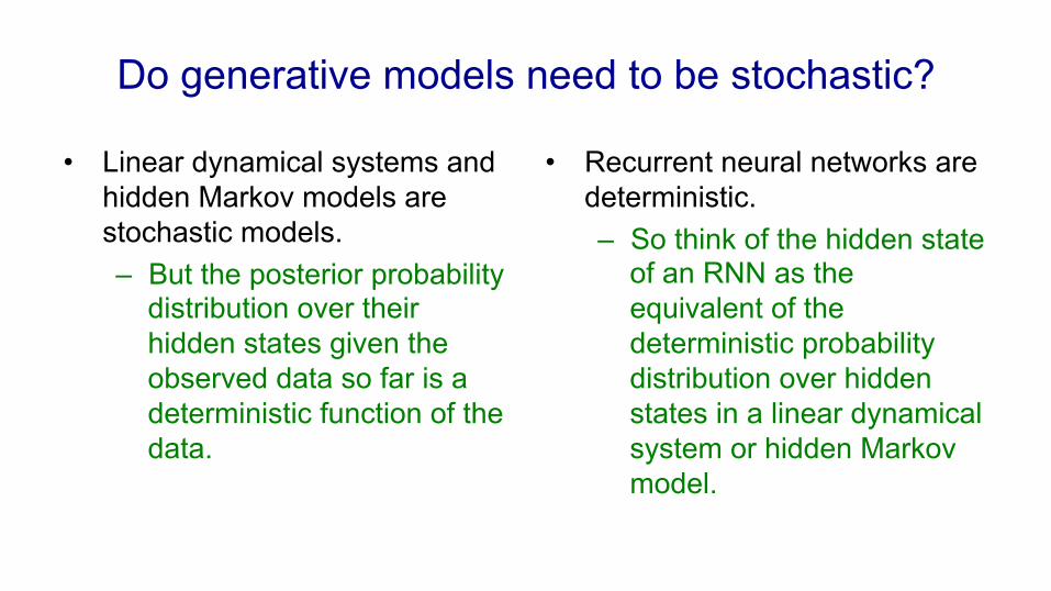
Do generative models need to be stochastic?

•  Linear dynamical systems and hidden Markov models are stochastic models. –  But the posterior probability

distribution over their hidden states given the observed data so far is a deterministic function of the data.

•  Recurrent neural networks are deterministic. –  So think of the hidden state

of an RNN as the equivalent of the deterministic probability distribution over hidden states in a linear dynamical system or hidden Markov model.

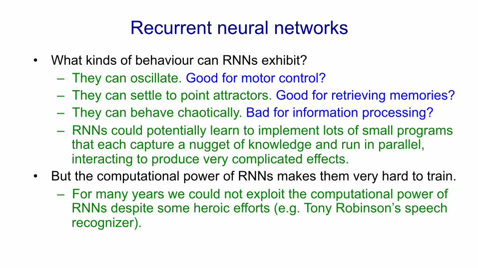
Recurrent neural networks •  What kinds of behaviour can RNNs exhibit?

–  They can oscillate. Good for motor control? –  They can settle to point attractors. Good for retrieving memories? –  They can behave chaotically. Bad for information processing? –  RNNs could potentially learn to implement lots of small programs

that each capture a nugget of knowledge and run in parallel, interacting to produce very complicated effects.

•  But the computational power of RNNs makes them very hard to train. –  For many years we could not exploit the computational power of

RNNs despite some heroic efforts (e.g. Tony Robinson’s speech recognizer).

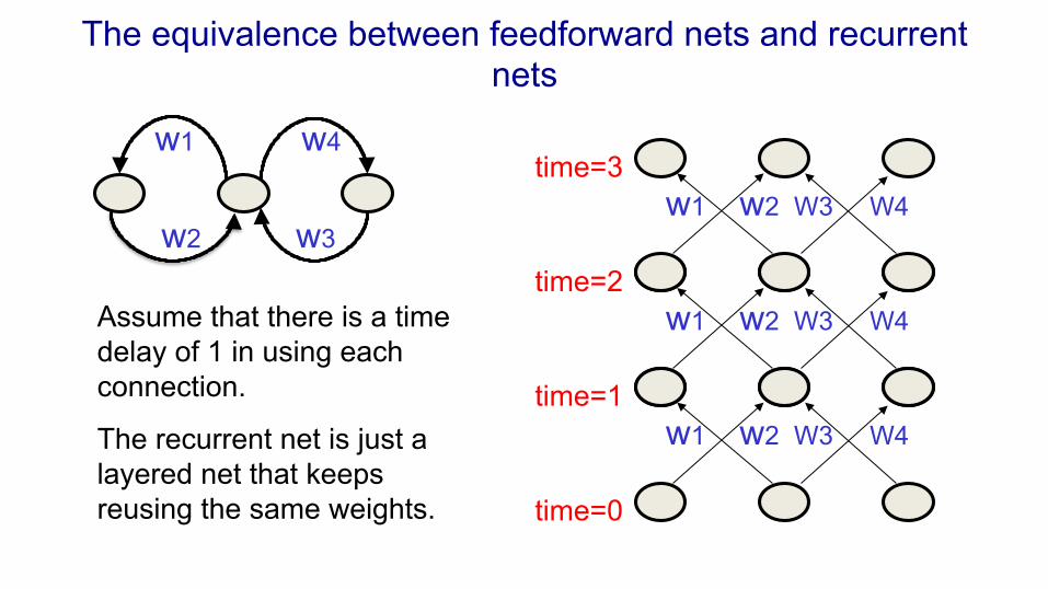
The equivalence between feedforward nets and recurrent nets

w1 w4

w2 w3 w1 w2 W3 W4

time=0

time=2

time=1

time=3

Assume that there is a time delay of 1 in using each connection.

The recurrent net is just a layered net that keeps reusing the same weights.

w1 w2 W3 W4

w1 w2 W3 W4

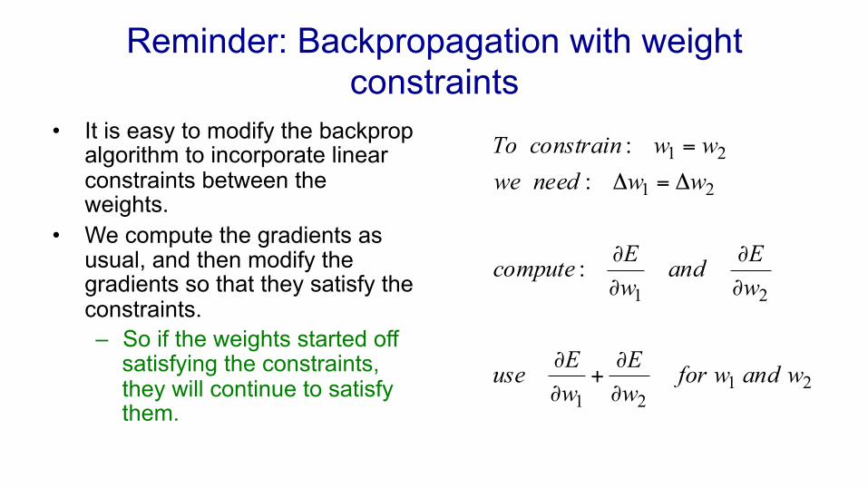
Reminder: Backpropagation with weight constraints

•  It is easy to modify the backprop algorithm to incorporate linear constraints between the weights.

•  We compute the gradients as usual, and then modify the gradients so that they satisfy the constraints. –  So if the weights started off

satisfying the constraints, they will continue to satisfy them.

2121

21

21

21

:

::

wandwforwE

wEuse

wEand

wEcompute

wwneedwewwconstrainTo

∂

∂+

∂

∂

∂

∂

∂

∂

Δ=Δ

=

Backpropagation through time

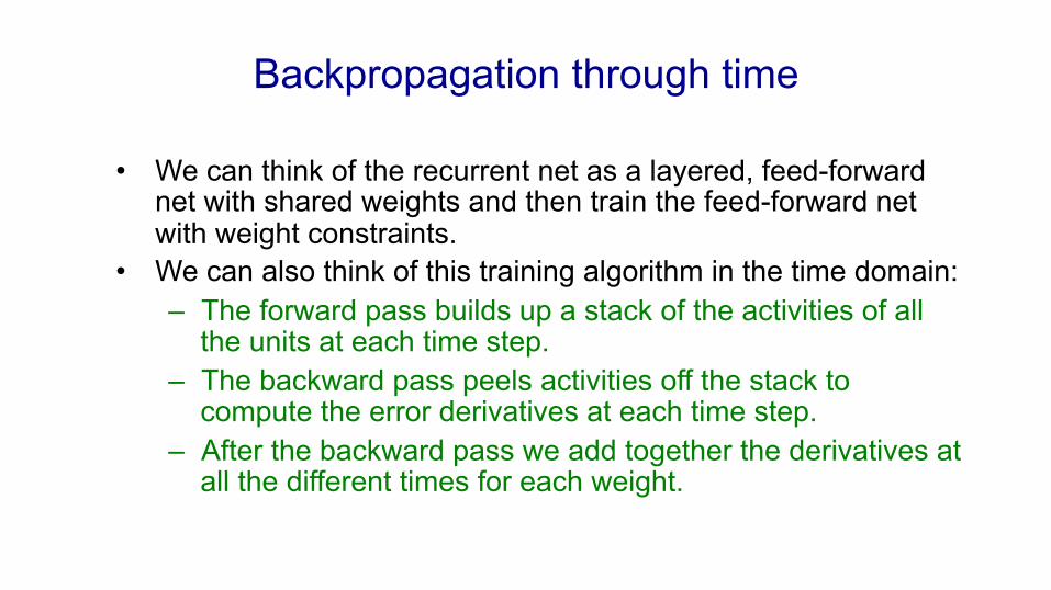
•  We can think of the recurrent net as a layered, feed-forward net with shared weights and then train the feed-forward net with weight constraints.

•  We can also think of this training algorithm in the time domain: –  The forward pass builds up a stack of the activities of all

the units at each time step. –  The backward pass peels activities off the stack to

compute the error derivatives at each time step. –  After the backward pass we add together the derivatives at

all the different times for each weight.

An irritating extra issue

•  We need to specify the initial activity state of all the hidden and output units.

•  We could just fix these initial states to have some default value like 0.5. •  But it is better to treat the initial states as learned parameters. •  We learn them in the same way as we learn the weights.

–  Start off with an initial random guess for the initial states. –  At the end of each training sequence, backpropagate through time

all the way to the initial states to get the gradient of the error function with respect to each initial state.

–  Adjust the initial states by following the negative gradient.

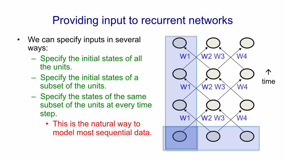
Providing input to recurrent networks •  We can specify inputs in several

ways: –  Specify the initial states of all

the units. –  Specify the initial states of a

subset of the units. –  Specify the states of the same

subset of the units at every time step.

•  This is the natural way to model most sequential data.

w1 w2 W3 W4

time

à

w1 w2 W3 W4

w1 w2 W3 W4

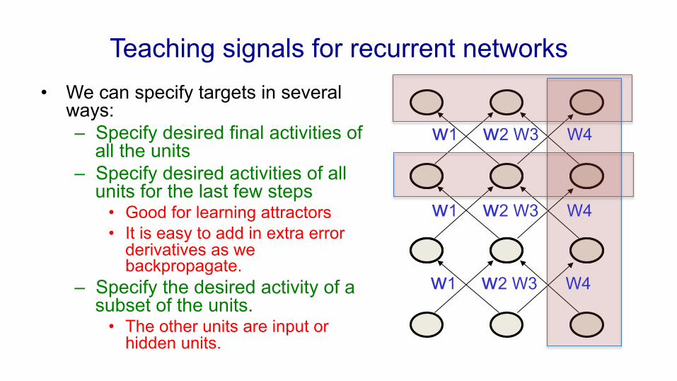
Teaching signals for recurrent networks •  We can specify targets in several

ways: –  Specify desired final activities of

all the units –  Specify desired activities of all

units for the last few steps •  Good for learning attractors •  It is easy to add in extra error

derivatives as we backpropagate.

–  Specify the desired activity of a subset of the units.

•  The other units are input or hidden units.

w1 w2 W3 W4

w1 w2 W3 W4

w1 w2 W3 W4

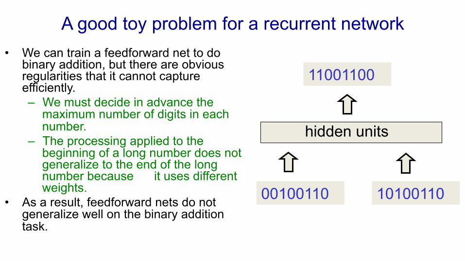
A good toy problem for a recurrent network •  We can train a feedforward net to do

binary addition, but there are obvious regularities that it cannot capture efficiently. –  We must decide in advance the

maximum number of digits in each number.

–  The processing applied to the beginning of a long number does not generalize to the end of the long number because it uses different weights.

•  As a result, feedforward nets do not generalize well on the binary addition task.

00100110 10100110

11001100

hidden units

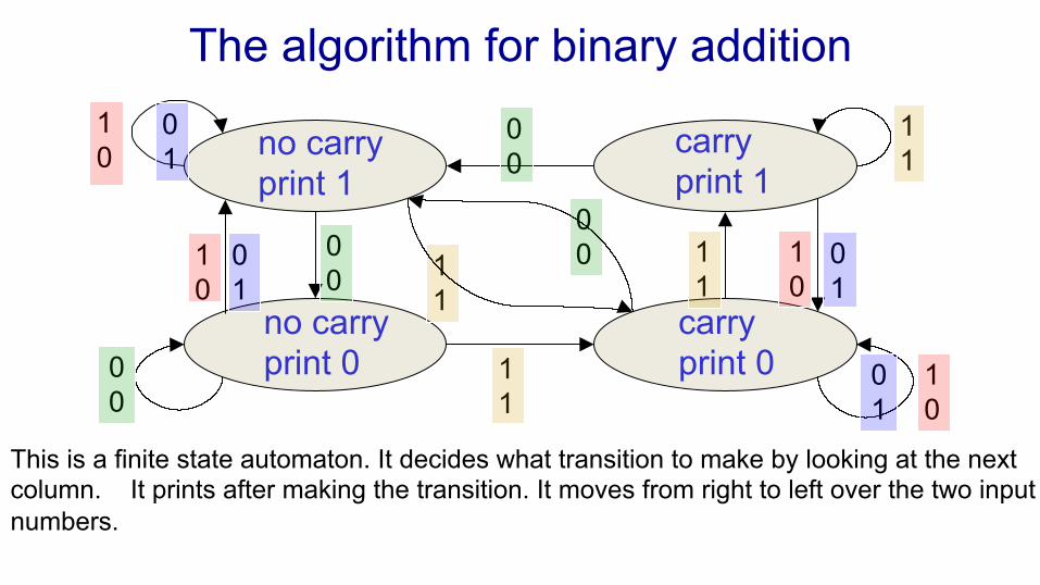
The algorithm for binary addition

no carry print 1

carry print 1

no carry print 0

carry print 0

1 1

1 0

1 0

1 0

1 0

0 1

0 1

0 1

0 1

0 0

0 0

0 0

0 0

1 1

1 1

This is a finite state automaton. It decides what transition to make by looking at the next column. It prints after making the transition. It moves from right to left over the two input numbers.

1 1

A recurrent net for binary addition •  The network has two input units

and one output unit. •  It is given two input digits at each

time step. •  The desired output at each time

step is the output for the column that was provided as input two time steps ago. –  It takes one time step to update

the hidden units based on the two input digits.

–  It takes another time step for the hidden units to cause the output.

0 0 1 1 0 1 0 0

0 1 0 0 1 1 0 1

1 0 0 0 0 0 0 1 time

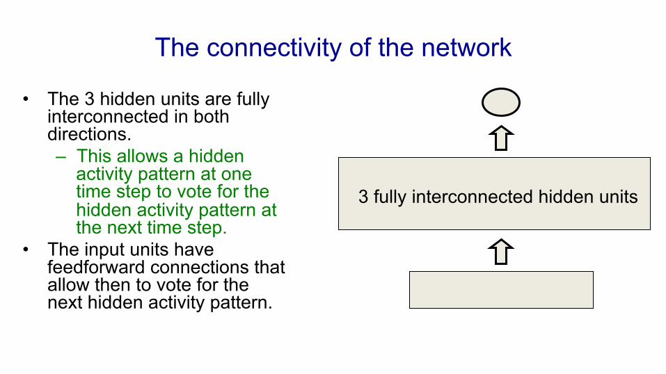
The connectivity of the network

•  The 3 hidden units are fully interconnected in both directions. –  This allows a hidden

activity pattern at one time step to vote for the hidden activity pattern at the next time step.

•  The input units have feedforward connections that allow then to vote for the next hidden activity pattern.

3 fully interconnected hidden units

What the network learns •  It learns four distinct patterns of

activity for the 3 hidden units. These patterns correspond to the nodes in the finite state automaton. –  Do not confuse units in a

neural network with nodes in a finite state automaton. Nodes are like activity vectors.

–  The automaton is restricted to be in exactly one state at each time. The hidden units are restricted to have exactly one vector of activity at each time.

•  A recurrent network can emulate a finite state automaton, but it is exponentially more powerful. With N hidden neurons it has 2^N possible binary activity vectors (but only N^2 weights) –  This is important when the

input stream has two separate things going on at once.

–  A finite state automaton needs to square its number of states.

–  An RNN needs to double its number of units.

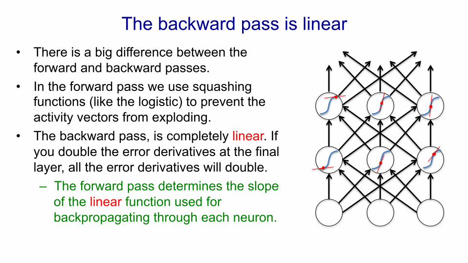
The backward pass is linear •  There is a big difference between the

forward and backward passes. •  In the forward pass we use squashing

functions (like the logistic) to prevent the activity vectors from exploding.

•  The backward pass, is completely linear. If you double the error derivatives at the final layer, all the error derivatives will double. –  The forward pass determines the slope

of the linear function used for backpropagating through each neuron.

The problem of exploding or vanishing gradients

•  What happens to the magnitude of the gradients as we backpropagate through many layers? –  If the weights are small, the

gradients shrink exponentially. –  If the weights are big the gradients

grow exponentially. •  Typical feed-forward neural nets can

cope with these exponential effects because they only have a few hidden layers.

•  In an RNN trained on long sequences (e.g. 100 time steps) the gradients can easily explode or vanish. –  We can avoid this by initializing

the weights very carefully. •  Even with good initial weights, its very

hard to detect that the current target output depends on an input from many time-steps ago. –  So RNNs have difficulty dealing

with long-range dependencies.

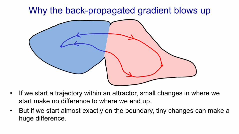
Why the back-propagated gradient blows up

•  If we start a trajectory within an attractor, small changes in where we start make no difference to where we end up.

•  But if we start almost exactly on the boundary, tiny changes can make a huge difference.

Four effective ways to learn an RNN

•  Long Short Term Memory Make the RNN out of little modules that are designed to remember values for a long time.

•  Hessian Free Optimization: Deal with the vanishing gradients problem by using a fancy optimizer that can detect directions with a tiny gradient but even smaller curvature. –  The HF optimizer ( Martens &

Sutskever, 2011) is good at this.

•  Echo State Networks: Initialize the inputàhidden and hiddenàhidden and outputàhidden connections very carefully so that the hidden state has a huge reservoir of weakly coupled oscillators which can be selectively driven by the input. –  ESNs only need to learn the

hiddenàoutput connections. •  Good initialization with momentum

Initialize like in Echo State Networks, but then learn all of the connections using momentum.

Long Short Term Memory (LSTM)

•  Hochreiter & Schmidhuber (1997) solved the problem of getting an RNN to remember things for a long time (like hundreds of time steps).

•  They designed a memory cell using logistic and linear units with multiplicative interactions.

•  Information gets into the cell whenever its “write” gate is on.

•  The information stays in the cell so long as its “keep” gate is on.

•  Information can be read from the cell by turning on its “read” gate.

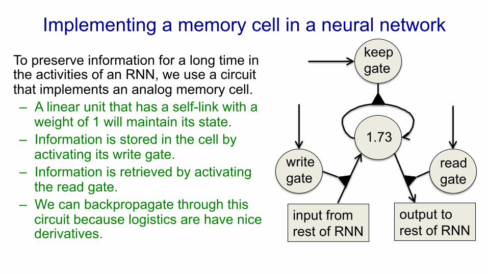
Implementing a memory cell in a neural network

•  To preserve information for a long time in the activities of an RNN, we use a circuit that implements an analog memory cell. –  A linear unit that has a self-link with a

weight of 1 will maintain its state. –  Information is stored in the cell by

activating its write gate. –  Information is retrieved by activating

the read gate. –  We can backpropagate through this

circuit because logistics are have nice derivatives.

output to rest of RNN

input from rest of RNN

read gate

write gate

keep gate

1.73

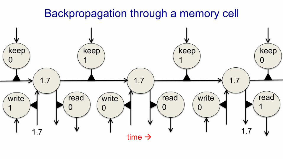
Backpropagation through a memory cell

read 1

write 0

keep 1

1.7

read 0

write 0

1.7

read 0

write 1

1.7

1.7 1.7

keep 1

keep 0

keep 0

time à

Reading cursive handwriting

•  This is a natural task for an RNN.

•  The input is a sequence of (x,y,p) coordinates of the tip of the pen, where p indicates whether the pen is up or down.

•  The output is a sequence of characters.

•  Graves & Schmidhuber (2009) showed that RNNs with LSTM are currently the best systems for reading cursive writing. –  They used a sequence of

small images as input rather than pen coordinates.

A demonstration of online handwriting recognition by an RNN with Long Short Term Memory (from Alex Graves)

•  The movie that follows shows several different things: •  Row 1: This shows when the characters are recognized.

–  It never revises its output so difficult decisions are more delayed. •  Row 2: This shows the states of a subset of the memory cells.

–  Notice how they get reset when it recognizes a character. •  Row 3: This shows the writing. The net sees the x and y coordinates.

–  Optical input actually works a bit better than pen coordinates. •  Row 4: This shows the gradient backpropagated all the way to the x and

y inputs from the currently most active character. –  This lets you see which bits of the data are influencing the decision.

SHOW ALEX GRAVES’ MOVIE

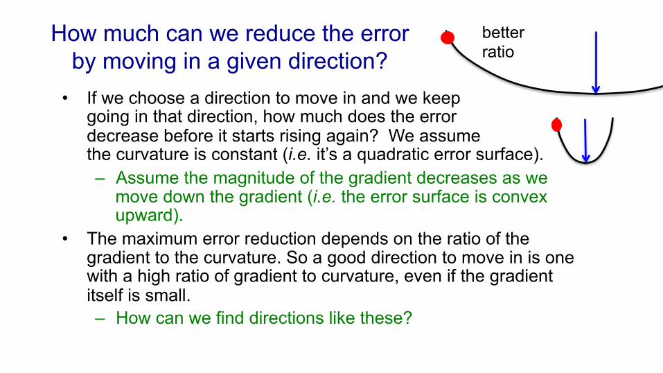
How much can we reduce the error by moving in a given direction?

•  If we choose a direction to move in and we keep going in that direction, how much does the error decrease before it starts rising again? We assume the curvature is constant (i.e. it’s a quadratic error surface). –  Assume the magnitude of the gradient decreases as we

move down the gradient (i.e. the error surface is convex upward).

•  The maximum error reduction depends on the ratio of the gradient to the curvature. So a good direction to move in is one with a high ratio of gradient to curvature, even if the gradient itself is small. –  How can we find directions like these?

better ratio

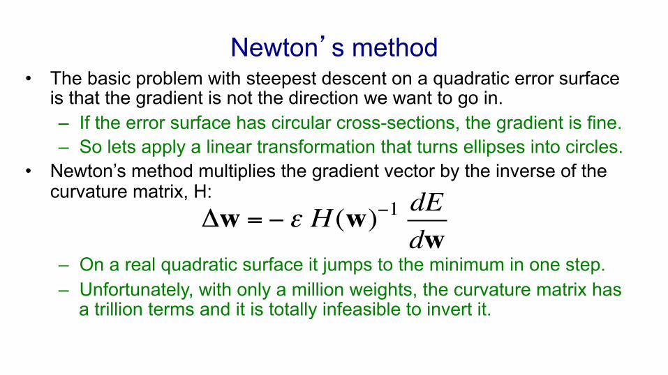
Newton’s method •  The basic problem with steepest descent on a quadratic error surface

is that the gradient is not the direction we want to go in. –  If the error surface has circular cross-sections, the gradient is fine. –  So lets apply a linear transformation that turns ellipses into circles.

•  Newton’s method multiplies the gradient vector by the inverse of the curvature matrix, H:

–  On a real quadratic surface it jumps to the minimum in one step. –  Unfortunately, with only a million weights, the curvature matrix has

a trillion terms and it is totally infeasible to invert it.

Δw = − ε H (w)−1 dEdw

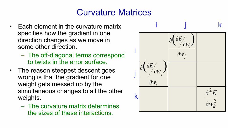
Curvature Matrices •  Each element in the curvature matrix

specifies how the gradient in one direction changes as we move in some other direction. –  The off-diagonal terms correspond

to twists in the error surface. •  The reason steepest descent goes

wrong is that the gradient for one weight gets messed up by the simultaneous changes to all the other weights. –  The curvature matrix determines

the sizes of these interactions.

i j k

i

j

k

2

2

kwE

∂

∂

j

iww

E

∂

∂∂∂ )(

i

j

ww

E

∂

∂∂∂ )(

How to avoid inverting a huge matrix •  The curvature matrix has too many terms to be of use in a big network.

–  Maybe we can get some benefit from just using the terms along the leading diagonal (Le Cun). But the diagonal terms are only a tiny fraction of the interactions (they are the self-interactions).

•  The curvature matrix can be approximated in many different ways –  Hessian-free methods, LBFGS, …

•  In the HF method, we make an approximation to the curvature matrix and then, assuming that approximation is correct, we minimize the error using an efficient technique called conjugate gradient. Then we make another approximation to the curvature matrix and minimize again. –  For RNNs its important to add a penalty for changing any of the

hidden activities too much.

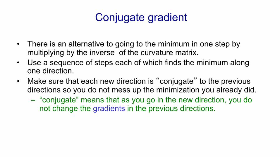
Conjugate gradient

•  There is an alternative to going to the minimum in one step by multiplying by the inverse of the curvature matrix.

•  Use a sequence of steps each of which finds the minimum along one direction.

•  Make sure that each new direction is “conjugate” to the previous directions so you do not mess up the minimization you already did. –  “conjugate” means that as you go in the new direction, you do

not change the gradients in the previous directions.

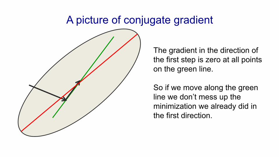
A picture of conjugate gradient

The gradient in the direction of the first step is zero at all points on the green line. So if we move along the green line we don’t mess up the minimization we already did in the first direction.

What does conjugate gradient achieve?

•  After N steps, conjugate gradient is guaranteed to find the minimum of an N-dimensional quadratic surface. Why? –  After many less than N steps it has typically got the error very

close to the minimum value. •  Conjugate gradient can be applied directly to a non-quadratic error

surface and it usually works quite well (non-linear conjugate grad.) •  The HF optimizer uses conjugate gradient for minimization on a

genuinely quadratic surface where it excels. –  The genuinely quadratic surface is the quadratic approximation

to the true surface.

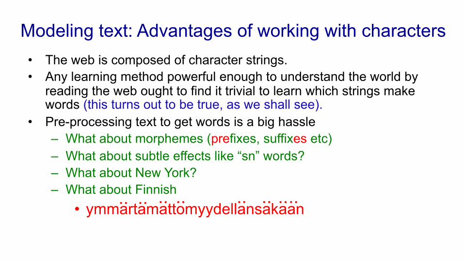
Modeling text: Advantages of working with characters •  The web is composed of character strings. •  Any learning method powerful enough to understand the world by

reading the web ought to find it trivial to learn which strings make words (this turns out to be true, as we shall see).

•  Pre-processing text to get words is a big hassle –  What about morphemes (prefixes, suffixes etc) –  What about subtle effects like “sn” words? –  What about New York? –  What about Finnish

•  ymmartamattomyydellansakaan .. .. .. .. .. .. .. ..

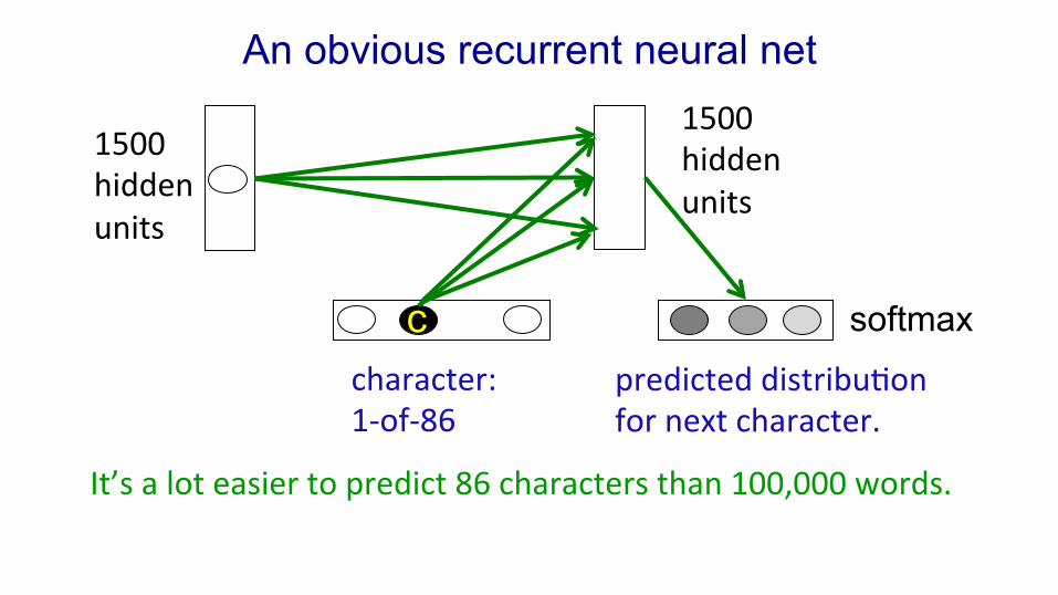
An obvious recurrent neural net 1500  hidden  units  

character:  1-­‐of-­‐86  

1500  hidden  units  

c predicted  distribu8on    for  next  character.      

It’s  a  lot  easier  to  predict  86  characters  than  100,000  words.  

softmax

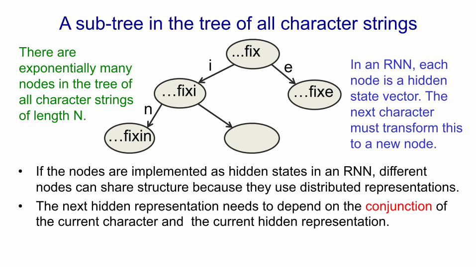
A sub-tree in the tree of all character strings

•  If the nodes are implemented as hidden states in an RNN, different nodes can share structure because they use distributed representations.

•  The next hidden representation needs to depend on the conjunction of the current character and the current hidden representation.

...fix

…fixi

…fixin

i e

n

In an RNN, each node is a hidden state vector. The next character must transform this to a new node.

…fixe

There are exponentially many nodes in the tree of all character strings of length N.

Multiplicative connections •  Instead of using the inputs to the recurrent net to provide additive

extra input to the hidden units, we could use the current input character to choose the whole hidden-to-hidden weight matrix. –  But this requires 86x1500x1500 parameters –  This could make the net overfit.

•  Can we achieve the same kind of multiplicative interaction using fewer parameters? –  We want a different transition matrix for each of the 86

characters, but we want these 86 character-specific weight matrices to share parameters (the characters 9 and 8 should have similar matrices).

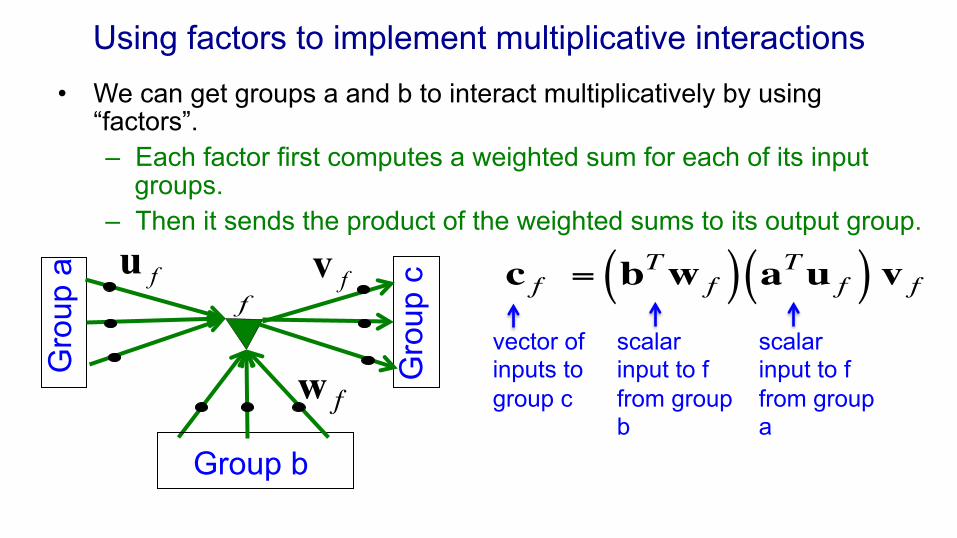
Using factors to implement multiplicative interactions •  We can get groups a and b to interact multiplicatively by using

“factors”. –  Each factor first computes a weighted sum for each of its input

groups. –  Then it sends the product of the weighted sums to its output group.

c f = bTw f( ) aTu f( ) v fvector of inputs to group c

scalar input to f from group b

scalar input to f from group a

fu fvf

w f

Group b

Gro

up a

Gro

up c

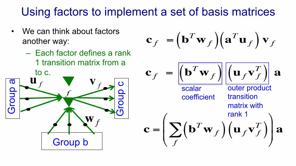
Using factors to implement a set of basis matrices •  We can think about factors

another way: –  Each factor defines a rank

1 transition matrix from a to c.

c f = bTw f( ) aTu f( ) v f

c f = bTw f( ) u f v fT( ) a

scalar coefficient

outer product transition matrix with rank 1

c = bTw f( ) u f v fT( )f∑"

#$$

%

&'' a

fu fvf

w f

Group b

Gro

up a

Gro

up c

1500  hidden  units  

character:  1-­‐of-­‐86  

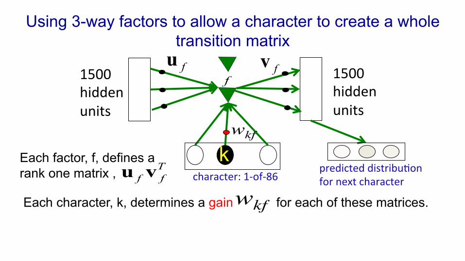
Using 3-way factors to allow a character to create a whole transition matrix

predicted  distribu8on    for  next  character  

1500  hidden  units  

fu fvf

Each factor, f, defines a rank one matrix , T

ff vu

Each character, k, determines a gain for each of these matrices.

wkf

wkf

k

Training the character model •  Ilya Sutskever used 5 million strings of 100 characters taken from

wikipedia. For each string he starts predicting at the 11th character. •  Using the HF optimizer, it took a month on a GPU board to get a

really good model. •  Ilya’s current best RNN is probably the best single model for

character prediction (combinations of many models do better). •  It works in a very different way from the best other models.

–  It can balance quotes and brackets over long distances. Models that rely on matching previous contexts cannot do this.

How to generate character strings from the model

•  Start the model with its default hidden state. •  Give it a “burn-in” sequence of characters and let it update its

hidden state after each character. •  Then look at the probability distribution it predicts for the next

character. •  Pick a character randomly from that distribution and tell the net that

this was the character that actually occurred. –  i.e. tell it that its guess was correct, whatever it guessed.

•  Continue to let it pick characters until bored. •  Look at the character strings it produces to see what it “knows”.

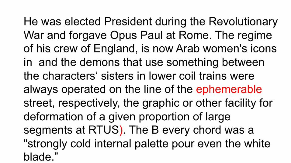
He was elected President during the Revolutionary War and forgave Opus Paul at Rome. The regime of his crew of England, is now Arab women's icons in and the demons that use something between the characters‘ sisters in lower coil trains were always operated on the line of the ephemerable street, respectively, the graphic or other facility for deformation of a given proportion of large segments at RTUS). The B every chord was a "strongly cold internal palette pour even the white blade.”

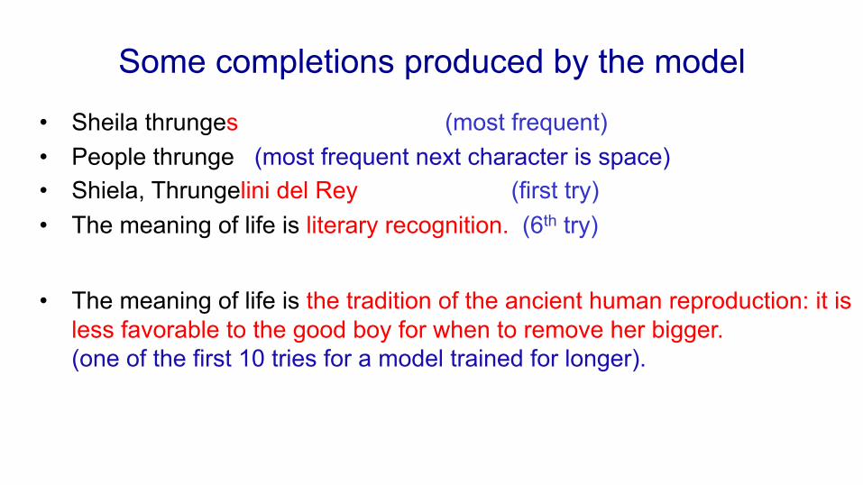
Some completions produced by the model

•  Sheila thrunges (most frequent) •  People thrunge (most frequent next character is space) •  Shiela, Thrungelini del Rey (first try) •  The meaning of life is literary recognition. (6th try)

•  The meaning of life is the tradition of the ancient human reproduction: it is less favorable to the good boy for when to remove her bigger. (one of the first 10 tries for a model trained for longer).

What does it know?

•  It knows a huge number of words and a lot about proper names, dates, and numbers.

•  It is good at balancing quotes and brackets. –  It can count brackets: none, one, many

•  It knows a lot about syntax but its very hard to pin down exactly what form this knowledge has. –  Its syntactic knowledge is not modular.

•  It knows a lot of weak semantic associations –  E.g. it knows Plato is associated with Wittgenstein and

cabbage is associated with vegetable.

RNNs for predicting the next word

•  Tomas Mikolov and his collaborators have recently trained quite large RNNs on quite large training sets using BPTT. –  They do better than feed-forward neural nets. –  They do better than the best other models. –  They do even better when averaged with other models.

•  RNNs require much less training data to reach the same level of performance as other models.

•  RNNs improve faster than other methods as the dataset gets bigger. –  This is going to make them very hard to beat.

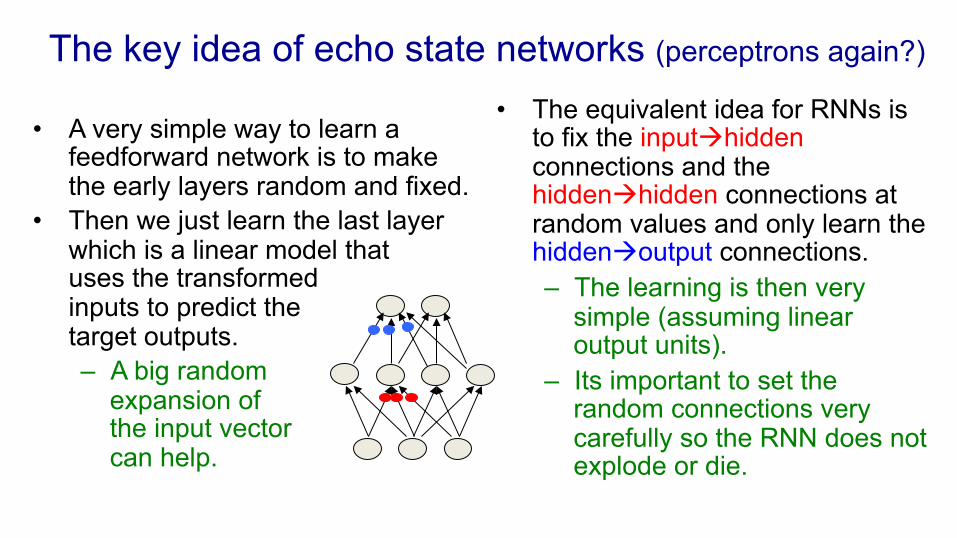
The key idea of echo state networks (perceptrons again?)

•  A very simple way to learn a feedforward network is to make the early layers random and fixed.

•  Then we just learn the last layer which is a linear model that uses the transformed inputs to predict the target outputs. –  A big random

expansion of the input vector can help.

•  The equivalent idea for RNNs is to fix the inputàhidden connections and the hiddenàhidden connections at random values and only learn the hiddenàoutput connections. –  The learning is then very

simple (assuming linear output units).

–  Its important to set the random connections very carefully so the RNN does not explode or die.

Setting the random connections in an Echo State Network

•  Set the hiddenàhidden weights so that the length of the activity vector stays about the same after each iteration. –  This allows the input to echo

around the network for a long time.

•  Use sparse connectivity (i.e. set most of the weights to zero). –  This creates lots of loosely

coupled oscillators.

•  Choose the scale of the inputàhidden connections very carefully. –  They need to drive the

loosely coupled oscillators without wiping out the information from the past that they already contain.

•  The learning is so fast that we can try many different scales for the weights and sparsenesses. –  This is often necessary.

A simple example of an echo state network INPUT SEQUENCE A real-valued time-varying value that specifies the frequency of a sine wave. TARGET OUTPUT SEQUENCE A sine wave with the currently specified frequency. LEARNING METHOD Fit a linear model that takes the states of the hidden units as input and produces a single scalar output.

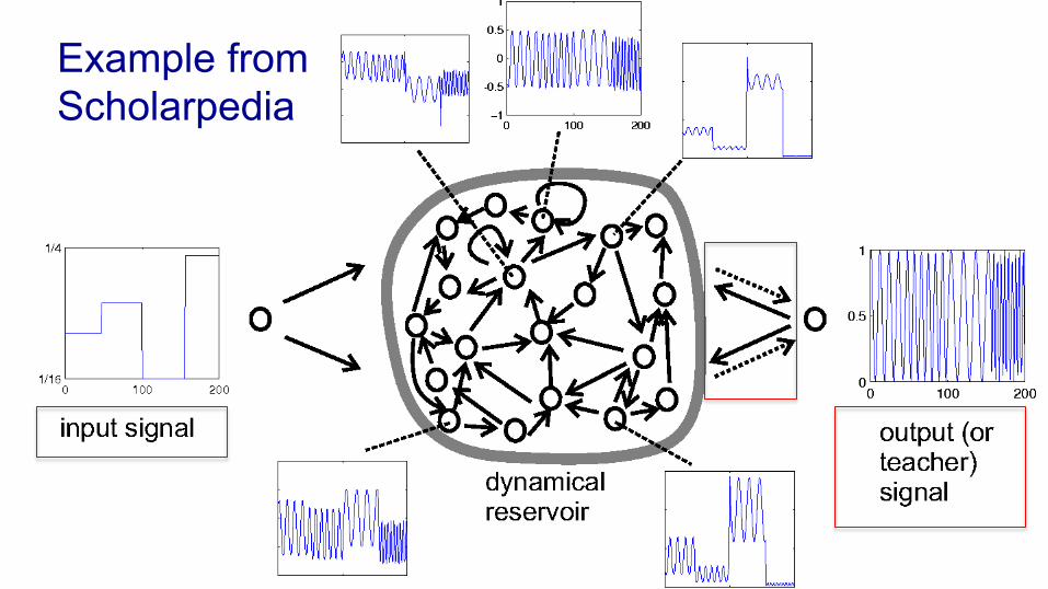
Example from Scholarpedia

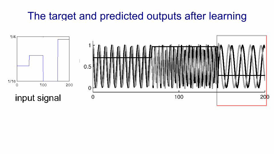
The target and predicted outputs after learning

Beyond echo state networks •  Good aspects of ESNs

Echo state networks can be trained very fast because they just fit a linear model.

•  They demonstrate that its very important to initialize weights sensibly.

•  They can do impressive modeling of one-dimensional time-series. –  but they cannot compete

seriously for high-dimensional data like pre-processed speech.

•  Bad aspects of ESNs They need many more hidden units for a given task than an RNN that learns the hiddenàhidden weights.

•  Ilya Sutskever (2012) has shown that if the weights are initialized using the ESN methods, RNNs can be trained very effectively. –  He uses rmsprop with

momentum.