1

Lecture 1Hardy-Weinberg equilibrium and

key forces affecting gene frequency

Bruce Walsh lecture notesIntroduction to Quantitative Genetics

SISG (Module 9), Seattle15 – 17 July 2019

Outline

• Genetics of complex traits• Stability of distributions over time• Hardy-Weinberg• Multilocus Hardy-Weinberg• Population Structure• Selection

2

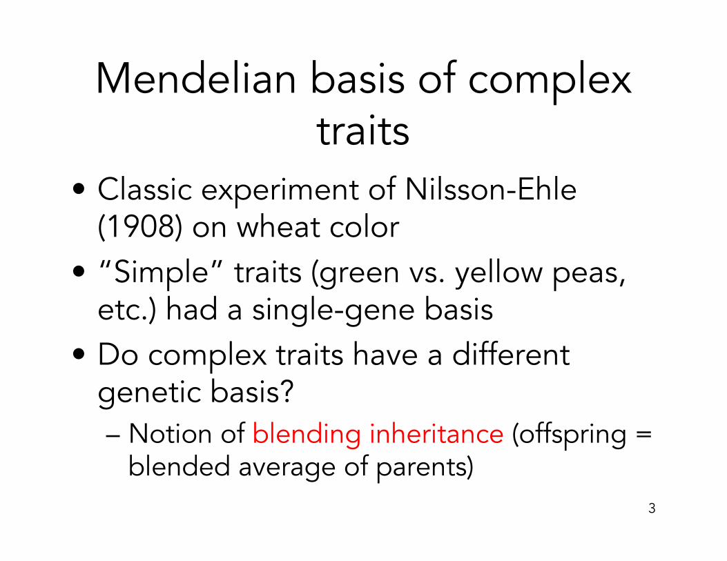
Mendelian basis of complex traits

• Classic experiment of Nilsson-Ehle (1908) on wheat color

• “Simple” traits (green vs. yellow peas, etc.) had a single-gene basis

• Do complex traits have a different genetic basis?– Notion of blending inheritance (offspring =

blended average of parents) 3

4

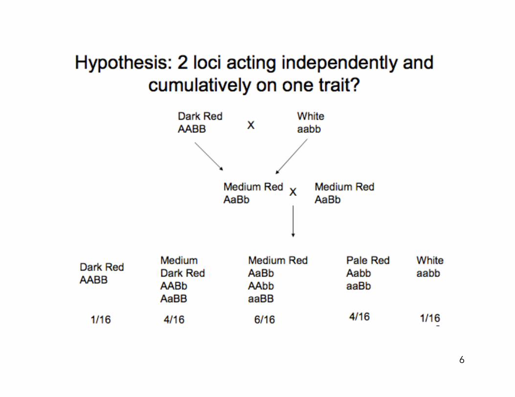
F1 in a cross of dark red pure line x white pureline seems to support blending

However, “outbreak of variation” in the F2rules out blending

6

Stability of the phenotypic distribution over time

8

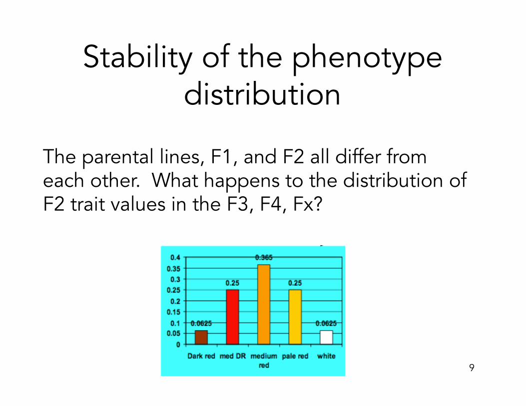
Stability of the phenotype distribution

9

The parental lines, F1, and F2 all differ from each other. What happens to the distribution ofF2 trait values in the F3, F4, Fx?

Case 1: random mating

• Suppose the F2 are randomly mated. What are the genotype frequencies in the following generation?

• These are given by the Hardy-Weinberg theorem.

• If p = freq(A) and q = freq(a), then– freq(AA) = p2

– freq(Aa) = 2pq– freq(aa) = q2

10

• Here freq(A) = freq(a) = ½, and freq(B) = freq(b) = ½. Assuming the A and B loci are unlinked, then independent assortment gives– Freq(dark red) = Freq(AABB) = freq(AA)*freq(BB) =

(1/4) (1/4) = 0.0625– Freq(white) = freq(aabb) = freq(aa)*freq(bb) = 0.0625– Freq(med red) = freq(AAbb or AaBb or aaBB)

• = (1/4)*(1/4) + (1/2)*(1/2) + (1/4)*(1/4) = 0.375

• Hence, the distribution of phenotypes in the F3 is the same as the F2. What about in the F4? F5?

11

Case 2: Inbred lines• Suppose instead that each F2 is used to form

an inbred line, and continually selfed over many generations. What happens to the distribution after complete selfing?

• Now each locus is a homozygote, with Freq(AA) = freq(aa) = freq(BB) = freq(bb) = ½– AABB = dark red (25%)– AAbb, aaBB = medium red (50%)– aabb = white (25%)

12

During selfing• During selfing, an AA or aa line only produces AA /aa.

However, an Aa line has probablity ¼: ½ : ¼ of producing AA : Aa : aa

• Hence, after one generation of selfing– Freq(AA) = Freq(AA | parent AA) + Freq(AA | parent Aa) =

1*(1/4) + (1/4)*(1/2) = 3/8– Freq(aa) = 3/8, freq(Aa) = 1/4– Same for the B locus

• Resulting phenotypic (seed color) frequencies are– Freq(dark red) = Freq(AABB) = freq(AA)*freq(BB) = (3/8)

(3/8) = 0.1406– Freq(white) = freq(aabb) = freq(aa)*freq(bb) = 0.1406– Freq(med red) = freq(AAbb or AaBb or aaBB)

• = (3/8)*(3/8) + (2/8)*(2/8) + (3/8)*(3/8) = 0.34413

Hardy-Weinberg

14

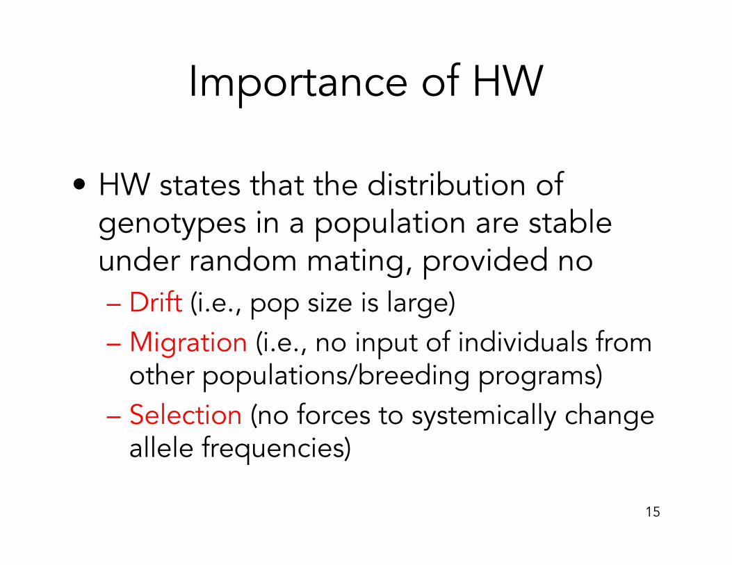
Importance of HW

• HW states that the distribution of genotypes in a population are stable under random mating, provided no– Drift (i.e., pop size is large)– Migration (i.e., no input of individuals from

other populations/breeding programs)– Selection (no forces to systemically change

allele frequencies)

15

Derivation of the Hardy-Weinberg result

• Consider any population, where– Freq(AA) = X– Freq(Aa) = Y– Freq(aa) = Z– freq(A) = p = freq(AA) + (1/2) freq(Aa) = X + ½ Y

• What happens in the next generation from random mating?

16

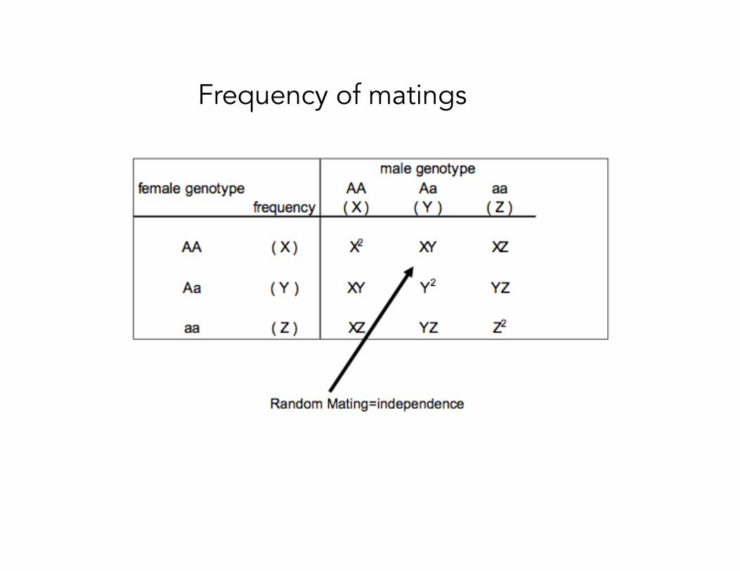
Frequency of matings

Genotype frequencies in next generation

Freq(AA) = 1* X2 + ½*2XY + (1/4) Y2 = (X + ½ Y) 2 = p2.

Freq(aa) = 1* Z2 + ½*2YZ + (1/4) Y2 = (Z + ½ Y) 2 = q2.

What about the next generation?

19

Freq(AA) = 1* p4 + ½*4p3q + (1/4) 4p2q2 = p2 (p+q)2 = p2.

Genotype frequencies unchanged

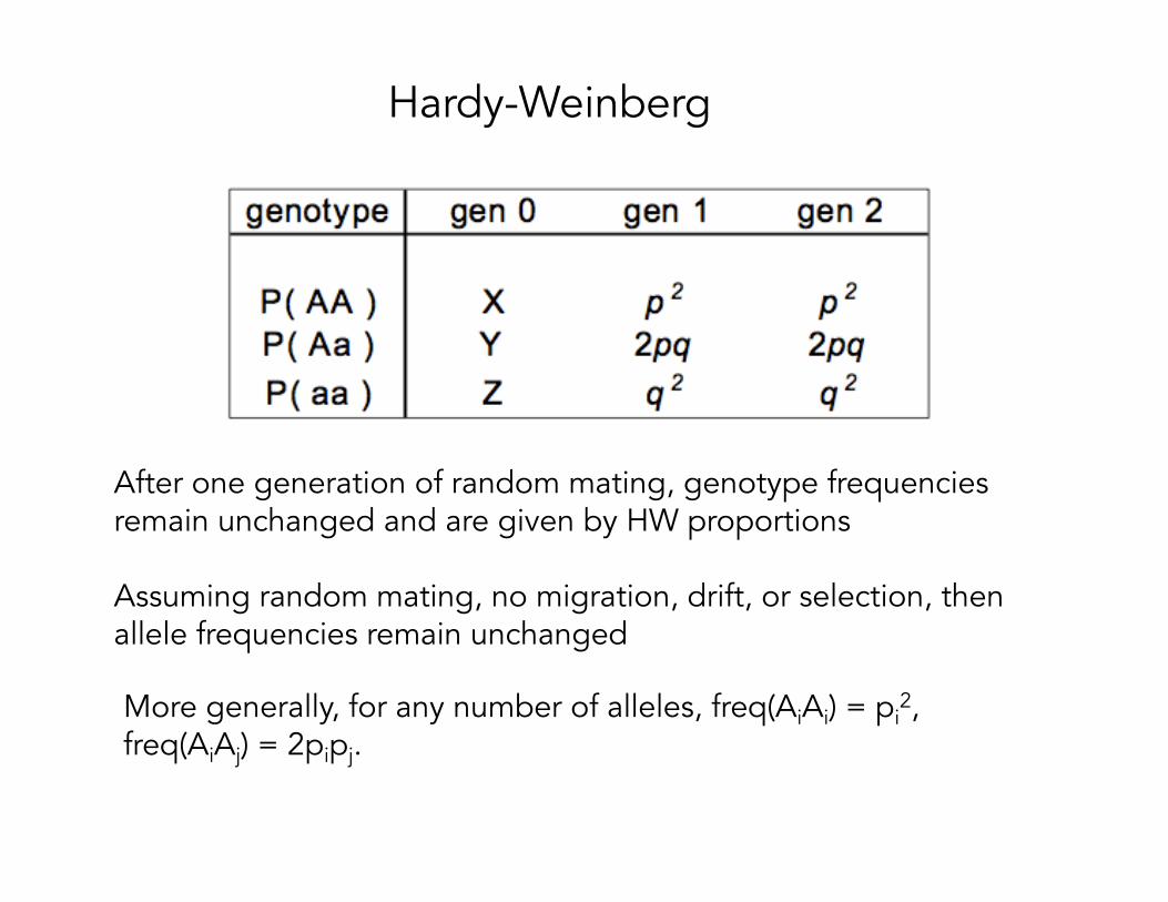
Hardy-Weinberg

After one generation of random mating, genotype frequencies remain unchanged and are given by HW proportions

Assuming random mating, no migration, drift, or selection, thenallele frequencies remain unchanged

More generally, for any number of alleles, freq(AiAi) = pi2,

freq(AiAj) = 2pipj.

Hybridization

• Hardy-Weinberg assumes allele frequencies are the same in both sexes. If not, then after one generation of random mating, the frequencies of autosomal alleles is the same in both sexes, and HW is obtained on the second generation

• Suppose Freq(A in males) = pm, Freq(A in females) = pf. Average allele frequency p = (pm+ pf)/2.

• In generation one,– Freq(AA) = pm* pf which is different from p2 if pm & pf differ– Freq(Aa) = pm (1-pf) + (1-pm) pf

21

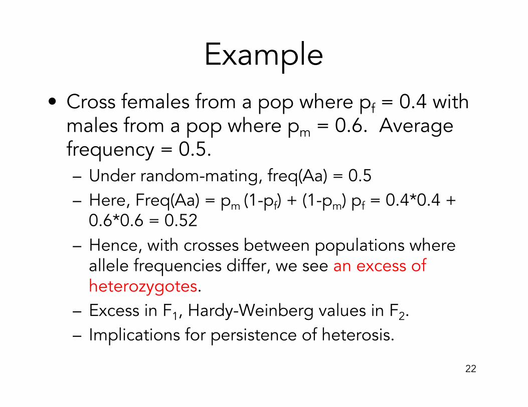
Example• Cross females from a pop where pf = 0.4 with

males from a pop where pm = 0.6. Average frequency = 0.5.– Under random-mating, freq(Aa) = 0.5– Here, Freq(Aa) = pm (1-pf) + (1-pm) pf = 0.4*0.4 +

0.6*0.6 = 0.52– Hence, with crosses between populations where

allele frequencies differ, we see an excess of heterozygotes.

– Excess in F1, Hardy-Weinberg values in F2.– Implications for persistence of heterosis.

22

Crosses vs. synthetics

• In a cross, males and females are always from different populations. Example of nonrandom mating!

• In a synthetic, all individuals are randomly-mated, therefore F2 is in HW

• Example: equal mix of P1 X P2

– In a synthetic, 25% of crosses are P1 X P1, 50% P1 x P2, 25% P2 x P2.

23

Multi-locus Hardy-Weinberg

24

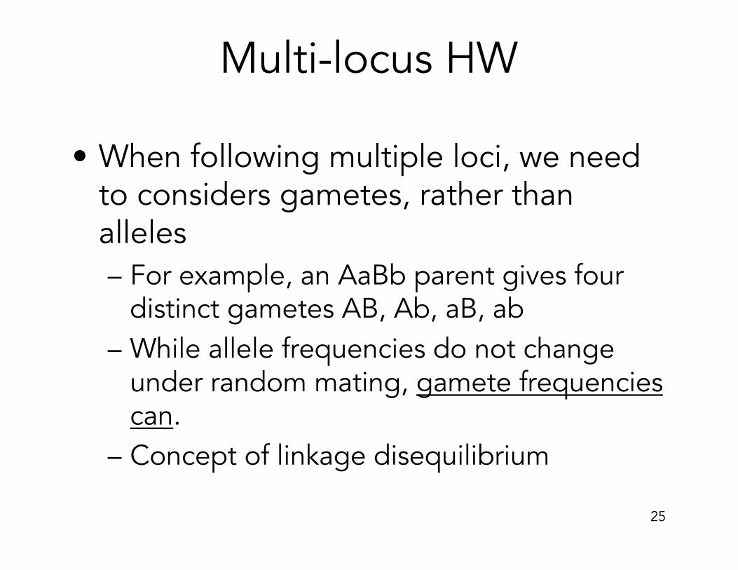
Multi-locus HW

• When following multiple loci, we need to considers gametes, rather than alleles– For example, an AaBb parent gives four

distinct gametes AB, Ab, aB, ab– While allele frequencies do not change

under random mating, gamete frequencies can.

– Concept of linkage disequilibrium

25

Genotypic frequencies under HW

• Under multi-locus HW,– Freq(AABB) = Freq(AA)*Freq(BB)– i.e., can use single-locus HW on each

locus, and then multiply the results

• When D is non-zero (LD is present), cannot use this approach– Rather, must follow gametes

26

27

Linkage Disequilibrium• Under linkage equilibrium, the frequency of gametes

is the product of allele frequencies,– e.g. Freq(AB) = Freq(A)*Freq(B)– A and B are independent of each other

• If the linkage phase of parents in some set or population departs from random (alleles not independent) , linkage disequilibrium (LD) is said to occur

• The amount DAB of disequilibrium for the AB gamete is given by– DAB = Freq(AB) gamete - Freq(A)*Freq(B)– D > 0 implies AB gamete more frequent than expected– D < 0 implies AB less frequent than expected

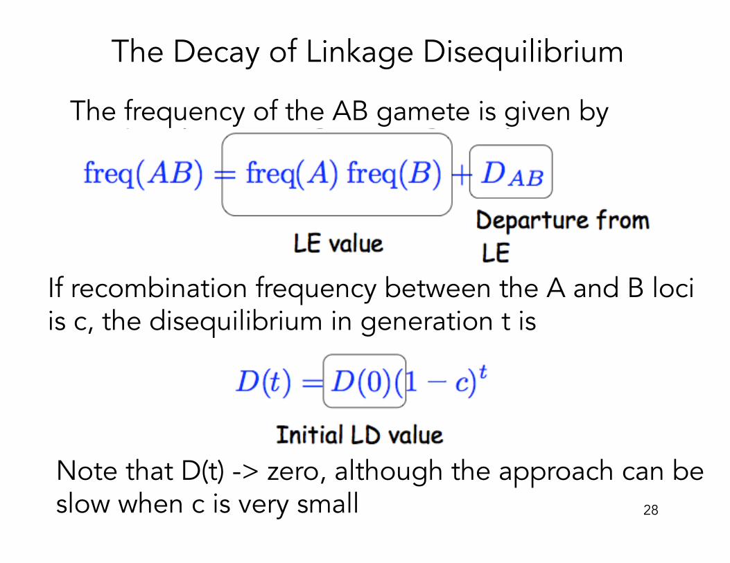
The Decay of Linkage Disequilibrium

The frequency of the AB gamete is given by

If recombination frequency between the A and B lociis c, the disequilibrium in generation t is

Note that D(t) -> zero, although the approach can beslow when c is very small 28

29

Dynamics of D

• Under random mating in a large population, allele frequencies do not change. However, gamete frequencies do if there is any LD

• The amount of LD decays by (1-c) each generation– D(t) = (1-c)t D(0)

• The expected frequency of a gamete (say AB) is– Freq(AB) = Freq(A)*Freq(B) + D– Freq(AB in gen t) = Freq(A)*Freq(B) + (1-c)t D(0)

30

AB/ab

Excess of parentalgametes

AB, ab

linkage

Ab/aB

Excess of parentalgametes

Ab, aB

AB/ab

Excess of parentalgametes

AB, ab

Ab/aB

Excess of parentalgametes

Ab, aB

Pool all gametes: AB, ab, Ab, aB equally frequent

No LD: random distribution of linkage phases

31

AB/ab

Excess of parentalgametes

AB, ab

linkage

AB/ab

Excess of parentalgametes

AB, ab

AB/ab

Excess of parentalgametes

AB, ab

Ab/aB

Excess of parentalgametes

Ab, aB

Pool all gametes: Excess of AB, ab due to an excessof AB/ab parents

With LD, nonrandom distribution of linkage phase

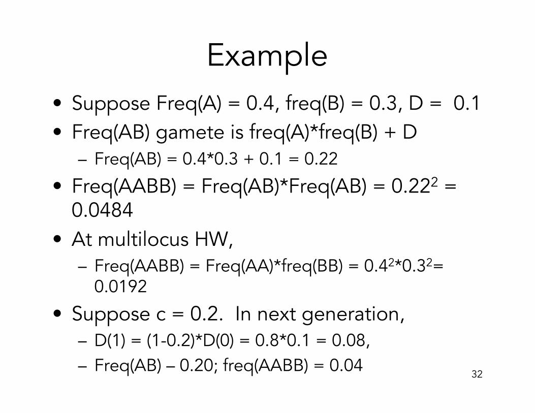
Example• Suppose Freq(A) = 0.4, freq(B) = 0.3, D = 0.1• Freq(AB) gamete is freq(A)*freq(B) + D

– Freq(AB) = 0.4*0.3 + 0.1 = 0.22

• Freq(AABB) = Freq(AB)*Freq(AB) = 0.222 = 0.0484

• At multilocus HW, – Freq(AABB) = Freq(AA)*freq(BB) = 0.42*0.32=

0.0192

• Suppose c = 0.2. In next generation,– D(1) = (1-0.2)*D(0) = 0.8*0.1 = 0.08,– Freq(AB) – 0.20; freq(AABB) = 0.04

32

Population structure

33

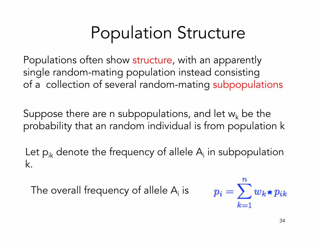
Population StructurePopulations often show structure, with an apparentlysingle random-mating population instead consistingof a collection of several random-mating subpopulations

Suppose there are n subpopulations, and let wk be theprobability that an random individual is from population k

Let pik denote the frequency of allele Ai in subpopulationk.

The overall frequency of allele Ai is

34

The frequency of AiAi in the population is just

Expressed in terms of the population frequency ofAi,

Thus, unless the allele has the same frequency ineach population (Var(pi) = 0), the frequency ofhomozygotes exceeds that predicted from HW

35

Similar logic gives the frequency of heterozygotesas

Hence, when the population shows structure,homozygotes are more commonthan predicted from HW, while heterozygotes canbe more (or less) common than expected under HW,as the covariance could be zero, positive, or negative

36

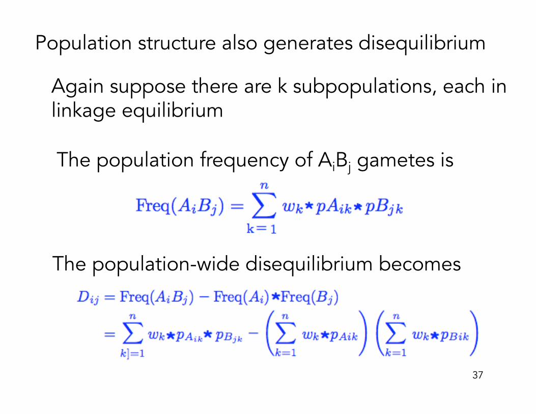
Population structure also generates disequilibrium

Again suppose there are k subpopulations, each inlinkage equilibrium

The population frequency of AiBj gametes is

The population-wide disequilibrium becomes

37

Consider the simplest case of k = 2 populations

Let pi be the frequency of Ai in population 1,pi + di in population 2.

Likewise, let qj be the frequency of Bj in population 1,qj + dj in population 2.

The expected disequilibrium becomes

Here, w1 is the frequency of population 1

38

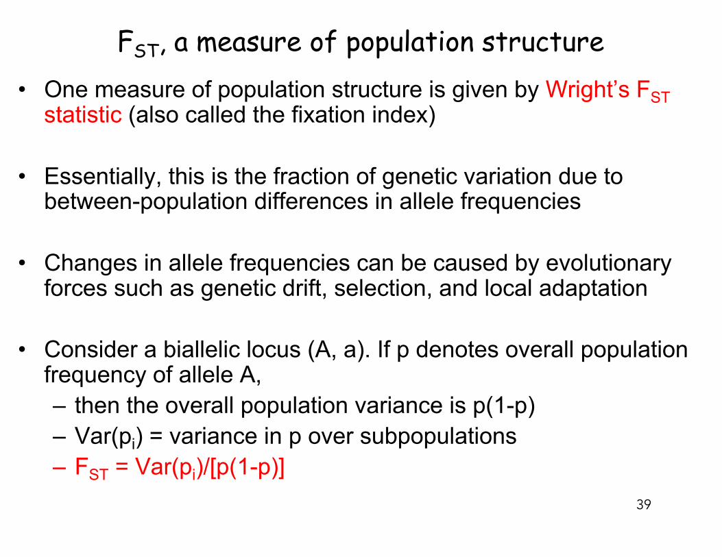
• One measure of population structure is given by Wright’s FSTstatistic (also called the fixation index)

• Essentially, this is the fraction of genetic variation due to between-population differences in allele frequencies

• Changes in allele frequencies can be caused by evolutionary forces such as genetic drift, selection, and local adaptation

• Consider a biallelic locus (A, a). If p denotes overall population frequency of allele A, – then the overall population variance is p(1-p)– Var(pi) = variance in p over subpopulations– FST = Var(pi)/[p(1-p)]

FST, a measure of population structure

39

Population Freq(A)

1 0.1

2 0.6

3 0.2

4 0.7

Assume all subpopulationscontribute equally tothe overall metapopulation

Overall freq(A) = p =(0.1 + 0.6 + 0.2 + 0.7)/4 = 0.4

Var(pi) = E(pi2) - [E(pi)]2 = E(pi

2) - p2

Var(pi) = [(0.12 + 0.62 + 0.22 + 0.72)/4] - 0.42 = 0.065

Total population variance = p(1-p) = 0.4(1-0.4) = 0.24

Hence, FST = Var(pi) /[p(1-p) ] = 0.065/0.24 = 0.27

Example of FST estimation

40

P1

P2

p=0.5q=0.5

p=0.5q=0.5

FST = 0

Graphical example of FST

HomozygousDiploid

No population differentiation 41

Modified from Escalante et al. 2004. Trends Parasitol. 20:388-395

P1

P2

p=0.9q=0.1

p=0.25q=0.75

FST=0.43HomozygousDiploid

Graphical example of FST

Strong population differentiation

42

Modified from Escalante et al. 2004. Trends Parasitol. 20:388-395

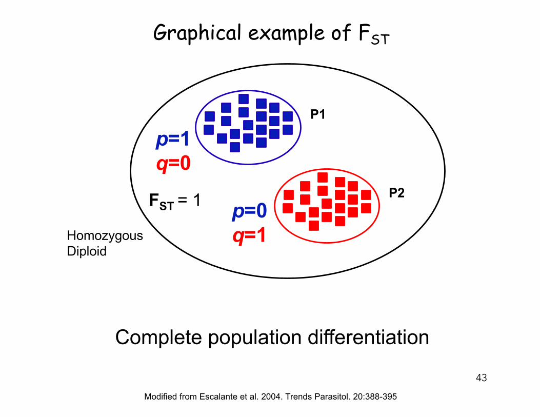
P1

P2

Modified from Escalante et al. 2004. Trends Parasitol. 20:388-395

p=1q=0

p=0q=1

FST = 1

HomozygousDiploid

Complete population differentiation

Graphical example of FST

43

Unrooted neighbor-joining tree based on C.S. Chord (Cavalli-Sforza and Edwards 1967) based on 169 nuclearSSRs. The key relates the color of the line to the chloroplast haplotype based on ORF100 and PS-ID sequences.

Garris et al. 2005. Genetics 169:1631-1638

Rice population structure

*Admixed individuals

FST = 0.25

FST = 0.43

44

Liu et al. 2003. Genetics 165:2117-2128

Phylogenetic tree for 260 inbred lines using the log-transformed proportion of shared alleles distance

Maize population structure

Non-Stiff Stalk

Tropical/Subtropical

Stiff-Stalk

TeosinteFST =0.18

Flint-Garcia et al. 2005. Plant J. 144:1054-1064

FST = 0.22

45

Selection

46

Genotype AA Aa aa

Frequency(before selection)

p2 2p(1-p) (1-p)2

Fitness WAA WAa Waa

Frequency(after selection)

p2 WAA 2p(1-p) WAa (1-p)2Waa

One locus with two alleles

W W W

Wis the mean population fitness, the fitness of an randomindividual, e.g. = E[W]

Where = p2 WAA + 2p(1-p) WAa + (1-p)2WaaW

47

The new frequency p’ of A is just freq(AA after selection) + (1/2) freq(Aa after selection)

The fitness rankings determine the ultimate fateof an allele

If WAA > WAa > Waa, allele A is fixed, a lost

If WAa > WAA, Waa, selection maintains both A & aOverdominant selection

48

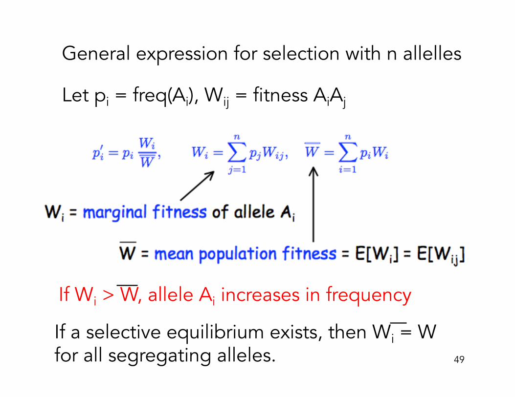
General expression for selection with n allelles

Let pi = freq(Ai), Wij = fitness AiAj

If Wi > W, allele Ai increases in frequency

If a selective equilibrium exists, then Wi = W for all segregating alleles. 49

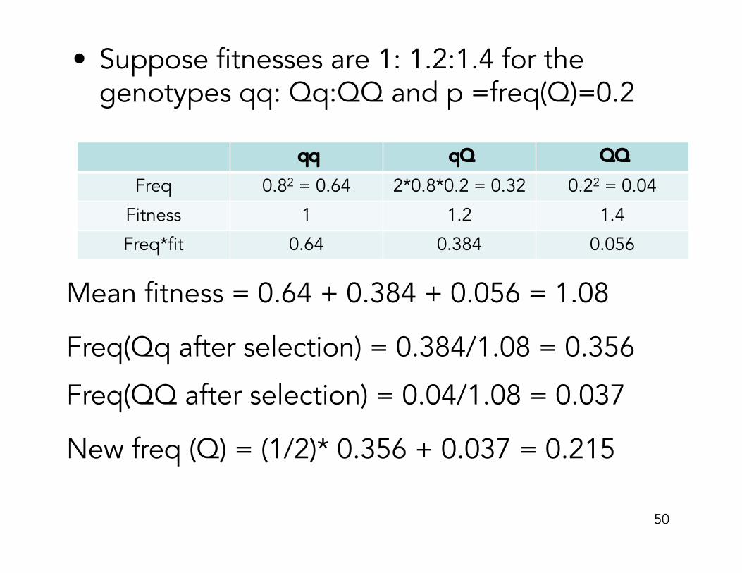
• Suppose fitnesses are 1: 1.2:1.4 for the genotypes qq: Qq:QQ and p =freq(Q)=0.2

50

qq qQ QQ

Freq 0.82 = 0.64 2*0.8*0.2 = 0.32 0.22 = 0.04

Fitness 1 1.2 1.4

Freq*fit 0.64 0.384 0.056

Mean fitness = 0.64 + 0.384 + 0.056 = 1.08

Freq(Qq after selection) = 0.384/1.08 = 0.356

Freq(QQ after selection) = 0.04/1.08 = 0.037

New freq (Q) = (1/2)* 0.356 + 0.037 = 0.215