Lecture # 06 Image Enhancement in Spatial Domain · Lecture # 06 Image Enhancement in Spatial ......
40
Digital Image Processing Lecture # 06 Image Enhancement in Spatial Domain Autumn 2012
Transcript of Lecture # 06 Image Enhancement in Spatial Domain · Lecture # 06 Image Enhancement in Spatial ......

Digital Image Processing
Lecture # 06
Image Enhancement in Spatial
Domain
Autumn 2012

Digital Image Processing Lecture # 6 2
Limitations of Point Operations
► They don’t know where they are in an image
► They don’t know anything about their neighbors
► Most image features (edges, textures, etc) involve a spatial neighborhood of pixels
► If we want to enhance or manipulate these features, we need to go beyond point operations

Digital Image Processing Lecture # 6 3
What Point Operations Can’t Do
►Blurring / Smoothing

Digital Image Processing Lecture # 6 4
What Point Operations Can’t Do
►Sharpening

Digital Image Processing Lecture # 6 5
Spatial Filtering
• Filter term in “Digital image processing” is referred to the subimage
• There are others term to call subimage such as mask, kernel, template, or window
• The value in a filter subimage are referred as coefficients, rather than pixels.
• The concept of filtering has its roots in the use of the Fourier transform for signal processing in the so-called frequency domain.
• Spatial filtering term is the filtering operations that are performed directly on the pixels of an image.

Digital Image Processing Lecture # 6 6
Spatial Filtering
A spatial filter consists of (a) a neighborhood, and (b) a predefined operation
Linear spatial filtering of an image of size MxN with a filter of size mxn is given by the expression
( , ) ( , ) ( , )a b
s a t b
g x y w s t f x s y t

Digital Image Processing Lecture # 6 7
Spatial Filtering
Digital Image Processing Lecture # 6 8
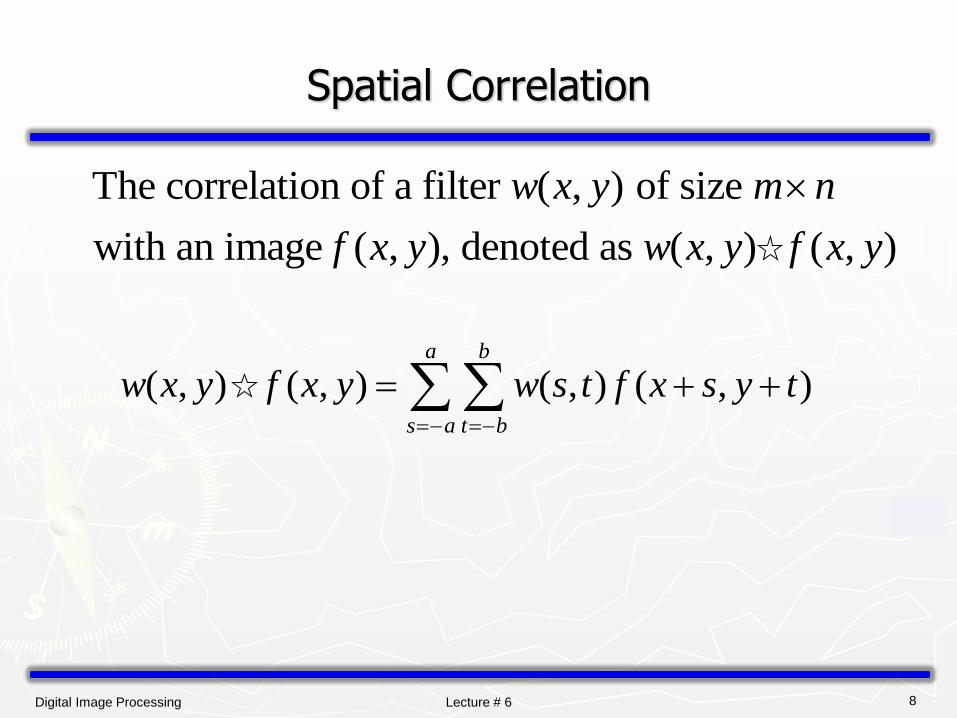
Spatial Correlation
The correlation of a filter ( , ) of size
with an image ( , ), denoted as ( , ) ( , )
w x y m n
f x y w x y f x y
( , ) ( , ) ( , ) ( , )a b
s a t b
w x y f x y w s t f x s y t
Digital Image Processing Lecture # 6 9
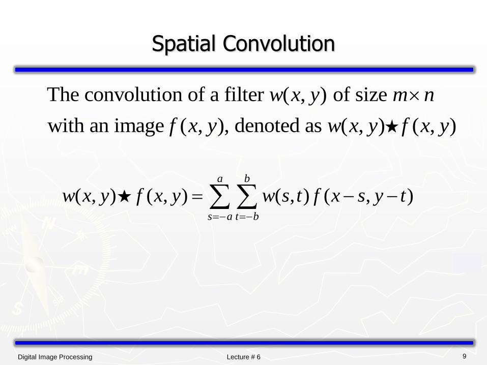
Spatial Convolution
The convolution of a filter ( , ) of size
with an image ( , ), denoted as ( , ) ( , )
w x y m n
f x y w x y f x y
( , ) ( , ) ( , ) ( , )a b
s a t b
w x y f x y w s t f x s y t

Digital Image Processing Lecture # 6 10
Digital Image Processing Lecture # 6 11
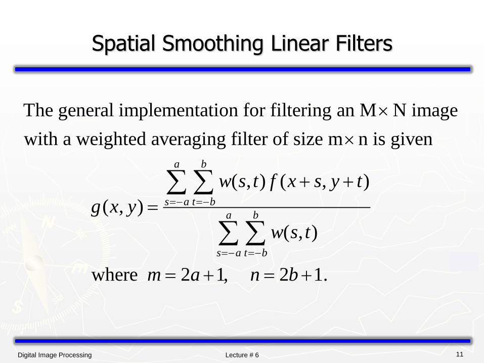
Spatial Smoothing Linear Filters
The general implementation for filtering an M N image
with a weighted averaging filter of size m n is given
( , ) ( , )
( , )
( , )
where 2 1
a b
s a t b
a b
s a t b
w s t f x s y t
g x y
w s t
m a
, 2 1.n b

Digital Image Processing Lecture # 6 12
Smoothing Spatial Filters
► used for blurring and for noise reduction
► blurring is used in preprocessing steps, such as
removal of small details from an image prior to object extraction
bridging of small gaps in lines or curves
► noise reduction can be accomplished by blurring with a linear filter and also by a nonlinear filter
► replacing the value of every pixel in an image by the average of the gray levels in the neighborhood will reduce the “sharp” transitions in gray levels. sharp transitions
► random noise in the image
► edges of objects in the image
► thus, smoothing can reduce noises (desirable) and blur edges (undesirable)

Digital Image Processing Lecture # 6 13
Two Smoothing Averaging Filter Masks

Digital Image Processing Lecture # 6 14

Digital Image Processing Lecture # 6 15
Example: Gross Representation of Objects

Digital Image Processing Lecture # 6 16
Example: Smoothing Filter
[3x3] [5x5] [7x7]
Original Image

Digital Image Processing Lecture # 6 17
Order-statistic (Nonlinear) Filters
— Nonlinear
— Based on ordering (ranking) the pixels contained in the filter mask
— Replacing the value of the center pixel with the value determined by the ranking result
E.g., median filter, max filter, min filter

Digital Image Processing Lecture # 6 18
Median Filters
► replaces the value of a pixel by the median of the gray levels in the neighborhood of that pixel (the original value of the pixel is included in the computation of the median)
► quite popular because for certain types of random noise (impulse noise salt and pepper noise) , they provide excellent noise-reduction capabilities, with considering less blurring than linear smoothing filters of similar size.

Digital Image Processing Lecture # 6 19
Example: Use of Median Filtering for Noise Reduction

Digital Image Processing Lecture # 6 20
Sharpening Spatial Filters
► Foundation
► Laplacian Operator
► Unsharp Masking and Highboost Filtering
► Using First-Order Derivatives for Nonlinear Image Sharpening — The Gradient

Digital Image Processing Lecture # 6 21
Sharpening Spatial Filters
► to highlight fine detail in an image
► or to enhance detail that has been blurred, either in error or as a natural effect of a particular method of image acquisition.
► Blurring Vs. Sharpening
as we know that blurring can be done in spatial domain by pixel averaging in a neighbors
since averaging is analogous to integration
thus, we can guess that the sharpening must be accomplished by spatial differentiation.

Digital Image Processing Lecture # 6 22
Derivative operator
► the strength of the response of a derivative operator is proportional to the degree of discontinuity of the image at the point at which the operator is applied.
► thus, image differentiation
enhances edges and other discontinuities (noise)
deemphasizes area with slowly varying gray-level values.

Digital Image Processing Lecture # 6 23
Sharpening Spatial Filters: Foundation
► The first-order derivative of a one-dimensional function f(x) is the difference
► The second-order derivative of f(x) as the difference
( 1) ( )f
f x f xx
2
2( 1) ( 1) 2 ( )
ff x f x f x
x

Digital Image Processing Lecture # 6 24
First and Second Derivative
► First Derivative
Must be zero in flat segments
Must be nonzero at the onset of a gray-level step or ramp; and
Must be nonzero along ramps.
► Second Derivative
Must be zero in flat areas;
Must be nonzero at the onset and end of a gray-level step or ramp;
Must be zero along ramps of constant slope

Digital Image Processing Lecture # 6 25

Digital Image Processing Lecture # 6 26
Sharpening Spatial Filters: Laplace Operator
The second-order isotropic derivative operator is the Laplacian for a function (image) f(x,y)
2 22
2 2
f ff
x y
2
2( 1, ) ( 1, ) 2 ( , )
ff x y f x y f x y
x
2
2( , 1) ( , 1) 2 ( , )
ff x y f x y f x y
y
2 ( 1, ) ( 1, ) ( , 1) ( , 1)
- 4 ( , )
f f x y f x y f x y f x y
f x y

Digital Image Processing Lecture # 6 27
Sharpening Spatial Filters: Laplace Operator

Digital Image Processing Lecture # 6 28
Sharpening Spatial Filters: Laplace Operator
Image sharpening in the way of using the Laplacian:
2
2
( , ) ( , ) ( , )
where,
( , ) is input image,
( , ) is sharpenend images,
-1 if ( , ) corresponding to Fig. 3.37(a) or (b)
and 1 if either of the other two filters is us
g x y f x y c f x y
f x y
g x y
c f x y
c
ed.

Digital Image Processing Lecture # 6 29

Digital Image Processing Lecture # 6 30
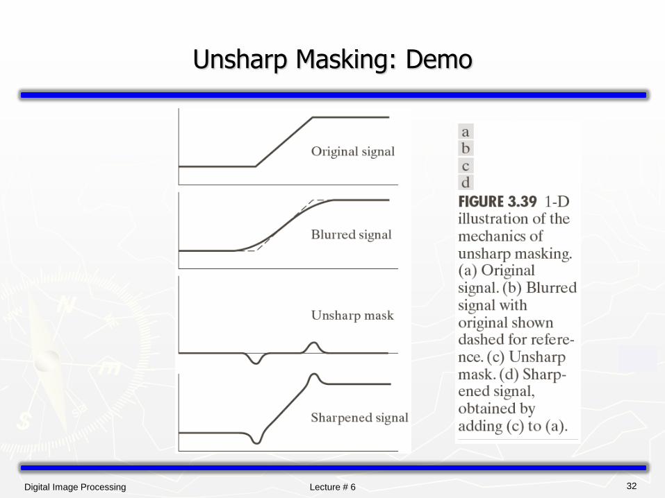
Unsharp Masking and Highboost Filtering
► Unsharp masking
Sharpen images consists of subtracting an unsharp (smoothed) version of an image from the original image
e.g., printing and publishing industry
► Steps
1. Blur the original image
2. Subtract the blurred image from the original
3. Add the mask to the original

Digital Image Processing Lecture # 6 31
Unsharp Masking and Highboost Filtering
Let ( , ) denote the blurred image, unsharp masking is
( , ) ( , ) ( , )
Then add a weighted portion of the mask back to the original
( , ) ( , ) * ( , )
mask
mask
f x y
g x y f x y f x y
g x y f x y k g x y
0k
when 1, the process is referred to as highboost filtering.k
Digital Image Processing Lecture # 6 32
Unsharp Masking: Demo

Digital Image Processing Lecture # 6 33
Unsharp Masking and Highboost Filtering: Example
Digital Image Processing Lecture # 6 34
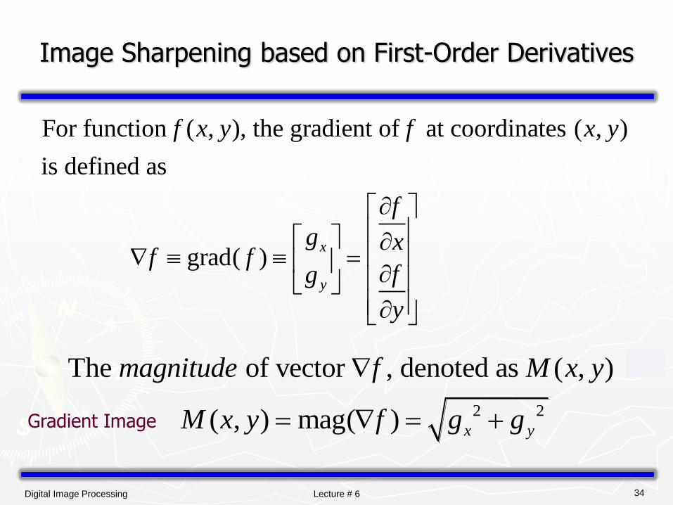
Image Sharpening based on First-Order Derivatives
For function ( , ), the gradient of at coordinates ( , )
is defined as
grad( )x
y
f x y f x y
f
g xf f
fg
y
2 2
The of vector , denoted as ( , )
( , ) mag( ) x y
magnitude f M x y
M x y f g g
Gradient Image

Digital Image Processing Lecture # 6 35
Image Sharpening based on First-Order Derivatives
2 2
The of vector , denoted as ( , )
( , ) mag( ) x y
magnitude f M x y
M x y f g g
( , ) | | | |x yM x y g g
z1 z2 z3
z4 z5 z6
z7 z8 z9
8 5 6 5( , ) | | | |M x y z z z z
Digital Image Processing Lecture # 6 36
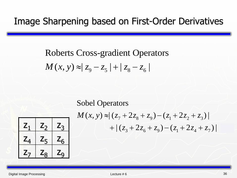
Image Sharpening based on First-Order Derivatives
z1 z2 z3
z4 z5 z6
z7 z8 z9
9 5 8 6
Roberts Cross-gradient Operators
( , ) | | | |M x y z z z z
7 8 9 1 2 3
3 6 9 1 4 7
Sobel Operators
( , ) | ( 2 ) ( 2 ) |
| ( 2 ) ( 2 ) |
M x y z z z z z z
z z z z z z

Digital Image Processing Lecture # 6 37
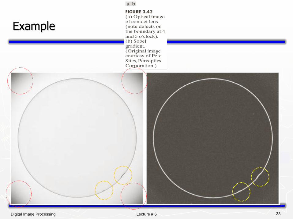
Image Sharpening based on First-Order Derivatives
Digital Image Processing Lecture # 6 38
Example

Digital Image Processing Lecture # 6 39
Example: Combining Spatial Enhancement Methods Goal: Enhance the image by sharpening it and by bringing out more of the skeletal detail

Digital Image Processing Lecture # 6 40
Example: Combining Spatial Enhancement Methods Goal: Enhance the image by sharpening it and by bringing out more of the skeletal detail