Learning with Probabilistic Featuresfor Improved Pipeline Models

Razvan C. BunescuElectrical Engineering and Computer Science

Ohio UniversityAthens, OH

bunescu@ohio.edu

EMNLP, October 2008

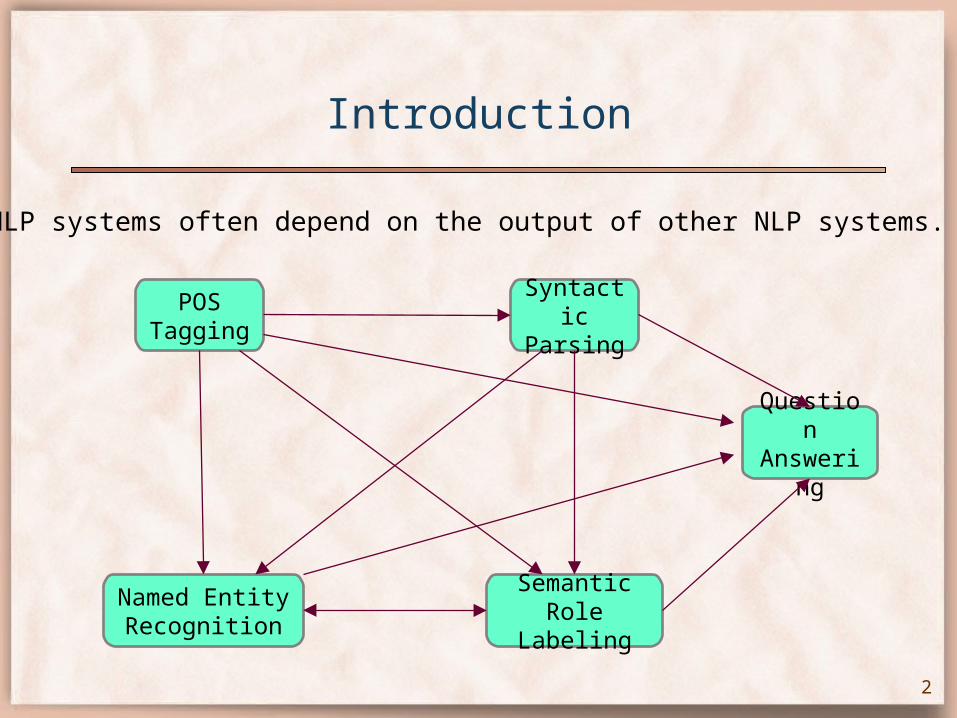
Introduction

2

Syntactic Parsing

POS Tagging

Semantic Role Labeling

Named Entity Recognition

Question Answering

• NLP systems often depend on the output of other NLP systems.

Traditional Pipeline Model: M1

3

Syntactic Parsing

POS Tagging

x )(ˆ, xzx )(ˆ xy

)|(maxarg)(ˆ

))(ˆ,,(maxarg)(ˆ

)(

)(

xzpxz

xzyxwxy

xZz

xYy

• The best annotation from one stage is used in subsequent stages.

• Problem: Errors propagate between pipeline stages!

Probabilistic Pipeline Model: M2

4

Syntactic Parsing

POS Tagging

x )(, xZx )(ˆ xy

)(

)(

),,()|(),(

),(maxarg)(ˆ

xZz

xYy

zyxxzpyx

yxwxy

• All possible annotationsfrom one stage are used in subsequent stages.

• Problem: Z(x) has exponential cardinality!

probabilistic features

Probabilistic Pipeline Model: M2

5

• When original i‘s are count features, it can be shown that:

)(

),,()|(),(xZz

ii zyxxzpyx

nii yxyx ..1)],([),( • Feature-wise formulation:

))(,,()~,~,~(

)|~( ),(xZyxFzyx

i

i

xzpyx

An instance of feature i , i.e. the actual evidence used from example (x,y,z).

Probabilistic Pipeline Model

6

• When original i‘s are count features, it can be shown that:

)(

),,()|(),(xZz

ii zyxxzpyx

nii yxyx ..1)],([),(

))(,,()~,~,~(

)|~( ),(xZyxFzyx

i

i

xzpyx

• Feature-wise formulation:

The set of all instances of feature i in (x,y,z), across all annotations zZ(x).

Probabilistic Pipeline Model

7

• When original i‘s are count features, it can be shown that:

)(

),,()|(),(xZz

ii zyxxzpyx

nii yxyx ..1)],([),(

))(,,()~,~,~(

)|~( ),(xZyxFzyx

i

i

xzpyx

• Feature-wise formulation:

Example: POS Dependency Parsing

8

The1 sailors2 mistakenly3 thought4 there5 must6 be7 diamonds8 in9 the10 soil11

RB VBD

y~

z~

)|~( xzp

• Feature i RB VBD

• The set of feature instances Fi is:

0.91

Example: POS Dependency Parsing

9

The1 sailors2 mistakenly3 thought4 there5 must6 be7 diamonds8 in9 the10 soil11

RB VBD

y~

z~

)|~( xzp

• Feature i RB VBD

• The set of feature instances Fi is:

0.01

RB VBD

0.91

Example: POS Dependency Parsing

10

The1 sailors2 mistakenly3 thought4 there5 must6 be7 diamonds8 in9 the10 soil11

RB VBD

y~

z~

)|~( xzp

• Feature i RB VBD

• The set of feature instances Fi is:

0.1

RB VBD

0.01

RB VBD

0.91

Example: POS Dependency Parsing

11

The1 sailors2 mistakenly3 thought4 there5 must6 be7 diamonds8 in9 the10 soil11

RB VBD

y~

z~

)|~( xzp

• Feature i RB VBD

• The set of feature instances Fi is:

0.001

RB VBD

0.1

RB VBD

0.01

RB VBD

0.91

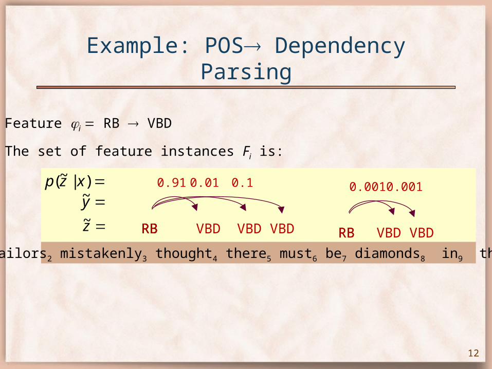
Example: POS Dependency Parsing

12

The1 sailors2 mistakenly3 thought4 there5 must6 be7 diamonds8 in9 the10 soil11

RB VBD

y~

z~

)|~( xzp

• Feature i RB VBD

• The set of feature instances Fi is:

0.001

RB VBD

0.001

RB VBD

0.1

RB VBD

0.01

RB VBD

0.91

Example: POS Dependency Parsing

13

The1 sailors2 mistakenly3 thought4 there5 must6 be7 diamonds8 in9 the10 soil11

RB VBD

y~

z~

)|~( xzp

• Feature i RB VBD

• The set of feature instances Fi is:

0.002

RB VBD

0.001

RB VBD

0.001

RB VBD

0.1

RB VBD

0.01

RB VBD

0.91

Example: POS Dependency Parsing

14

The1 sailors2 mistakenly3 thought4 there5 must6 be7 diamonds8 in9 the10 soil11

y~

z~

)|~( xzp

• Feature i RB VBD

• The set of feature instances Fi is:

N(N-1) feature instances in Fi .

RB VBD

0.002

RB VBD

0.001

RB VBD

0.001

RB VBD

0.1

RB VBD

0.01

RB VBD

0.91

……

Example: POS Dependency Parsing

15

1) Feature i RB VBD uses a limited amount of evidence:

the set of feature instances Fi has cardinality N(N-1).

2)

computing takes O(N|P|2) time using a constrained version of

the forward-backward algorithm:

Therefore, computing i takes O(N3|P|2) time.

)|~( xzp

)|VBD ,RB( is )|~( xttpxzp ji

))(,,()~,~,~(

)|~( ),(xZyxFzyx

i

i

xzpyx

Probabilistic Pipeline Model: M2

16

nii yxyx ..1)],([),(

))(,,()~,~,~(

)|~( ),(xZyxFzyx

i

i

xzpyx

),(maxarg)(ˆ)(

yxwxyxYy

Syntactic Parsing

POS Tagging

x )(, xZx )(ˆ xy

• All possible annotations from one stage are used in subsequent stages.

polynomial time

• In general, the time complexity of computing i depends on the complexity of the evidence used by feature i. z~

Probabilistic Pipeline Model: M3

17

nii yxyx ..1)],([),(

))(ˆ,,()~,~,~(

)|~( ),(xzyxFzyx

i

i

xzpyx

),(maxarg)(ˆ)(

yxwxyxYy

Syntactic Parsing

POS Tagging

x )(ˆ, xzx )(ˆ xy

• The best annotationfrom one stage is used in subsequent stages, together with its probabilistic confidence:

Probabilistic Pipeline Model: M3

18

nii yxyx ..1)],([),(

))(ˆ,,()~,~,~(

)|~( ),(xzyxFzyx

i

i

xzpyx

),(maxarg)(ˆ)(

yxwxyxYy

Syntactic Parsing

POS Tagging

x )(ˆ, xzx )(ˆ xy

• The best annotationfrom one stage is used in subsequent stages, together with its probabilistic confidence:

The set of instances of feature i using only the best annotation z

Probabilistic Pipeline Model: M3

• Like the traditional pipeline model M1, except that it uses the probabilistic confidence values associated with annotation features.

• More efficient than M2, but less accurate.

• Example: POS Dependency Parsing– shows features generated by template ti tj and their probabilities.

19

The1 sailors2 mistakenly3 thought4 there5 must6 be7 diamonds8 in9 the10 soil11

DT1 NNS2 RB3 VBD4 EX5 MD6 VB7 NNS8 IN9 DT10 NN11

x:

y::z

0.98 0.910.85

0.900.95

0.92

0.970.97

0.98

0.81

Probabilistic Pipeline Models

20

nii yxyx ..1)],([),(

))(ˆ,,()~,~,~(

)|~( ),(xzyxFzyx

i

i

xzpyx

),(maxarg)(ˆ)(

yxwxyxYy

nii yxyx ..1)],([),(

))(,,()~,~,~(

)|~( ),(xZyxFzyx

i

i

xzpyx

),(maxarg)(ˆ)(

yxwxyxYy

Model M2 Model M3

Two Applications

1) Dependency Parsing

2) Named Entity Recognition

21

Syntactic Parsing

POS Tagging

x )(xz )(ˆ xy

Syntactic Parsing

POS Tagging

x

)(1 xz

Named Entity Recognition

)(ˆ xy

)(2 xz

)(1 xz

1) Dependency Parsing

• Use MSTParser [McDonald et al. 2005]:– The score of a dependency tree the sum of the edge scores:

– Feature templates use words and POS tags at positions u and v and their neighbors u 1 and v 1.

• Use CRF [Lafferty et al. 2001] POS tagger:– Compute probabilistic features using a constrained

forward-backward procedure.– Example: feature titj has probability p(ti, tj)

• constrain the state transitions to pass through tags ti and tj.

22

yvu

vuxyx ),(),(

)|~( xzp

1) Dependency Parsing

• Two approximations of model M2:– Model M2’:

• Consider POS tags independent:– p(ti RB,tj VBD|x) p(ti RB|x) p(tj VBD|x)

• Ignore tags with low marginal probability:– p(ti) 1/(|P|)

– Model M2”:

• Like M2’, but use constrained forward-backward to compute marginal probabilities when the tag chunks are less than 4 tokens apart.

23

1) Dependency Parsing: Results

• Train MSTParser on sections 2-21 of Pen WSJ Treebank using gold POS tagging.

• Test MST Parser on section 23, using POS tags from CRF tagger.

• Absolute error reduction of “only” 0.19% :– But POS tagger has a very high accuracy of 96.25%.

• Expect more substantial improvement when upstream stages in the pipeline are less accurate.

24

M1 M2 ’(1) M2 ’(2) M2 ’(4) M2 ”(4)

88.51 88.66 88.67 88.67 88.70

2) Named Entity Recognition

• Model NER as a sequence tagging problem using CRFs:

25

The1 sailors2 mistakenly3 thought4 there5 must6 be7 diamonds8 in9 the10 soil11

DT1 NNS2 RB3 VBD4 EX5 MD6 VB7 NNS8 IN9 DT10 NN11

x:

z2:z1:

y: O I O O O O O O O O O

• Flat features: unigram, bigram and trigram that extend either left or right: sailors, the sailors, sailors RB, sailors RB thought…

• Tree features: unigram, bigram and trigram that extend in any direction in the undirected dependency tree:- sailors thought, sailors thought RB, NNS thought RB, …

Named Entity Recognition: Model M2

26

Syntactic Parsing

POS Tagging

x

)(1 xz

Named Entity Recognition

)(ˆ xy

)(2 xz

)(1 xz

)|~(),~|~()|~,~()|~( 11221 xzpxzzpxzzpxzp

)|,(),,|342()|~( 3232 xRBNNSpxRBNNSpxzp

• Probabilistic features:

• Example feature NNS2 thought4 RB3:

Named Entity Recognition: Model M3’

• M3’ is an approximation of M3 in which confidence scores are computed as follows:– Consider POS tagging and dependency parsing independent.– Consider POS tags independent.– Consider dependency arcs independent.– Example feature NNS2 thought4 RB3:

• Need to compute marginals p(uv|x).

27

)|43()|42()|~(

)|()|()|~(

)|~()|~()|~(

2

321

21

xpxpxzp

xRBtpxNNStpxzp

xzpxzpxzp

Probabilistic Dependency Features

• To compute probabilistic POS features, we used a constrained version of the forward-backward algorithm.

• To compute probabilistic dependency features, we use a constrained version of Eisner’s algorithm:– Compute normalized scores n(uv | x) using the softmax function:

– Transform scores n(uv|x) into probabilities p(uv|x) using isotonic regression [Zadrozny & Elkan, 2002].

28

)(

),(

),(

),(

),(

xYy

yxs

yvuxYy

yxs

e

e

vuxn

Named Entity Recognition: Results

• Implemented the CRF models in MALLET [McCallum, 2002]• Trained and tested on the standard split from the ACE 2002 + 2003

corpus (674 training, 97 testing).

• POS tagger and MSTParser were trained on sections 2-21 of WSJ Treebank– Isotonic regression for MSTParser on section 23.

29

Model Tree Flat Tree+Flat

M3’ 76.78 77.02 77.96

M1 74.38 76.53 77.02

Area under PR curve

Named Entity Recognition: Results

30

• M3’ (probabilistic) vs. M1 (traditional) using tree features:

Conclusions & Related Work

• A general method for improving the communication between consecutive stages in pipeline models:– based on computing expectations for count features.

• an efective method for associating probabilities with output substructures.

– adds polynomial time complexity to pipeline whenever the inference step at each stage is done in polynomial time.

• Can be seen as complementary to the sampling approach of [Finkel et al. 2006]:– approximate vs. exact in polynomial time.– used in testing vs. used in training and testing.

31

Future Work

1) Try full model M2 / its approximation M2’ on NER.

2) Extend model to pipeline graphs containing cycles.

32

Questions?

33