Learning to Recognize Shadows in Monochromatic Natural Images

Jiejie Zhu, Kegan G.G. Samuel, Syed Z. Masood, Marshall F. TappenUniversity of Central Florida

School of Electrical Engineering and Computer Science, Orlando, FLjjzhu,kegan,smasood,mtappen@eecs.ucf.edu

Abstract

This paper addresses the problem of recognizing shad-ows from monochromatic natural images. Without chro-matic information, shadow classification is very challeng-ing because the invariant color cues are unavailable. Nat-ural scenes make this problem even harder because of am-biguity from many near black objects. We propose to useboth shadow-variant and shadow-invariant cues from illu-mination, textural and odd order derivative characteristics.Such features are used to train a classifier from boostinga decision tree and integrated into a Conditional randomField, which can enforce local consistency over pixel la-bels. The proposed approach is evaluated using both quali-tative and quantitative results based on a novel database ofhand-labeled shadows. Our results show shadowed areas ofan image can be identified using proposed monochromaticcues.

1. Introduction

Shadows are one of the most noticeable effects on ascene’s illumination. While they can provide useful cuesregarding scene properties such as object size, shape, andmovement [14], they can also complicate recognition tasks,such as feature detection, object recognition and scene pars-ing. In recent years, multiple groups have proposed meth-ods on removing the effects of illumination from an im-age [4, 32, 27, 24] and have also proposed approaches thatspecifically focus on removing shadows [8, 2, 25, 3].

In systems that focus on shadows, color is the primarycue used to identify the shadow. Finlaysonet al. [8] lo-cated the shadows using an invariant color model. Shor andLischinski [25] propagated the shadows using a color-basedregion growing method. Salvadoret al. [23] used invariantcolor features to segment cast shadows. Levine [15] andArevalo [3] both studied the color ratios across boundariesto assist shadow recognition. A number of other approacheshave also focused on shadow detection using color-relatedmotion cues [21, 19, 31, 16, 12].

These color-assisted systems rely on the assumption that

(a) Diffuse (b) Specularity (c) Self-shading

Figure 1. Ambiguity of shadow recognition in monochromatic do-main. The diffuse object (swing) in (a) and the specular object(car) in (b) both have a dark albedo. The trees in the aerial image(c) appear black because of self-shading. Such objects are verydifficult to be separated from shadows which are also relativelydark.

the chromatic appearance of image regions does not changeacross shadow boundaries, while the intensity componentof a pixel’s color does. Such approaches work well givencolor images where the surfaces are still discernible insidethe shadow.

In this paper, we focus on detecting shadows in a sin-gle monochromatic image. This problem is challenging be-cause images in the monochromatic domain tend to havemany objects appear black or near black (see in Figure1). These objects complicate shadow recognition as shad-ows are expected to be relatively dark. In addition, naturalscenes make it even harder because of their complex illu-mination conditions. We must be very conservative whenlabeling a pixel as shadow in these situations, because non-shadow pixels are similar to shadow pixels if chromatic cuesare unavailable.

Our work on this problem is motivated by two main fac-tors. The first motivation is that color may not be avail-able in all types of sensors, such as sensors tuned to specificspectra, sensors designed for specific usages such as aerial,satellite, celestial images and images captured from veryhigh dynamic scenes. Our second motivation is to under-stand how monochromatic cues can be explored and used torecognize shadows. While chromatic variations have beenshown to aid in the recognition of shadows, humans are stillable to find shadows in monochromatic images [10]. Work-ing with monochromatic images makes it necessary to in-vestigate the usual characteristics of shadows.

1

We present a learning-based approach for detectingshadows in a single monochromatic image. Our approach isnovel, with respect to other shadow detection and removalmethods, in that our system is trained and evaluated on adatabase of natural images and uses both shadow-variantand shadow-invariant cues.

This data-driven approach is unique because previouslearning-based approaches have been evaluated on limiteddatasets, such as highways, parking lots or indoor office en-vironments [20]. Gray-scale cues have also been proposedto remove general illumination effects [4, 32, 27], but thesesystems are limited by their reliance on either syntheticallygenerated training data or data from specialized environ-ments, such as the crumpled paper images from [29]. Inaddition, these systems mainly focus on the variant cues;it will be shown that improved recognition rates can beachieved by combining them with invariant cues.

Our approach is based on boosted decision tree classi-fiers and integrated into a Conditional Random Field (CRF).To make it possible to learn the CRF parameters, we use aMarkov Random Field (MRF) model designed for labeling[28]. The various design decisions in this system, such asoptimization method and feature choice, will be evaluatedas part of the experiments. Our results show that shadows inmonochromatic images can be found with color-free cues.

The contributions of this paper include: (1) an approachfor shadow recognition in monochromatic natural images;(2) several useful features to locate shadows from naturalscenes; (3) a database of monochromatic shadows availableto the public. We also present a convenient implementationof parallel training to efficiently learn the CRF parameters.1.1. Monochromatic Shadow Dataset

We have constructed a database consisting of245 im-ages. In each image, the shadows have been hand-labeled atthe pixel level with two people validating the labeled shad-ows. In this database, 117 of the images were collected bythe authors in a variety of outdoor environments, such as oncampus and downtown areas,etc. To ensure a wide varietyof lighting conditions, we also collect images at differenttimes throughout the day. The dataset includes additional74 257x257 sized aerial images from the Overhead ImageryResearch Dataset (OIRDS) [26] and another54 640x480sized images from LabelMe dataset [22]. Figure 2 showsseveral images with shadows from the dataset.

The camera we used to capture part of the images in thedatabase is a Canon Digital Rebel XTi. The camera modelused for the shadow images from the Labelme database andfrom the OIRDS database are not reported.

2. Feature Extraction

Given a single monochromatic natural image, we wouldlike to identify those pixels that are associated with shad-ows. Without color information, the features in our ex-

Figure 2.Example of shadows in the dataset. The images captured bythe authors are linearly transformed from raw format to TIF format. Theimages from LableMe are in JPG format. The images from OIRDS are inTIF format. All the color images are converted to gray scale images.

periments are chosen to identify illumination, textural andodd order derivative characteristics. Rather than using pixelvalues alone, we also include the features from homoge-neous regions found by over-segmentation using intensityvalues [17]. To faithfully capture the cues across shadowboundaries, we gather statistics [6] of neighboring pairs ofshadow/non-shadow segments from all individual imagesin the dataset. These statistics are represented as the his-tograms from shadow and nonshadow segments given equalbin centers.

We propose three types of features:shadow-variantfea-tures that describe different characteristics in shadows andin non-shadows;shadow-invariantfeatures that exhibit sim-ilar behaviors across shadow boundaries andnear blackfea-tures that distinguish shadows from near black pixels. Ourmotivation for combining both variant and invariant featuresis because strong predictions of shadows are observed whenthese complimentary cues are used together. For example,if the segment has invariant texture with its neighbor but hasvariant intensities, it is more likely to be in shadows.

Each of the features introduced is characterized by scalarvalues that provide information relevant to shadow proper-ties.

2.1. Shadow-Variant Features

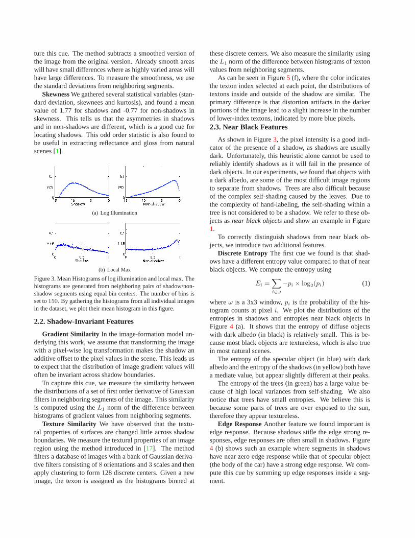
Intensity Difference Since shadows are expected to berelatively dark, we gather statistics (Figure3 (a)) about theintensity of image segments. In neighboring pixels, wemeasure the intensity difference using their absolute differ-ence. In neighboring segments, we measure the differenceusingL1 norm between the histograms of intensity values.We also augment the feature vector with the averaged inten-sity value and the standard deviation.

Local Max In a local patch, shadows have values thatare very low in intensity; therefore, the local max value isexpected to be small. On the contrary, non-shadows oftenhave values with high intensities and the local max value isexpected to be large (Figure3 (b)). We capture this cue bya local max completed at 3 pixel intervals.

SmoothnessShadows are often a smoothed version oftheir neighbors. This is because shadows tend to suppresslocal variations on the underlining surfaces. We use themethod proposed by Forsyth and Fleck in [9, 18] to cap-

ture this cue. The method subtracts a smoothed version ofthe image from the original version. Already smooth areaswill have small differences where as highly varied areas willhave large differences. To measure the smoothness, we usethe standard deviations from neighboring segments.

SkewnessWe gathered several statistical variables (stan-dard deviation, skewnees and kurtosis), and found a meanvalue of 1.77 for shadows and -0.77 for non-shadows inskewness. This tells us that the asymmetries in shadowsand in non-shadows are different, which is a good cue forlocating shadows. This odd order statistic is also found tobe useful in extracting reflectance and gloss from naturalscenes [1].

(a) Log Illumination

(b) Local Max

Figure 3. Mean Histograms of log illumination and local max. Thehistograms are generated from neighboring pairs of shadow/non-shadow segments using equal bin centers. The number of bins isset to150. By gathering the histograms from all individual imagesin the dataset, we plot their mean histogram in this figure.

2.2. Shadow-Invariant Features

Gradient Similarity In the image-formation model un-derlying this work, we assume that transforming the imagewith a pixel-wise log transformation makes the shadow anadditive offset to the pixel values in the scene. This leads usto expect that the distribution of image gradient values willoften be invariant across shadow boundaries.

To capture this cue, we measure the similarity betweenthe distributions of a set of first order derivative of Gaussianfilters in neighboring segments of the image. This similarityis computed using theL1 norm of the difference betweenhistograms of gradient values from neighboring segments.

Texture Similarity We have observed that the textu-ral properties of surfaces are changed little across shadowboundaries. We measure the textural properties of an imageregion using the method introduced in [17]. The methodfilters a database of images with a bank of Gaussian deriva-tive filters consisting of8 orientations and3 scales and thenapply clustering to form 128 discrete centers. Given a newimage, the texon is assigned as the histograms binned at

these discrete centers. We also measure the similarity usingtheL1 norm of the difference between histograms of textonvalues from neighboring segments.

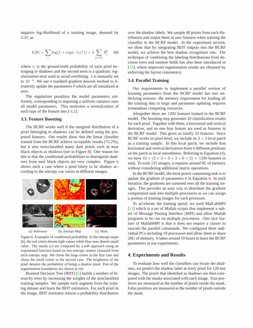
As can be seen in Figure5 (f), where the color indicatesthe texton index selected at each point, the distributions oftextons inside and outside of the shadow are similar. Theprimary difference is that distortion artifacts in the darkerportions of the image lead to a slight increase in the numberof lower-index textons, indicated by more blue pixels.2.3. Near Black Features

As shown in Figure3, the pixel intensity is a good indi-cator of the presence of a shadow, as shadows are usuallydark. Unfortunately, this heuristic alone cannot be used toreliably identify shadows as it will fail in the presence ofdark objects. In our experiments, we found that objects witha dark albedo, are some of the most difficult image regionsto separate from shadows. Trees are also difficult becauseof the complex self-shading caused by the leaves. Due tothe complexity of hand-labeling, the self-shading within atree is not considered to be a shadow. We refer to these ob-jects asnear black objectsand show an example in Figure1.

To correctly distinguish shadows from near black ob-jects, we introduce two additional features.

Discrete Entropy The first cue we found is that shad-ows have a different entropy value compared to that of nearblack objects. We compute the entropy using

Ei =∑

i∈ω

−pi × log2(pi) (1)

whereω is a 3x3 window,pi is the probability of the his-togram counts at pixeli. We plot the distributions of theentropies in shadows and entropies near black objects inFigure 4 (a). It shows that the entropy of diffuse objectswith dark albedo (in black) is relatively small. This is be-cause most black objects are textureless, which is also truein most natural scenes.

The entropy of the specular object (in blue) with darkalbedo and the entropy of the shadows (in yellow) both havea mediate value, but appear slightly different at their peaks.

The entropy of the trees (in green) has a large value be-cause of high local variances from self-shading. We alsonotice that trees have small entropies. We believe this isbecause some parts of trees are over exposed to the sun,therefore they appear textureless.

Edge ResponseAnother feature we found important isedge response. Because shadows stifle the edge strong re-sponses, edge responses are often small in shadows. Figure4 (b) shows such an example where segments in shadowshave near zero edge response while that of specular object(the body of the car) have a strong edge response. We com-pute this cue by summing up edge responses inside a seg-ment.

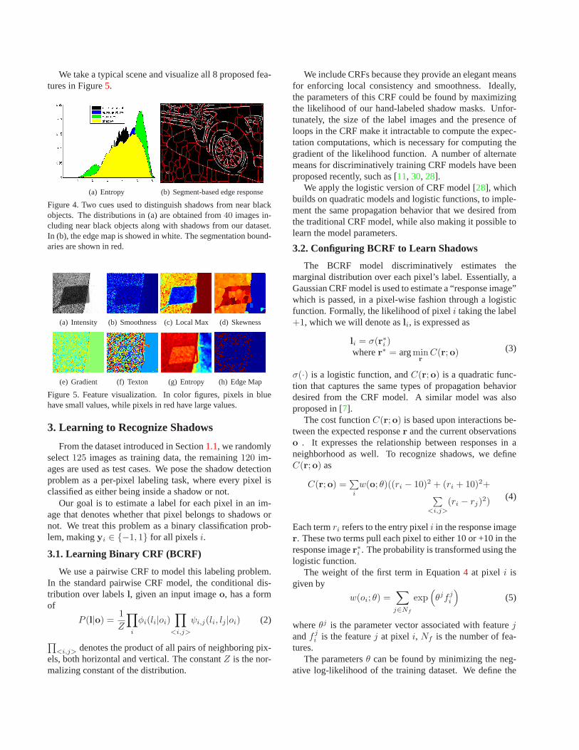
We take a typical scene and visualize all 8 proposed fea-tures in Figure5.

(a) Entropy (b) Segment-based edge response

Figure 4. Two cues used to distinguish shadows from near blackobjects. The distributions in (a) are obtained from40 images in-cluding near black objects along with shadows from our dataset.In (b), the edge map is showed in white. The segmentation bound-aries are shown in red.

(a) Intensity (b) Smoothness (c) Local Max (d) Skewness

(e) Gradient (f) Texton (g) Entropy (h) Edge Map

Figure 5. Feature visualization. In color figures, pixels in bluehave small values, while pixels in red have large values.

3. Learning to Recognize Shadows

From the dataset introduced in Section1.1, we randomlyselect125 images as training data, the remaining120 im-ages are used as test cases. We pose the shadow detectionproblem as a per-pixel labeling task, where every pixel isclassified as either being inside a shadow or not.

Our goal is to estimate a label for each pixel in an im-age that denotes whether that pixel belongs to shadows ornot. We treat this problem as a binary classification prob-lem, makingyi ∈ {−1, 1} for all pixelsi.

3.1. Learning Binary CRF (BCRF)

We use a pairwise CRF to model this labeling problem.In the standard pairwise CRF model, the conditional dis-tribution over labelsl, given an input imageo, has a formof

P (l|o) =1

Z

∏

i

φi(li|oi)∏

<i,j>

ψi,j(li, lj |oi) (2)

∏

<i,j> denotes the product of all pairs of neighboring pix-els, both horizontal and vertical. The constantZ is the nor-malizing constant of the distribution.

We include CRFs because they provide an elegant meansfor enforcing local consistency and smoothness. Ideally,the parameters of this CRF could be found by maximizingthe likelihood of our hand-labeled shadow masks. Unfor-tunately, the size of the label images and the presence ofloops in the CRF make it intractable to compute the expec-tation computations, which is necessary for computing thegradient of the likelihood function. A number of alternatemeans for discriminatively training CRF models have beenproposed recently, such as [11, 30, 28].

We apply the logistic version of CRF model [28], whichbuilds on quadratic models and logistic functions, to imple-ment the same propagation behavior that we desired fromthe traditional CRF model, while also making it possible tolearn the model parameters.

3.2. Configuring BCRF to Learn Shadows

The BCRF model discriminatively estimates themarginal distribution over each pixel’s label. Essentially, aGaussian CRF model is used to estimate a “response image”which is passed, in a pixel-wise fashion through a logisticfunction. Formally, the likelihood of pixeli taking the label+1, which we will denote asli, is expressed as

li = σ(r∗i )wherer∗ = argmin

r

C(r;o) (3)

σ(·) is a logistic function, andC(r;o) is a quadratic func-tion that captures the same types of propagation behaviordesired from the CRF model. A similar model was alsoproposed in [7].

The cost functionC(r;o) is based upon interactions be-tween the expected responser and the current observationso . It expresses the relationship between responses in aneighborhood as well. To recognize shadows, we defineC(r;o) as

C(r;o) =∑

i

w(o; θ)((ri − 10)2 + (ri + 10)2+∑

<i,j>

(ri − rj)2)

(4)

Each termri refers to the entry pixeli in the response imager. These two terms pull each pixel to either 10 or +10 in theresponse imager∗i . The probability is transformed using thelogistic function.

The weight of the first term in Equation4 at pixel i isgiven by

w(oi; θ) =∑

j∈Nf

exp(

θjfji

)

(5)

whereθj is the parameter vector associated with featurej

andf ji is the featurej at pixel i, Nf is the number of fea-

tures.The parametersθ can be found by minimizing the neg-

ative log-likelihood of the training dataset. We define the

negative log-likelihood of a training image, denoted byL(θ) as

L(θ) =∑

i

log(1 + exp(−tir∗

i )) + λ∑

j∈Nf

θ2j (6)

whereti is the ground-truth probability of each pixel be-longing to shadows and the second term is a quadratic reg-ularization term used to avoid overfitting.λ is manually setto 10−4. We use a standard gradient descent method to it-eratively update the parametersθ which are all initialized atzero.

The regularizer penalizes the model parameters uni-formly, corresponding to imposing a uniform variance ontoall model parameters. This motivates a normalization ofeach type of the feature into [-1,1].

3.3. Feature Boosting

The BCRF works well if the marginal distribution of apixel belonging to shadows can be defined using the pro-posed features. Our results show that the linear classifiertrained from the BCRF achieve acceptable results (75.2%),but it also missclassified many dark pixels such as nearblack objects as shadows (see in Figure8). One reason forthis is that the conditional probabilities to distinguish shad-ows from near black objects are very complex. Figure6shows such a case where a pixel likely to be shadow ac-cording to the entropy cue varies in different images.

(a) Reference (b) Entropy Map (c) Mask

Figure 6. Examples of conditional probability. In the entropy maps(b), the red colors denote high values while blue ones denote smallvalue. The masks (c) are computed by a soft approach using anexponential function based on two entropy centers clustered fromeach entropy map. We chose the large center in the first case andchose the small center in the second case. The brightness of thepixel denotes the probability of being a shadow pixel. Part of thesegmentation boundaries are shown in red.

Boosted Decision Tree (BDT) [5] builds a number of hi-erarchy trees by increasing the weights of the misclassifiedtraining samples. We sample each segment from the train-ing dataset and learn the BDT estimators. For each pixel inthe image, BDT estimator returns a probability distribution

over the shadow labels. We sample 40 points from each dis-tribution and output them as new features when training theclassifier in the BCRF model. In the experiment section,we show that by integrating BDT outputs into the BCRFmodel, we achieve the best shadow recognition rate. Thetechnique of combining the labeling distributions from de-cision trees and random fields has also been introduced in[33], where improved segmentation results are obtained byenforcing the layout consistency.

3.4. Parallel Training

Our requirements to implement a parallel version oflearning parameters from the BCRF model has two un-derlying reasons: the memory requirement for loading allthe training data is large and parameter updating requirestremendous computing resources.

Altogether there are1290 features trained in the BCRFmodel. The boosting step generates40 classification resultsfor each pixel. Together with them, a horizontal and verticalderivative, and an one bias feature are used as features inthe BCRF model. This gives us totally43 features. SinceBCRF works in pixel-level, we include its3× 3 local patchas a training sample. In this local patch, we include firsthorizontal and vertical derivatives from6 different positionson the patch as local smoothness. Referring to Equation (4),we have43 × (3 × 3 + 3 × 3 + 6 × 2) = 1290 features intotal. To train125 images, it requires around 9G of memorywithout considering additional matrix operations.

In the BCRF model, the most power consuming task is toupdate the gradient of parametersθ in Equation6. In eachiteration, the gradients are summed over all the training im-ages. This provides an easy way to distribute the gradientcomputation task into multiple processors as we can assigna portion of training images for each processor.

To accelerate the training speed, we used MatLabMPI[13] which is a set of Matlab scripts that implement a sub-set of Message Passing Interface (MPI) and allow Matlabprograms to be run on multiple processors. One nice fea-ture of MatlabMPI is that it does not require a cluster toexecute the parallel commands. We configured three indi-vidual PCs including 10 processors and allow them to share20G of memory. It takes around 10 hours to learn the BCRFparameters in our experiments.

4. Experiments and Results

To evaluate how well the classifiers can locate the shad-ows, we predict the shadow label at every pixel for 120 testimages. The pixels that identified as shadows are then com-pared with the masks associated with each image. True pos-itives are measured as the number of pixels inside the mask.False positives are measured as the number of pixels outsidethe mask.

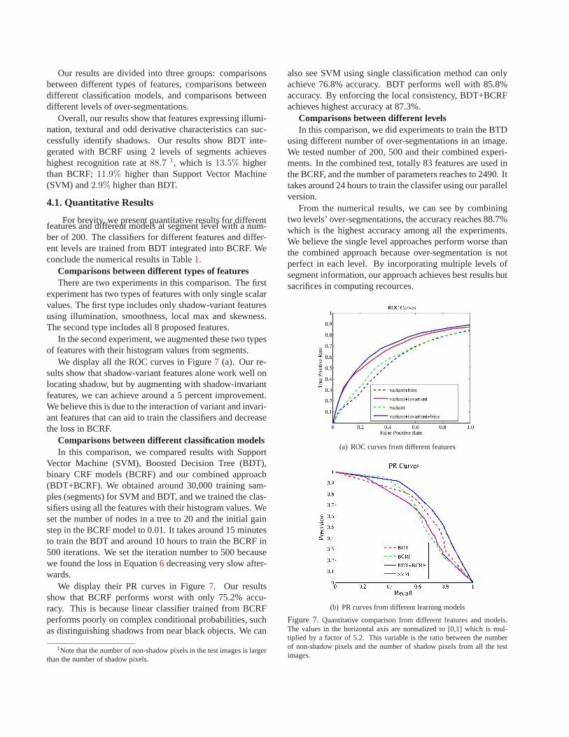
Our results are divided into three groups: comparisonsbetween different types of features, comparisons betweendifferent classification models, and comparisons betweendifferent levels of over-segmentations.

Overall, our results show that features expressing illumi-nation, textural and odd derivative characteristics can suc-cessfully identify shadows. Our results show BDT inte-gerated with BCRF using 2 levels of segments achieveshighest recognition rate at88.7 1, which is 13.5% higherthan BCRF;11.9% higher than Support Vector Machine(SVM) and2.9% higher than BDT.

4.1. Quantitative Results

For brevity, we present quantitative results for differentfeatures and different models at segment level with a num-ber of 200. The classifiers for different features and differ-ent levels are trained from BDT integrated into BCRF. Weconclude the numerical results in Table1.

Comparisons between different types of featuresThere are two experiments in this comparison. The first

experiment has two types of features with only single scalarvalues. The first type includes only shadow-variant featuresusing illumination, smoothness, local max and skewness.The second type includes all 8 proposed features.

In the second experiment, we augmented these two typesof features with their histogram values from segments.

We display all the ROC curves in Figure7 (a). Our re-sults show that shadow-variant features alone work well onlocating shadow, but by augmenting with shadow-invariantfeatures, we can achieve around a 5 percent improvement.We believe this is due to the interaction of variant and invari-ant features that can aid to train the classifiers and decreasethe loss in BCRF.

Comparisons between different classification modelsIn this comparison, we compared results with Support

Vector Machine (SVM), Boosted Decision Tree (BDT),binary CRF models (BCRF) and our combined approach(BDT+BCRF). We obtained around 30,000 training sam-ples (segments) for SVM and BDT, and we trained the clas-sifiers using all the features with their histogram values. Weset the number of nodes in a tree to 20 and the initial gainstep in the BCRF model to 0.01. It takes around 15 minutesto train the BDT and around 10 hours to train the BCRF in500 iterations. We set the iteration number to 500 becausewe found the loss in Equation6 decreasing very slow after-wards.

We display their PR curves in Figure7. Our resultsshow that BCRF performs worst with only 75.2% accu-racy. This is because linear classifier trained from BCRFperforms poorly on complex conditional probabilities, suchas distinguishing shadows from near black objects. We can

1Note that the number of non-shadow pixels in the test images is largerthan the number of shadow pixels.

also see SVM using single classification method can onlyachieve 76.8% accuracy. BDT performs well with 85.8%accuracy. By enforcing the local consistency, BDT+BCRFachieves highest accuracy at 87.3%.

Comparisons between different levelsIn this comparison, we did experiments to train the BTD

using different number of over-segmentations in an image.We tested number of 200, 500 and their combined experi-ments. In the combined test, totally 83 features are used inthe BCRF, and the number of parameters reaches to 2490. Ittakes around 24 hours to train the classifer using our parallelversion.

From the numerical results, we can see by combiningtwo levels’ over-segmentations, the accuracy reaches 88.7%which is the highest accuracy among all the experiments.We believe the single level approaches perform worse thanthe combined approach because over-segmentation is notperfect in each level. By incorporating multiple levels ofsegment information, our approach achieves best results butsacrifices in computing recources.

(a) ROC curves from different features

(b) PR curves from different learning models

Figure 7.Quantitative comparison from different features and models.The values in the horizontal axis are normalized to [0,1] which is mul-tiplied by a factor of 5.2. This variable is the ratio betweenthe numberof non-shadow pixels and the number of shadow pixels from all the testimages.

Table 1. Numerical Comparison of different methodsMethod Accuracy

Features

Discrepancy 82.3%Discrepancy+Bins 80.7%

Discrepancy+Consistency 86.7%Discrepancy+Consistency+Bins 87.3%

Models

SVM 76.8%Boosted Decision Tree 85.8%

Logistic CRFs 75.2%BDT+LRF 87.3%

Levels200 Segments 87.3%500 Segments 86.3%

Combine 200 and 500 Segments 88.7%

4.2. Qualitative Results

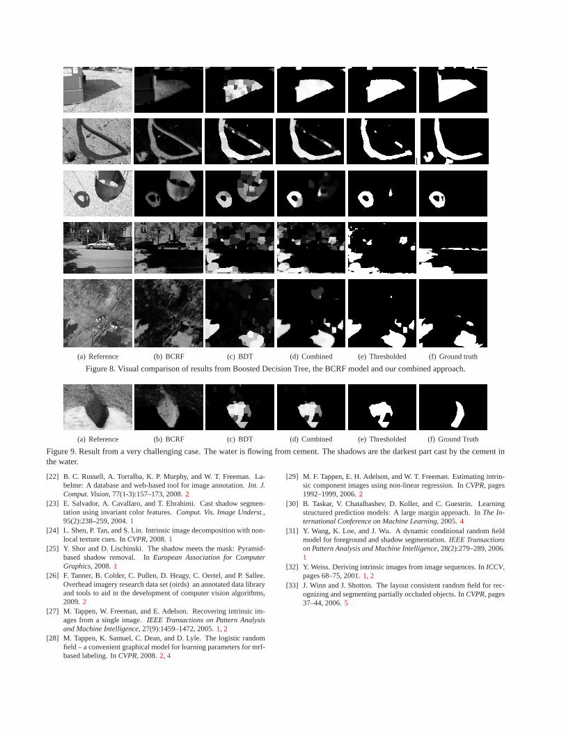
We present part of the qualitative results from our testresults in Figure8. We set the threshold to 0.5 when obtain-ing the binary estimates. For brevity, we only present theresults using combined levels of segments.

The first case shows a simple scene with shadows castedon the grass. The probability map from BDT is unsurpris-ingly inconsistent because BDT treats each segment indi-vidually. The result from CRF model alone is neither per-fect as we can see some misclassified pixels on the grassand near object boundaries.

The second and third cases show two examples of objectswith dark albedo. We can see the probabilities of such ob-jects being shadows from BCRF alone are falsely as high asreal shadows. Results from BDT are also not acceptable asthresholding the correct shadows from all the probabilitiesis very difficult.

The fourth and fifth cases show two complex examples.We can see BCRF model can not distinguish shadows fromtrees. BDT does good job on separating shadows from trees,but the labeling is inconsistent.

From all these test examples, we can see our combinedapproach performs better, in terms of both accuracy andconsistency, than either of BDT or BCRF model alone.

We show an example from very challenging case in Fig-ure9. The shadows in this scene are casted on water, whichis a transparent media and also appears black. The opti-cal properties of the shadows in the water are not capturedwell using our proposed features, therefore, both BDT andBCRF perorms poorly.

5. Conclusions

We have proposed a learning-based approach to recog-nize shadows from monochromatic natural images. Usingthe cues presented in this paper, our method can success-fully identify shadows in real-world data where color is un-available. We found that while single-pixel classificationstrategies work well, a Boosted Decision Tree integratedinto a CRF-based model achieves the best results.

6. Acknowledgement

This work was supported by a grant from the NGA NURIprogram(HM1582-08-1-0021),We would also like to thankDr. Jian Sun for helpful discussions..

References[1] E. Adelson. Image statistics and surface perception. InHuman Vision

and Electronic Imaging XIII, Proceedings of the SPIE, Volume 6806,pages 680602–680609, 2008.3

[2] E. Arbel and H. Hel-Ord. Texture-preserving shadow removal incolor images containing curved surfaces. InCVPR, 2007.1

[3] V. Ar evalo, J. Gonzalez, and G. Ambrosio. Shadow detectionin colour high-resolution satellite images.Int. J. Remote Sens.,29(7):1945–1963, 2008.1

[4] M. Bell and W. Freeman. Learning local evidence for shading andreflection. InICCV, 2001.1, 2

[5] M. Collins, R. E. Schapire, and Y. Singer. Logistic regression, ad-aboost and bregman distances. InMACHINE LEARNING, pages158–169, 2000.5

[6] R. Dror, A. Willsky, and E. Adelson. Statistical characterization ofreal-world illumination.Journal of Vision, 4(9):821–837, 2004.2

[7] M. A. T. Figueiredo. Bayesian image segmentation using gaussianfield priors. InEnergy Minimization Methods in Computer Visionand Pattern Recognition, 2005.4

[8] G. Finlayson, S. Hordley, C. Lu, and M. Drew. On the removalofshadows from images.IEEE Transactions on Pattern Analysis andMachine Intelligence, 28(1):59–68, 2006.1

[9] A. D. Forsyth and M. Fleck. Identifying nude pictures. InIEEEWorkshop on the Applications of Computer Vision, pages 103–108,1996.2

[10] A. K. Frederick, C. Beauce, and L. Hunter. Colour visionbringsclarity to shadows.Perception, 33(8):907–914, 2004.1

[11] T. Joachims, T. Finley, and C.-N. Yu. Cutting-plane training of struc-tural svms.Machine Learning, 76(1), 2009.4

[12] A. Joshi and N. Papanikolopoulos. Learning to detect moving shad-ows in dynamic environments.IEEE Transactions on Pattern Analy-sis and Machine Intelligence, 30(11):2055–2063, 2008.1

[13] J. Kepner. Matlabmpi.J. Parallel Distrib. Comput., 64(8):997–1005,2004.5

[14] D. Kersten, D. Knill, P. Mamassian, and I. Bulthoff. Illusory motionfrom shadows.Nature, 379:31, 1996.1

[15] M. D. Levine and J. Bhattacharyya. Removing shadows.PatternRecogn. Lett., 26(3):251–265, 2005.1

[16] N. Martel-Brisson and A. Zaccarin. Learning and removing castshadows through a multidistribution approach.IEEE Transactions onPattern Analysis and Machine Intelligence, 29(7):1133–1146, 2007.1

[17] D. R. Martin, C. C. Fowlkes, and J. Malik. Learning to detect natu-ral image boundaries using local brightness, color, and texture cues.IEEE Transactions on Pattern Analysis and Machine Intelligence,26(5):530–549, 2004.2, 3

[18] K. McHenry, J. Ponce, and D. Forsyth. Finding glass. InCVPR,pages 973–979, Washington, DC, USA, 2005. IEEE Computer Soci-ety. 2

[19] S. Nadimi and B. Bhanu. Physical models for moving shadow andobject detection in video.IEEE Transactions on Pattern Analysis andMachine Intelligence, 26(8):1079–1087, 2004.1

[20] A. Prati, I. Mikic, M. Trivedi, and R. Cucchiara. Detecting movingshadows: Algorithms and evaluation.IEEE Transactions on PatternAnalysis and Machine Intelligence, 25(7):918–923, 2003.2

[21] J. Rittscher, J. Kato, S. Joga, and A. Blake. A probabilistic back-ground model for tracking. InECCV, pages 336–350, 2000.1

l

(a) Reference (b) BCRF (c) BDT (d) Combined (e) Thresholded (f) Ground truth

Figure 8. Visual comparison of results from Boosted Decision Tree, theBCRF model and our combined approach.

(a) Reference (b) BCRF (c) BDT (d) Combined (e) Thresholded (f) Ground Truth

Figure 9. Result from a very challenging case. The water is flowing fromcement. The shadows are the darkest part cast by the cement inthe water.

[22] B. C. Russell, A. Torralba, K. P. Murphy, and W. T. Freeman. La-belme: A database and web-based tool for image annotation.Int. J.Comput. Vision, 77(1-3):157–173, 2008.2

[23] E. Salvador, A. Cavallaro, and T. Ebrahimi. Cast shadow segmen-tation using invariant color features.Comput. Vis. Image Underst.,95(2):238–259, 2004.1

[24] L. Shen, P. Tan, and S. Lin. Intrinsic image decompositionwith non-local texture cues. InCVPR, 2008.1

[25] Y. Shor and D. Lischinski. The shadow meets the mask: Pyramid-based shadow removal. InEuropean Association for ComputerGraphics, 2008.1

[26] F. Tanner, B. Colder, C. Pullen, D. Heagy, C. Oertel, andP. Sallee.Overhead imagery research data set (oirds) an annotated datalibraryand tools to aid in the development of computer vision algorithms,2009.2

[27] M. Tappen, W. Freeman, and E. Adelson. Recovering intrinsic im-ages from a single image.IEEE Transactions on Pattern Analysisand Machine Intelligence, 27(9):1459–1472, 2005.1, 2

[28] M. Tappen, K. Samuel, C. Dean, and D. Lyle. The logistic randomfield – a convenient graphical model for learning parameters for mrf-based labeling. InCVPR, 2008.2, 4

[29] M. F. Tappen, E. H. Adelson, and W. T. Freeman. Estimating intrin-sic component images using non-linear regression. InCVPR, pages1992–1999, 2006.2

[30] B. Taskar, V. Chatalbashev, D. Koller, and C. Guestrin.Learningstructured prediction models: A large margin approach. InThe In-ternational Conference on Machine Learning, 2005.4

[31] Y. Wang, K. Loe, and J. Wu. A dynamic conditional random fieldmodel for foreground and shadow segmentation.IEEE Transactionson Pattern Analysis and Machine Intelligence, 28(2):279–289, 2006.1

[32] Y. Weiss. Deriving intrinsic images from image sequences. In ICCV,pages 68–75, 2001.1, 2

[33] J. Winn and J. Shotton. The layout consistent random field for rec-ognizing and segmenting partially occluded objects. InCVPR, pages37–44, 2006.5