Learning to Reason with Extracted Information
82
Learning to Reason with Extracted Information William W. Cohen Carnegie Mellon University joint work with: William Wang, Kathryn Rivard Mazaitis, Stephen Muggleton, Tom Mitchell, Ni Lao, Richard Wang, Frank Lin, Ni Lao, Estevam Hruschka, Jr., Burr Settles, Partha Talukdar, Derry Wijaya, Edith Law, Justin Betteridge, Jayant Krishnamurthy, Bryan Kisiel, Andrew Carlson, Weam Abu Zaki , Bhavana Dalvi, Malcolm Greaves, Lise Getoor, Jay Pujara, Hui Miao, …
-
Upload
calvin-fischer -
Category
Documents
-
view
50 -
download
0
description
Learning to Reason with Extracted Information. William W. Cohen Carnegie Mellon University joint work with: William Wang, Kathryn Rivard Mazaitis , Stephen Muggleton, Tom Mitchell, Ni Lao, - PowerPoint PPT Presentation
Transcript of Learning to Reason with Extracted Information

Learning to Reason with Extracted Information
William W. CohenCarnegie Mellon University
joint work with:
William Wang, Kathryn Rivard Mazaitis, Stephen Muggleton, Tom Mitchell, Ni Lao,
Richard Wang, Frank Lin, Ni Lao, Estevam Hruschka, Jr., Burr Settles, Partha Talukdar, Derry Wijaya, Edith Law, Justin Betteridge, Jayant Krishnamurthy, Bryan Kisiel, Andrew
Carlson, Weam Abu Zaki , Bhavana Dalvi, Malcolm Greaves, Lise Getoor, Jay Pujara, Hui Miao, …
Outline
• Background: information extraction and NELL• Key ideas in NELL
– Coupled learning– Multi-view, multi-strategy learning
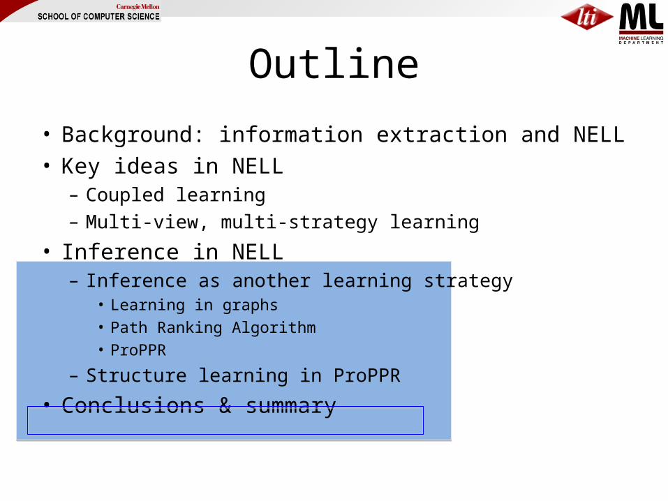
• Inference in NELL– Inference as another learning strategy
• Learning in graphs • Path Ranking Algorithm• ProPPR
– Structure learning in ProPPR
• Conclusions & summary

Never Ending Language Learning (NELL)
• NELL is a broad-coverage IE system– Simultaneously learning hundreds of concepts and relations
(person, celebrity, emotion, aquiredBy, locatedIn, capitalCityOf, ..)
– Starting point: containment/disjointness relations between concepts, types for relations, and O(10) examples per concept/relation, and large web corpus
– Running continuously for over four years– Has learned tens of millions of “beliefs”

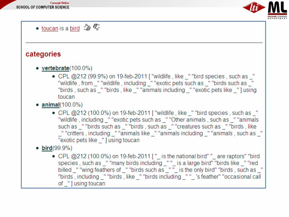
NELL Screenshots

More examples of what NELL knows

NP1 NP2
Krzyzewski coaches the Blue Devils.
athleteteam
coachesTeam(c,t)
person
coach
sport
playsForTeam(a,t)
NP
Krzyzewski coaches the Blue Devils.
coach(NP)
hard (underconstrained)semi-supervised learning
problem
much easier (more constrained)semi-supervised learning problem
teamPlaysSport(t,s)
playsSport(a,s)
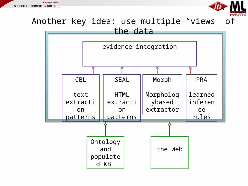
One Key: Coupled Semi-Supervised Learning
1. Easier to learn many interrelated tasks than one isolated task2. Also easier to learn using many different types of information
Ontology and
populated KB
the Web
CBL
text extraction patterns
SEAL
HTML extraction patterns
evidence integration
PRA
learned inference
rules
Morph
Morphologybased
extractor
Another key idea: use multiple “views” of the data

Outline
• Background: information extraction and NELL• Key ideas in NELL
– Coupled learning– Multi-view, multi-strategy learning
• Inference in NELL– Inference as another learning strategy
• Learning in graphs • Path Ranking Algorithm• ProPPR
– Structure learning in ProPPR
• Conclusions & summary

Motivations
• Short-term, practical: – Extend the knowledge base with additional
probabilistically-inferred facts– Understand noise, errors and regularities: e.g., is
“competes with” transitive?
• Long-term, fundamental:– From an AI perspective, inference is what you do with a
knowledge base– People do reason, so intelligent systems must reason:
• when you’re working with a user, you can’t wait for them to say something that they’ve inferred to be true
Summary of this section
• Background: where we’re coming from• ProPPR: the first-order extension of our past work• Parameter learning in ProPPR
– small-scale– medium-large scale
• Structure learning for ProPPR– small-scale– medium-scale …

Background

Learning about graph similarity:past work
• Personalized PageRank aka Random Walk with Restart: basically PageRank where surfer always “teleports” to a start node x.– Query: Given type t* and node x, find y:T(y)=t* and y~x– Answer: ranked list of y’s similar-to x
• Einat Minkov’s thesis (2008): Learning parameterized variants of personalized PageRank for PIM and language tasks.
• Ni Lao’s thesis (2012): New, better learning methods– richer parameterization: one parameter per “path”– faster inference
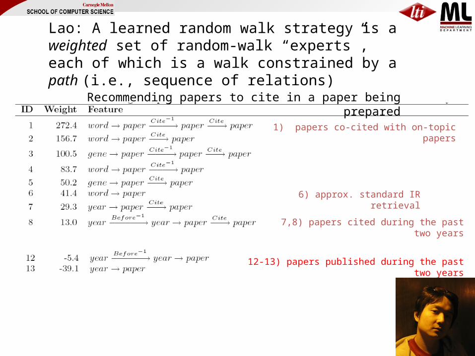
Lao: A learned random walk strategy is a weighted set of random-walk “experts”, each of which is a walk constrained by a path (i.e., sequence of relations)
6) approx. standard IR retrieval
1) papers co-cited with on-topic papers
7,8) papers cited during the past two years
12-13) papers published during the past two years
Recommending papers to cite in a paper being prepared
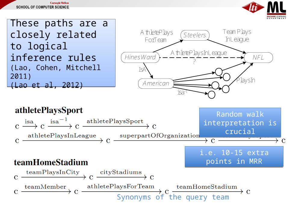
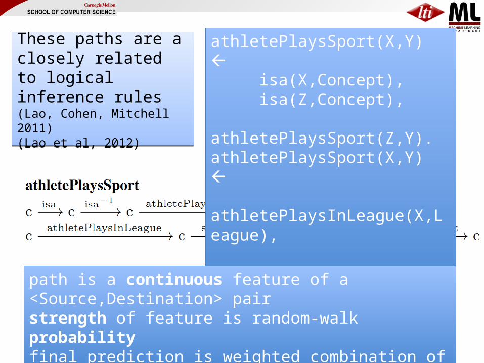
These paths are a closely related to logical inference rules(Lao, Cohen, Mitchell 2011)(Lao et al, 2012)
These paths are a closely related to logical inference rules(Lao, Cohen, Mitchell 2011)(Lao et al, 2012)
Synonyms of the query team
American
IsA
PlaysIn
AthletePlaysInLeagueHinesWard
SteelersAthletePlaysForTeam
NFL
TeamPlaysInLeague
?
isa-1
Random walk interpretation is crucial
Random walk interpretation is crucial
i.e. 10-15 extra points in MRRi.e. 10-15 extra points in MRR
These paths are a closely related to logical inference rules(Lao, Cohen, Mitchell 2011)(Lao et al, 2012)
These paths are a closely related to logical inference rules(Lao, Cohen, Mitchell 2011)(Lao et al, 2012)
Synonyms of the query team
athletePlaysSport(X,Y) isa(X,Concept), isa(Z,Concept), athletePlaysSport(Z,Y).athletePlaysSport(X,Y) athletePlaysInLeague(X,League), superPartOfOrg(League,Team), teamPlaysSport(Team,Y).
athletePlaysSport(X,Y) isa(X,Concept), isa(Z,Concept), athletePlaysSport(Z,Y).athletePlaysSport(X,Y) athletePlaysInLeague(X,League), superPartOfOrg(League,Team), teamPlaysSport(Team,Y).
path is a continuous feature of a <Source,Destination> pairstrength of feature is random-walk probabilityfinal prediction is weighted combination of these
path is a continuous feature of a <Source,Destination> pairstrength of feature is random-walk probabilityfinal prediction is weighted combination of these

Ontology and
populated KB
the Web
CBL
text extraction patterns
SEAL
HTML extraction patterns
evidence integration
PRA
learned inference
rules
Morph
Morphologybased
extractor
PRA is now part of NELLPRA is now part of NELL
On beyond path-ranking….

athletePlaySportViaRule(Athlete,Sport) onTeamViaKB(Athlete,Team), teamPlaysSportViaKB(Team,Sport)
teamPlaysSportViaRule(Team,Sport) memberOfViaKB(Team,Conference), hasMemberViaKB(Conference,Team2),playsViaKB(Team2,Sport).
teamPlaysSportViaRule(Team,Sport) onTeamViaKB(Athlete,Team), athletePlaysSportViaKB(Athlete,Sport)
A limitation of PRA• Paths are learned separately for each relation
type, and one learned rule can’t call another• So, PRA can learn this….

A limitation• Paths are learned separately for each relation
type, and one learned rule can’t call another• But PRA can not learn this…..
athletePlaySport(Athlete,Sport) onTeam(Athlete,Team), teamPlaysSport(Team,Sport)
athletePlaySport(Athlete,Sport) athletePlaySportViaKB(Athlete,Sport)
teamPlaysSport(Team,Sport) memberOf(Team,Conference), hasMember(Conference,Team2),plays(Team2,Sport).
teamPlaysSport(Team,Sport) onTeam(Athlete,Team), athletePlaysSport(Athlete,Sport)
teamPlaysSport(Team,Sport) teamPlaysSportViaKB(Team,Sport)
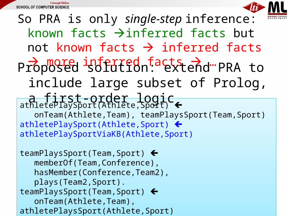
So PRA is only single-step inference: known facts inferred facts but not known facts inferred facts more inferred facts …
athletePlaySport(Athlete,Sport) onTeam(Athlete,Team), teamPlaysSport(Team,Sport)
athletePlaySport(Athlete,Sport) athletePlaySportViaKB(Athlete,Sport)
teamPlaysSport(Team,Sport) memberOf(Team,Conference), hasMember(Conference,Team2),plays(Team2,Sport).
teamPlaysSport(Team,Sport) onTeam(Athlete,Team), athletePlaysSport(Athlete,Sport)
teamPlaysSport(Team,Sport) teamPlaysSportViaKB(Team,Sport)
Proposed solution: extend PRA to include large subset of Prolog, a first-order logic
Programming with Personalized PageRank (ProPPR)
William Wang Kathryn Rivard Mazaitis

Sample ProPPR program….
Horn rules features of rules(generated on-the-fly)
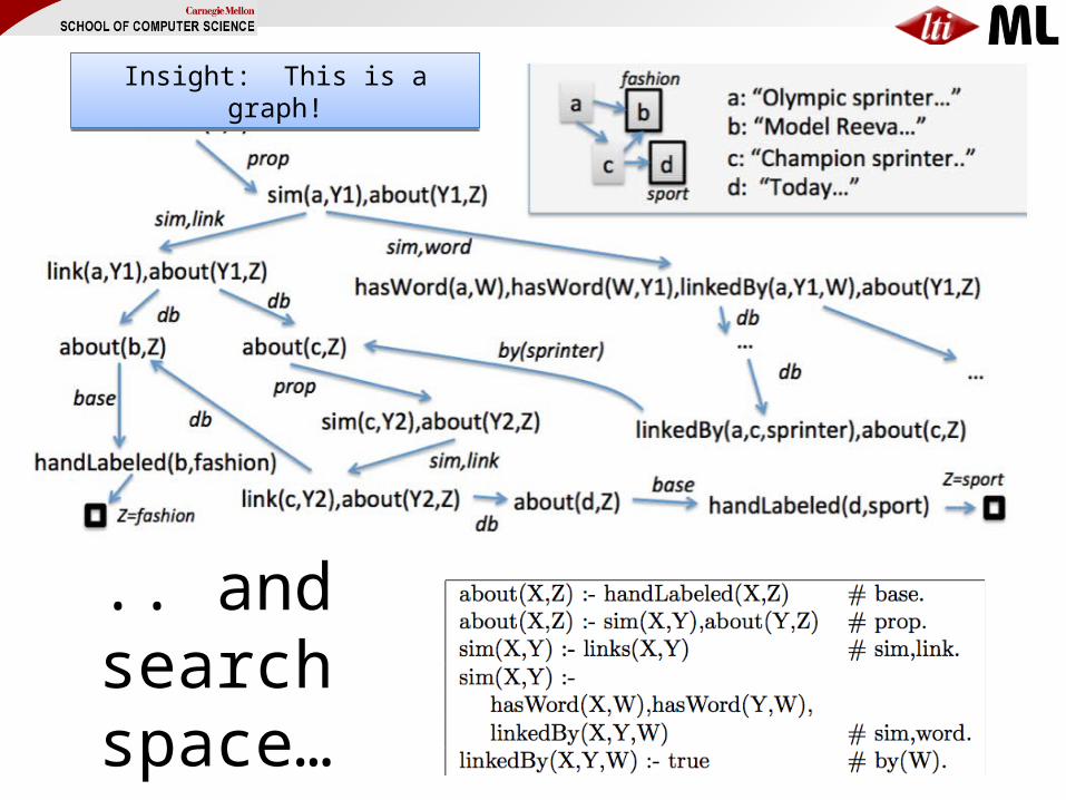
.. and search space…
Insight: This is a graph!Insight: This is a graph!
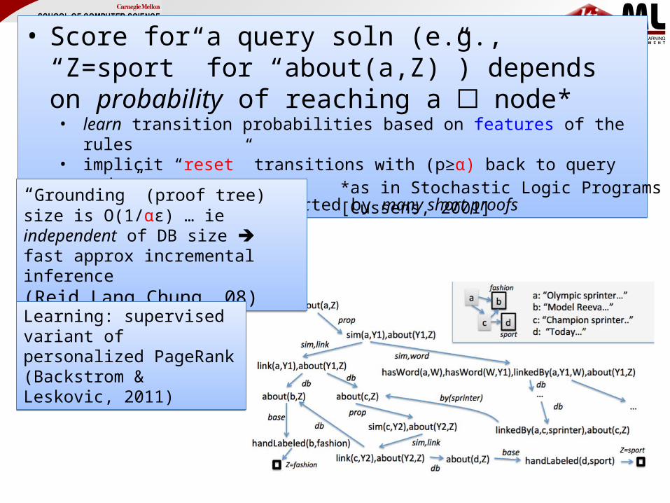
• Score for a query soln (e.g., “Z=sport” for “about(a,Z)”) depends on probability of reaching a ☐ node*• learn transition probabilities based on features of the rules• implicit “reset” transitions with (p≥α) back to query node
• Looking for answers supported by many short proofs
• Score for a query soln (e.g., “Z=sport” for “about(a,Z)”) depends on probability of reaching a ☐ node*• learn transition probabilities based on features of the rules• implicit “reset” transitions with (p≥α) back to query node
• Looking for answers supported by many short proofs
“Grounding” (proof tree) size is O(1/αε) … ie independent of DB size fast approx incremental inference (Reid,Lang,Chung, 08)
“Grounding” (proof tree) size is O(1/αε) … ie independent of DB size fast approx incremental inference (Reid,Lang,Chung, 08)
Learning: supervised variant of personalized PageRank (Backstrom & Leskovic, 2011)
Learning: supervised variant of personalized PageRank (Backstrom & Leskovic, 2011)
*as in Stochastic Logic Programs[Cussens, 2001]

Programming with Personalized PageRank (ProPPR)
• Advantages:– Can attach arbitrary features to a clause– Minimal syntactic restrictions: can allow
recursion, multiple predicates, function symbols (!), ….
– Grounding cost -- conversion to the zero-th order learning problem -- does not depend on the number of known facts in the approximate proof case.

Inference Time: Citation Matchingvs Alchemy
“Grounding”cost is independent of DB size“Grounding”cost is independent of DB size
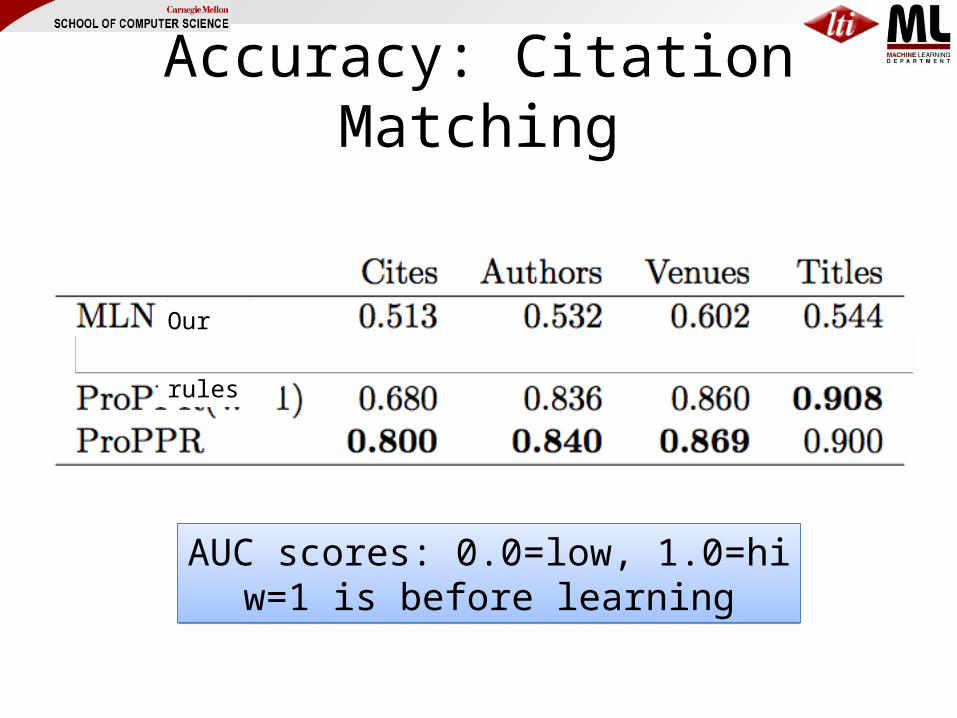
Accuracy: Citation Matching
AUC scores: 0.0=low, 1.0=hiw=1 is before learning
AUC scores: 0.0=low, 1.0=hiw=1 is before learning
UW rules
Our rules
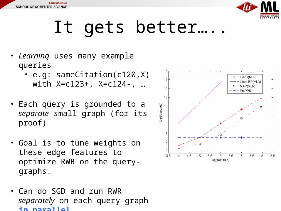
It gets better…..• Learning uses many example queries
• e.g: sameCitation(c120,X) with X=c123+, X=c124-, …
• Each query is grounded to a separate small graph (for its proof)
• Goal is to tune weights on these edge features to optimize RWR on the query-graphs.
• Can do SGD and run RWR separately on each query-graph in parallel
• Graphs do share edge features, so there’s some synchronization needed

Learning can be parallelized by splitting on the separate “groundings” of each queryLearning can be parallelized by splitting on the separate “groundings” of each query
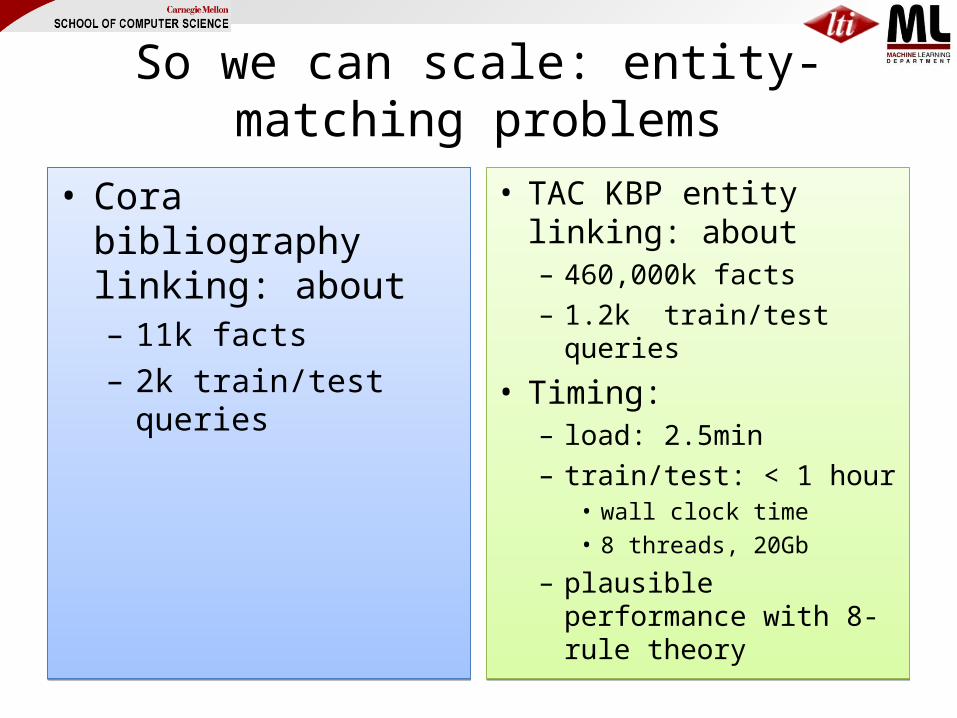
So we can scale: entity-matching problems
• Cora bibliography linking: about– 11k facts– 2k train/test queries
• Cora bibliography linking: about– 11k facts– 2k train/test queries
• TAC KBP entity linking: about– 460,000k facts– 1.2k train/test queries
• Timing:– load: 2.5min– train/test: < 1 hour
• wall clock time• 8 threads, 20Gb
– plausible performance with 8-rule theory
• TAC KBP entity linking: about– 460,000k facts– 1.2k train/test queries
• Timing:– load: 2.5min– train/test: < 1 hour
• wall clock time• 8 threads, 20Gb
– plausible performance with 8-rule theory
Using ProPPR to learn inference rules over NELL’s KB
See also William Wang’s poster here at NLU-2014
See also William Wang’s poster here at NLU-2014
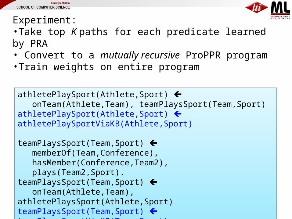
Experiment:•Take top K paths for each predicate learned by PRA• Convert to a mutually recursive ProPPR program•Train weights on entire program
athletePlaySport(Athlete,Sport) onTeam(Athlete,Team), teamPlaysSport(Team,Sport)
athletePlaySport(Athlete,Sport) athletePlaySportViaKB(Athlete,Sport)
teamPlaysSport(Team,Sport) memberOf(Team,Conference), hasMember(Conference,Team2),plays(Team2,Sport).
teamPlaysSport(Team,Sport) onTeam(Athlete,Team), athletePlaysSport(Athlete,Sport)
teamPlaysSport(Team,Sport) teamPlaysSportViaKB(Team,Sport)
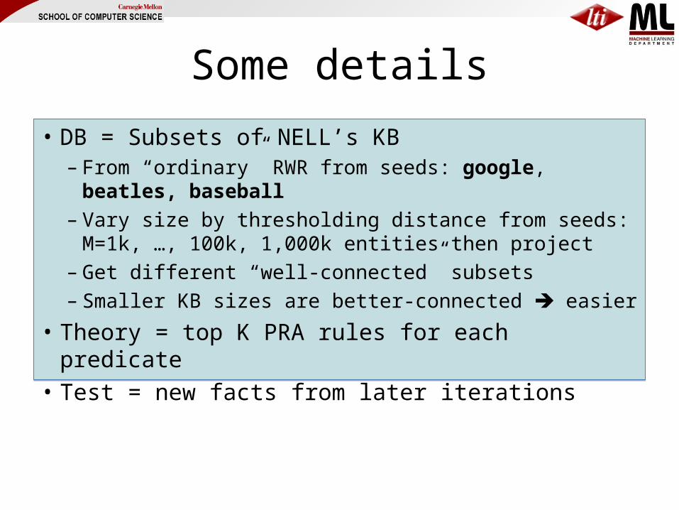
Some details
• DB = Subsets of NELL’s KB • Theory = top K PRA rules for each predicate• Test = new facts from later iterations
Some details
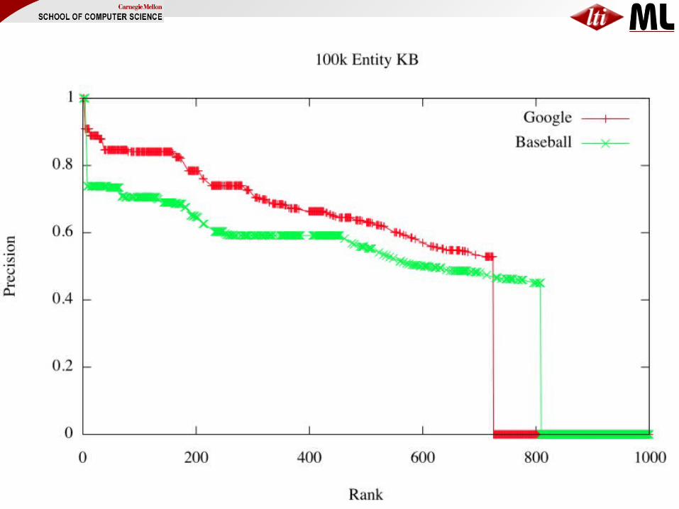
• DB = Subsets of NELL’s KB – From “ordinary” RWR from seeds: google,
beatles, baseball– Vary size by thresholding distance from seeds:
M=1k, …, 100k, 1,000k entities then project– Get different “well-connected” subsets– Smaller KB sizes are better-connected easier
• Theory = top K PRA rules for each predicate• Test = new facts from later iterations

Some details
• DB = Subsets of NELL’s KB • Theory = top K PRA rules for each predicate
– For PRA rule p(X,Y) :- q(Y,Z),r(Z,Y)• PRA recursive: q, r can invoke other rules AND
p(X,Y) can also be proved via KB lookup via a “base case rule”
• PRA non-recursive: q, r must be KB lookup• KB only: only the “base case” rules
• Test = new facts from later iterations

Some details
• DB = Subsets of NELL’s KB • Theory = top K PRA rules for each predicate• Test = new facts from later iterations
– Negative examples from ontology constraints

Results: AUC on test datavarying KB size
* KBs overlap a lot at 1M entities

Results: AUC on test datavarying theory size
100k (rec)
1M(rec)
top 1 ~ 430-540 ~ 550
top 2 ~ 620-770 ~ 800
top 3 ~800-1000 ~1000

Results: training time in sec

vs Alchemy/MLNs on 1k KB subset

Results: training time in sec
inference time as a function of KB size: varying KB from 10k to 50k entities
Outline
• Background: information extraction and NELL• Key ideas in NELL
– Coupled learning– Multi-view, multi-strategy learning
• Inference in NELL– Inference as another learning strategy
• Learning in graphs • Path Ranking Algorithm• ProPPR
– Structure learning in ProPPR
• Conclusions & summary
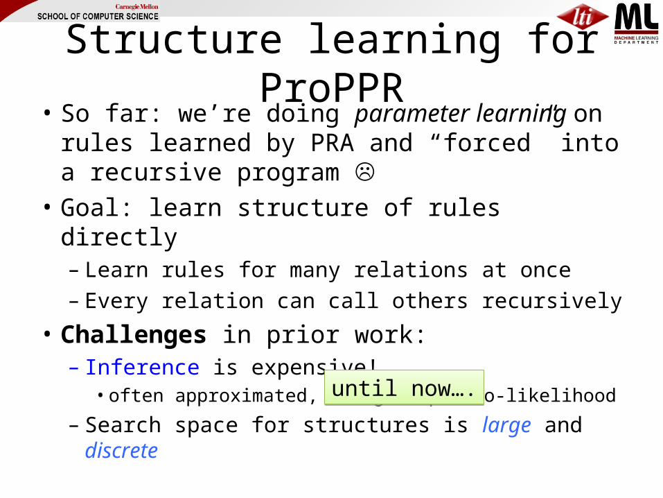
Structure learning for ProPPR• So far: we’re doing parameter learning on
rules learned by PRA and “forced” into a recursive program
• Goal: learn structure of rules directly– Learn rules for many relations at once– Every relation can call others recursively
• Challenges in prior work:– Inference is expensive!
• often approximated, using ~= pseudo-likelihood
– Search space for structures is large and discrete
until now….until now….

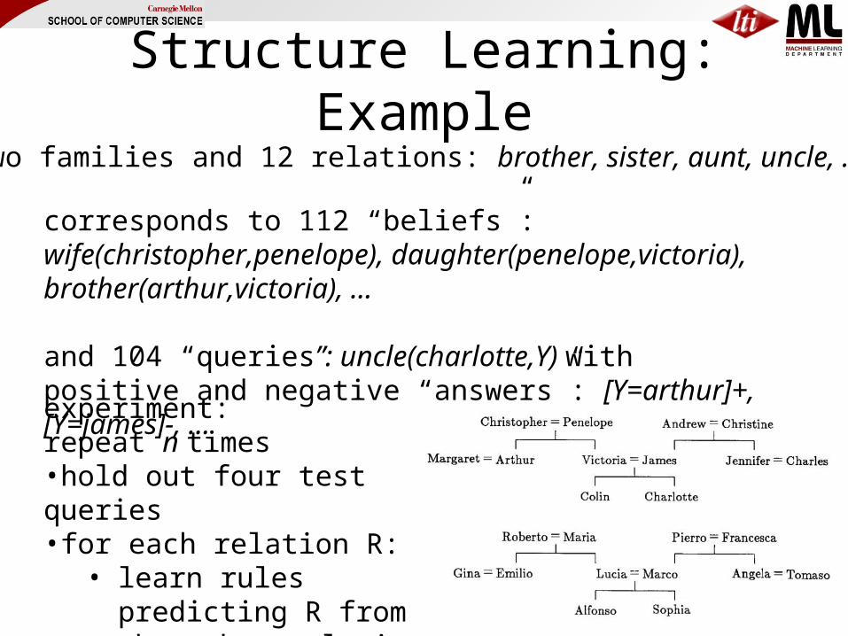
Structure Learning: Exampletwo families and 12 relations: brother, sister, aunt, uncle, …
Structure Learning: Exampletwo families and 12 relations: brother, sister, aunt, uncle, …
corresponds to 112 “beliefs”: wife(christopher,penelope), daughter(penelope,victoria), brother(arthur,victoria), …
and 104 “queries”: uncle(charlotte,Y) with positive and negative “answers”: [Y=arthur]+, [Y=james]-, …
experiment: repeat n times•hold out four test queries•for each relation R:
• learn rules predicting R from the other relations
•test

Structure Learning: Exampletwo families and 12 relations: brother, sister, aunt, uncle, …
Result: •7/8 tests correct (Hinton 1986)•78/80 tests correct (Quinlan 1990, FOIL)
•but…..
Result: •7/8 tests correct (Hinton 1986)•78/80 tests correct (Quinlan 1990, FOIL)
•but…..
experiment: repeat n times•hold out four test queries•for each relation R:
• learn rules predicting R from the other relations
•test
Structure Learning: Exampletwo families and 12 relations: brother, sister, aunt, uncle, …
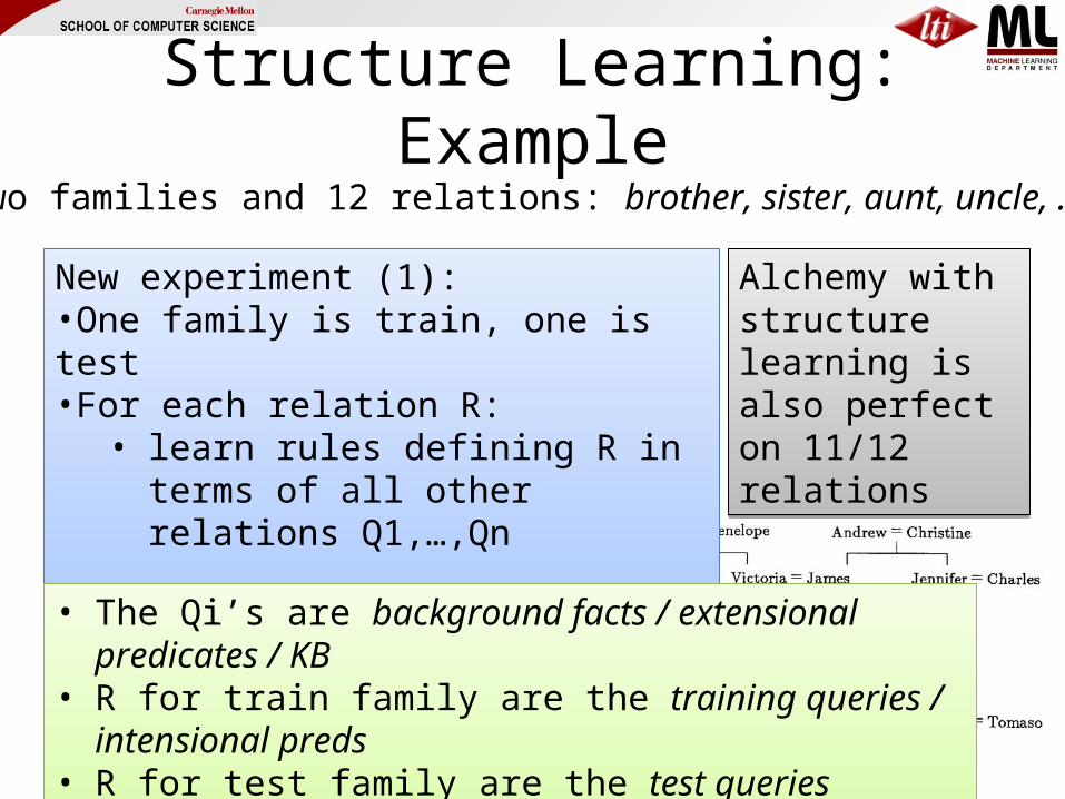
New experiment (1):•One family is train, one is test•For each relation R:
• learn rules defining R in terms of all other relations Q1,…,Qn
•Result: 100% accuracy! (with FOIL, c 1990)
New experiment (1):•One family is train, one is test•For each relation R:
• learn rules defining R in terms of all other relations Q1,…,Qn
•Result: 100% accuracy! (with FOIL, c 1990)
• The Qi’s are background facts / extensional predicates / KB• R for train family are the training queries / intensional preds• R for test family are the test queries
• The Qi’s are background facts / extensional predicates / KB• R for train family are the training queries / intensional preds• R for test family are the test queries
Alchemy with structure learning is also perfect on 11/12 relations
Alchemy with structure learning is also perfect on 11/12 relations
Structure Learning: Exampletwo families and 12 relations: brother, sister, aunt, uncle, …
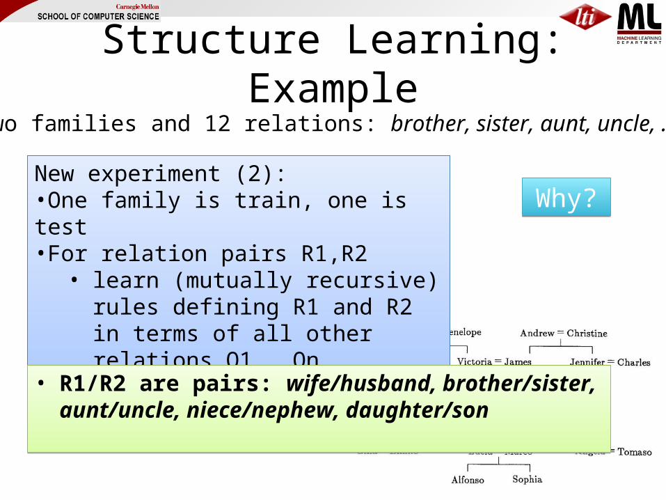
New experiment (2):•One family is train, one is test•For relation pairs R1,R2
• learn (mutually recursive) rules defining R1 and R2 in terms of all other relations Q1,…,Qn
•Result: 0% accuracy! (with FOIL, c 1990)
New experiment (2):•One family is train, one is test•For relation pairs R1,R2
• learn (mutually recursive) rules defining R1 and R2 in terms of all other relations Q1,…,Qn
•Result: 0% accuracy! (with FOIL, c 1990)
• R1/R2 are pairs: wife/husband, brother/sister, aunt/uncle, niece/nephew, daughter/son
• R1/R2 are pairs: wife/husband, brother/sister, aunt/uncle, niece/nephew, daughter/son
Why?Why?
Structure Learning: Exampletwo families and 12 relations: brother, sister, aunt, uncle, …
New experiment (2):•One family is train, one is test•For relation pairs R1,R2
• learn (mutually recursive) rules defining R1 and R2 in terms of all other relations Q1,…,Qn
•Result: 0% accuracy! (with FOIL, c 1990)
New experiment (2):•One family is train, one is test•For relation pairs R1,R2
• learn (mutually recursive) rules defining R1 and R2 in terms of all other relations Q1,…,Qn
•Result: 0% accuracy! (with FOIL, c 1990)
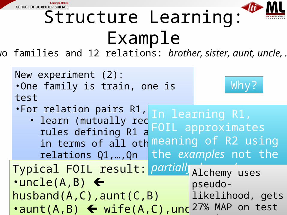
Typical FOIL result:•uncle(A,B) husband(A,C),aunt(C,B)•aunt(A,B) wife(A,C),uncle(C,B)
Typical FOIL result:•uncle(A,B) husband(A,C),aunt(C,B)•aunt(A,B) wife(A,C),uncle(C,B)
Why?Why?
In learning R1, FOIL approximates meaning of R2 using the examples not the partially learned program
In learning R1, FOIL approximates meaning of R2 using the examples not the partially learned program
Alchemy uses pseudo-likelihood, gets 27% MAP on test queries
Alchemy uses pseudo-likelihood, gets 27% MAP on test queries
Structure Learning: Exampletwo families and 12 relations: brother, sister, aunt, uncle, …
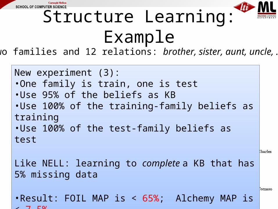
New experiment (3):•One family is train, one is test•Use 95% of the beliefs as KB•Use 100% of the training-family beliefs as training•Use 100% of the test-family beliefs as test
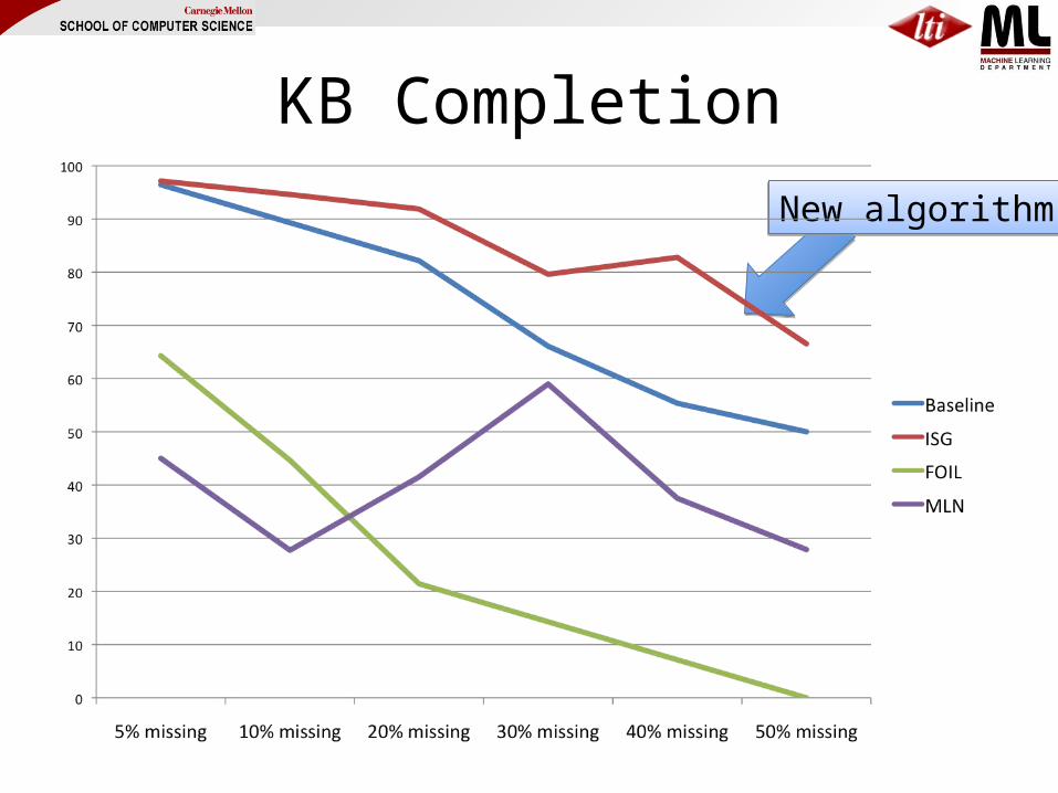
Like NELL: learning to complete a KB that has 5% missing data
•Result: FOIL MAP is < 65%; Alchemy MAP is < 7.5%•Baseline MAP using incomplete KB: 96.4%
New experiment (3):•One family is train, one is test•Use 95% of the beliefs as KB•Use 100% of the training-family beliefs as training•Use 100% of the test-family beliefs as test
Like NELL: learning to complete a KB that has 5% missing data
•Result: FOIL MAP is < 65%; Alchemy MAP is < 7.5%•Baseline MAP using incomplete KB: 96.4%

KB Completion
KB Completion
New algorithmNew algorithm

Structure learning for ProPPR• Goal: learn structure of rules
– Learn rules for many relations at once– Every relation can call others recursively
• Challenges in prior work:– Inference is expensive!
• often approximated, using ~= pseudo-likelihood
– Search space for structures is large and discrete
until now….until now….
reduce structure learning to parameter learning via the “Metagol trick” [Muggleton et al] reduce structure learning to parameter learning via the “Metagol trick” [Muggleton et al]

The “Metagol” Approach
• Start with an “abductive second order theory” that defines the space of structures.
• Introduce minimal set of assumptions needed to prove that the positive examples are covered.– Each assumption is about the existence of a rule in the
learned theory.• Metagol uses iterative deepening to search for minimal
assumptions (and hence theory) and learns a “hard” theory.
• Here’s how we translate this to ProPPR…
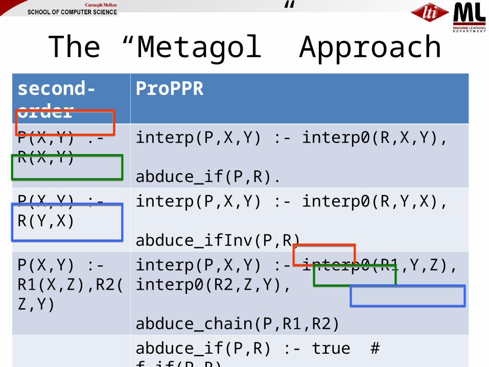
The “Metagol” Approachsecond-order ProPPR
P(X,Y) :- R(X,Y) interp(P,X,Y) :- interp0(R,X,Y), abduce_if(P,R).
P(X,Y) :- R(Y,X) interp(P,X,Y) :- interp0(R,Y,X), abduce_ifInv(P,R).
P(X,Y) :- R1(X,Z),R2(Z,Y)
interp(P,X,Y) :- interp0(R1,Y,Z), interp0(R2,Z,Y), abduce_chain(P,R1,R2)
abduce_if(P,R) :- true # f_if(P,R)abduce_ifInv(P,R) :- true # f_ifInv(P,R)abduce_chain(P,R1,R2) :- true # f_chain(P,R1,R2)
interp0(P,X,Y) :- kbContains(P,X,Y)
interp(uncle,joe,Y) interp0(R,Y,joe), abduce_ifInv(uncle,R)
kbContains(R,Y,joe), abduce_ifInv(uncle,R)
interp(uncle,joe,Y) interp0(R,Y,joe), abduce_ifInv(uncle,R)
kbContains(R,Y,joe), abduce_ifInv(uncle,R)
kbContains(nephew,sam,joe), abduce_ifInv(uncle,nephew)kbContains(nephew,sam,joe), abduce_ifInv(uncle,nephew)
interp(uncle,joe,sam)interp(uncle,joe,sam)
truetrue
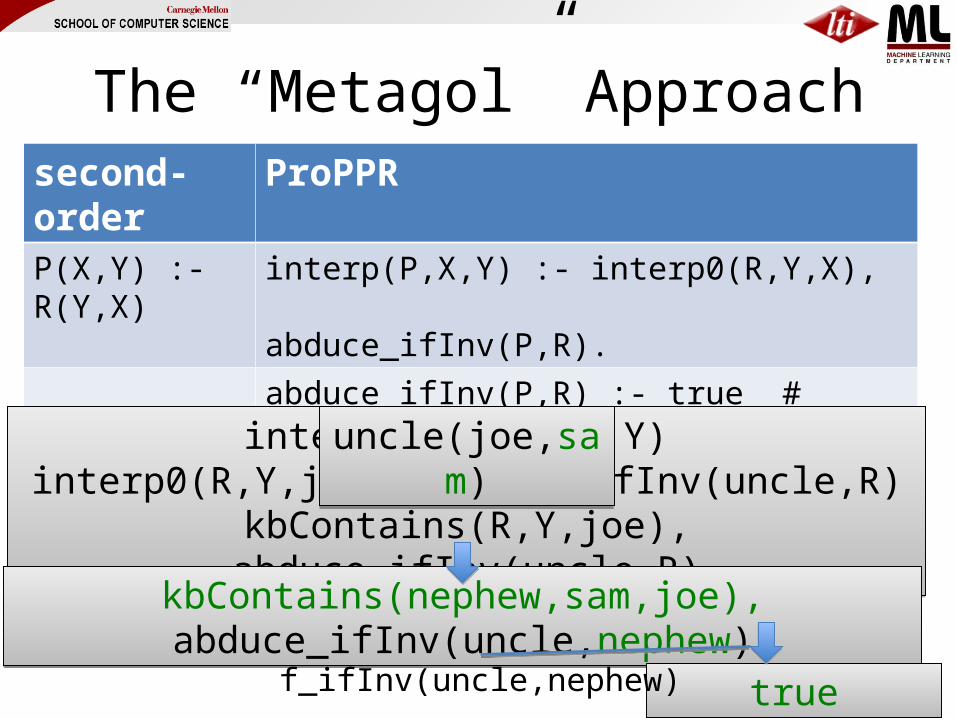
The “Metagol” Approachsecond-order ProPPRP(X,Y) :- R(Y,X) interp(P,X,Y) :- interp0(R,Y,X),
abduce_ifInv(P,R).abduce_ifInv(P,R) :- true # f_ifInv(P,R)
interp(uncle,joe,Y) interp0(R,Y,joe), abduce_ifInv(uncle,R)
kbContains(R,Y,joe), abduce_ifInv(uncle,R)
interp(uncle,joe,Y) interp0(R,Y,joe), abduce_ifInv(uncle,R)
kbContains(R,Y,joe), abduce_ifInv(uncle,R)
kbContains(nephew,sam,joe), abduce_ifInv(uncle,nephew)kbContains(nephew,sam,joe), abduce_ifInv(uncle,nephew)
uncle(joe,sam)uncle(joe,sam)
truetruef_ifInv(uncle,nephew)

The “Metagol” Approachsecond-order ProPPR
P(X,Y) :- R(X,Y) interp(P,X,Y) :- interp0(R,X,Y), abduce_if(P,R).
P(X,Y) :- R(Y,X) interp(P,X,Y) :- interp0(R,Y,X), abduce_ifInv(P,R).
P(X,Y) :- R1(X,Z),R2(Z,Y)
interp(P,X,Y) :- interp0(R1,Y,Z), interp0(R2,Z,Y), abduce_chain(P,R1,R2)
abduce_if(P,R) :- true # f_if(P,R)abduce_ifInv(P,R) :- true # f_ifInv(P,R)abduce_chain(P,R1,R2) :- true # f_chain(P,R1,R2)
interp0(P,X,Y) :- kbContains(P,X,Y)
Proof will follow a 2-step PRA-style path and then introduce a feature naming it.
Proof will follow a 2-step PRA-style path and then introduce a feature naming it.
Longer paths, etc: a few more second-order rules.Longer paths, etc: a few more second-order rules.

Iterated Structural Gradient: Idea
• Main idea:– Features (and parameters) in the second-order theory ~=
first-order rules– But, the second-order theory is much slower:
• Second-order: do a random walk (interpret a clause), and then accept (or more likely reject) it
• First-order: just use the clauses you need– So: interleave gradient steps in the second-order theory
with addition of the corresponding first-order rules for parameters with useful gradients
• But translate these rules into the second-order syntax….

Iterated Structural Gradient: Algorithm
• For t=1,…– Compute gradient of loss for the second-
order theory– See which features reduce loss: f_if(p,q),
f_ifInv(q,p), f_chain(p,q,r), ….– Add the corresponding rules to the
“second-order” theory: p(X,Y) :- q(X,Y), p(X,Y):-q(Y,X), p(X,Y):-q(Y,Z),r(Z,Y), ..

The “Metagol” Approach: Examplesecond-order ProPPR
P(X,Y) :- R(X,Y) interp(P,X,Y) :- interp0(R,X,Y), abduce_if(P,R).
P(X,Y) :- R(Y,X) interp(P,X,Y) :- interp0(R,Y,X), abduce_ifInv(P,R).
P(X,Y) :- R1(X,Z),R2(Z,Y)
interp(P,X,Y) :- interp0(R1,Y,Z), interp0(R2,Z,Y), abduce_chain(P,R1,R2)
abduce_if(P,R) :- true # f_if(P,R)abduce_ifInv(P,R) :- true # f_ifInv(P,R)abduce_chain(P,R1,R2) :- true # f_chain(P,R1,R2)
interp0(P,X,Y) :- kbContains(P,X,Y)interp0(uncle,X,Y) :- interp0(nephew,Y,X)
f_inv(uncle,nephew)f_inv(uncle,nephew)

Iterated Structural Gradient
• For t=1,…– Compute gradient of loss of the second-order theory– See which features reduce loss: f_if(p,q), f_ifInv(q,p),
f_chain(p,q,r), ….– Add the corresponding rules to the “second-order” theory– Repeat…until no more rules are added
• Discard second-order rules and re-learn parameter weights.
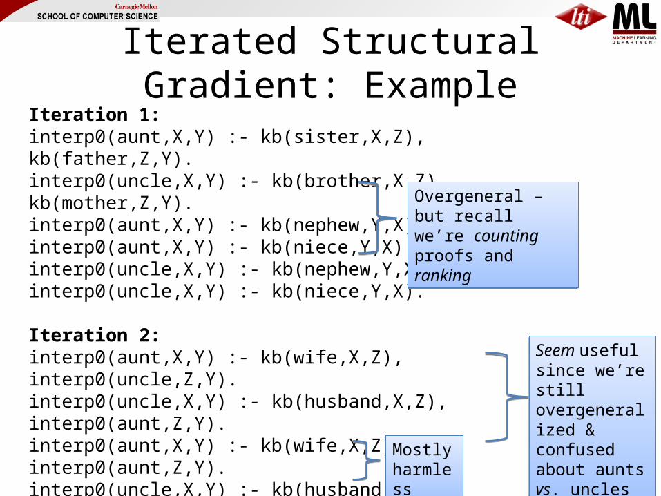
Iterated Structural Gradient: ExampleIteration 1:interp0(aunt,X,Y) :- kb(sister,X,Z), kb(father,Z,Y).interp0(uncle,X,Y) :- kb(brother,X,Z), kb(mother,Z,Y).interp0(aunt,X,Y) :- kb(nephew,Y,X).interp0(aunt,X,Y) :- kb(niece,Y,X).interp0(uncle,X,Y) :- kb(nephew,Y,X).interp0(uncle,X,Y) :- kb(niece,Y,X).
Iteration 2:interp0(aunt,X,Y) :- kb(wife,X,Z), interp0(uncle,Z,Y).interp0(uncle,X,Y) :- kb(husband,X,Z), interp0(aunt,Z,Y).interp0(aunt,X,Y) :- kb(wife,X,Z), interp0(aunt,Z,Y).interp0(uncle,X,Y) :- kb(husband,X,Z), interp0(uncle,Z,Y).interp0(aunt,X,Y) :- interp0(uncle,X,Y).interp0(uncle,X,Y) :- interp0(aunt,X,Y).interp0(aunt,X,Y) :- interp0(aunt,X,Y).interp0(uncle,X,Y) :- interp0(uncle,X,Y).
Overgeneral – but recall we’re counting proofs and ranking
Overgeneral – but recall we’re counting proofs and ranking
Seem useful since we’re still overgeneralized & confused about aunts vs. uncles
Seem useful since we’re still overgeneralized & confused about aunts vs. unclesMostly
harmlessMostly harmless
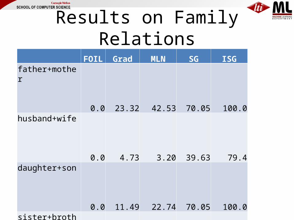
Results on Family RelationsFOIL Grad MLN SG ISG
father+mother 0.0 23.32 42.53 70.05 100.0husband+wife 0.0 4.73 3.20 39.63 79.4daughter+son 0.0 11.49 22.74 70.05 100.0sister+brother 0.0 3.29 10.37 62.18 78.85uncle+aunt 0.0 10.41 53.35 79.41 100.0niece+nephew 0.0 6.49 28.54 72.25 80.09average 0.0 9.96 26.79 65.60 89.70
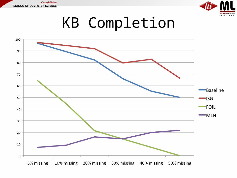
KB Completion

Summary of this section
• Background: where we’re coming from• ProPPR: the first-order extension of our past work• Parameter learning in ProPPR
– small-scale– medium-large scale
• Structure learning for ProPPR– small-scale– medium-scale …
Completing the NELL KB
• DB = Subsets of NELL’s KB– Subsets selected as before
• Theory – learned via ISG– Randomly-selected N beliefs used for training– Disjoint set of N beliefs used for test
• No negative information used!
– Rest used as background/KB
• We’re testing activity of completing a (noisy) KB: not (yet) the correctness of the beliefs

Outline
• Background: information extraction and NELL• Key ideas in NELL
– Coupled learning– Multi-view, multi-strategy learning
• Inference in NELL– Inference as another learning strategy
• Learning in graphs • Path Ranking Algorithm• ProPPR
– Structure learning in ProPPR
• Conclusions & summary

Summary
• What can you do with a large real-world KB?– Probabilistic inference: derive new facts from it, using plausible
inference rules– Structure learning: learn plausible inference rules from data
• Probabilistic inference is very challenging– … especially when you’re interested in scaling– Existing systems are restricted to inference over small KBs, highly
restricted logics, or both– Big problem: the grounding problem (translation to a non-first order
representation)– Structural learning is challenging2
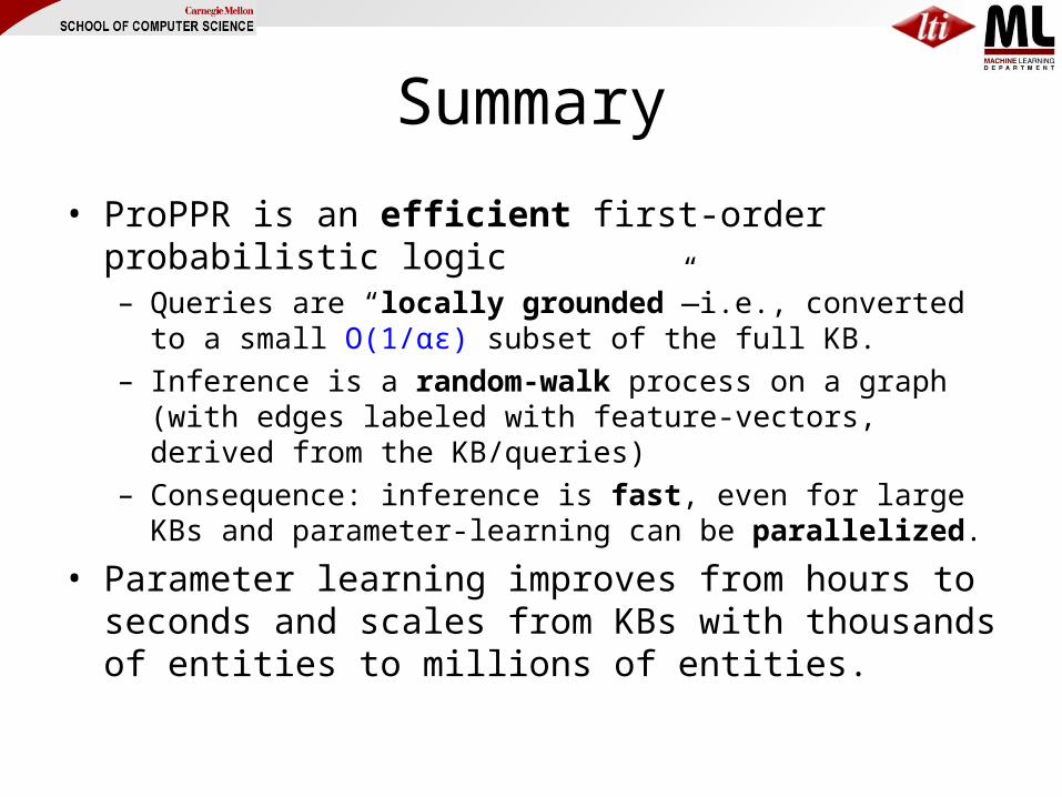
Summary
• ProPPR is an efficient first-order probabilistic logic– Queries are “locally grounded”—i.e., converted to a small O(1/αε)
subset of the full KB.– Inference is a random-walk process on a graph (with edges labeled
with feature-vectors, derived from the KB/queries)– Consequence: inference is fast, even for large KBs and parameter-
learning can be parallelized.
• Parameter learning improves from hours to seconds and scales from KBs with thousands of entities to millions of entities.
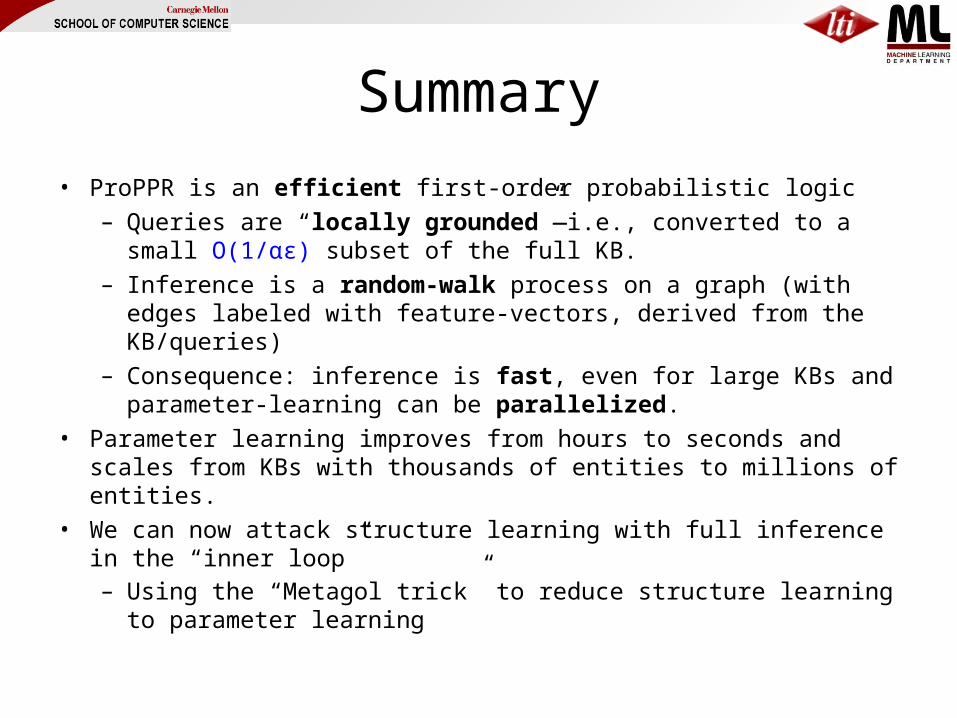
Summary• ProPPR is an efficient first-order probabilistic logic
– Queries are “locally grounded”—i.e., converted to a small O(1/αε) subset of the full KB.
– Inference is a random-walk process on a graph (with edges labeled with feature-vectors, derived from the KB/queries)
– Consequence: inference is fast, even for large KBs and parameter-learning can be parallelized.
• Parameter learning improves from hours to seconds and scales from KBs with thousands of entities to millions of entities.
• We can now attack structure learning with full inference in the “inner loop”– Using the “Metagol trick” to reduce structure learning to parameter
learning

Future Work on ProPPR
• Other joint-learning applications• More memory-efficient structures, integrating
external classifiers, etc• Constrained learning
– currently learning can push reset weights too low
• Learning better-integrated with proofs– currently learning uses power-iteration
computation for PPR, not approximation scheme used in theorem-proving

Thank You!

Backup Slides
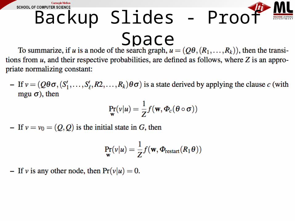
Backup Slides - Proof Space
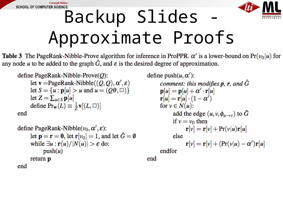
Backup Slides - Approximate Proofs

Backup Slides - Exact Proofs

Backup Slides - Loss

![Design and Development of a Personal Learning Environment ... · M. N. Ndongfack 3 Figure 1. Self-regulated learning process model. Extracted from [4]. 2.1. Personal Learning Environment](https://static.fdocuments.net/doc/165x107/5f3281b50c3fce580d12634d/design-and-development-of-a-personal-learning-environment-m-n-ndongfack-3.jpg)