Learning to Localize Sound Source in Visual Scenes

Arda Senocak1 Tae-Hyun Oh2 Junsik Kim1 Ming-Hsuan Yang3 In So Kweon1

Dept. EE, KAIST, South Korea1

MIT CSAIL, MA, USA2

Dept. EECS, University of California, Merced, CA, USA3

Abstract

Visual events are usually accompanied by sounds in our

daily lives. We pose the question: Can the machine learn

the correspondence between visual scene and the sound,

and localize the sound source only by observing sound and

visual scene pairs like human? In this paper, we propose a

novel unsupervised algorithm to address the problem of lo-

calizing the sound source in visual scenes. A two-stream

network structure which handles each modality, with at-

tention mechanism is developed for sound source localiza-

tion. Moreover, although our network is formulated within

the unsupervised learning framework, it can be extended

to a unified architecture with a simple modification for the

supervised and semi-supervised learning settings as well.

Meanwhile, a new sound source dataset is developed for

performance evaluation. Our empirical evaluation shows

that the unsupervised method eventually go through false

conclusion in some cases. We also show that even with a

few supervision, i.e., semi-supervised setup, false conclu-

sion is able to be corrected effectively.

1. Introduction

Visual events are typically coherent with sounds and they

are integrated. When we see that a car is moving, we hear

the engine sound at the same time. Sound carries rich infor-

mation regarding the spatial and temporal cues of the source

within a visual scene. As shown in the bottom example of

Figure 1, the engine sound suggests where the source may

be in the physical world [11]. This implies that sound is

not only complementary to the visual information, but also

correlated to visual events.

Humans observe tremendous number of combined

*Acknowledgment: We thank to Wei-Sheng Lai for helpful discus-

sions, and to the annotators. A. Senocak, J. Kim and I.S. Kweon were sup-

ported by Institute for Information & communications Technology Promo-

tion (IITP) grant funded by the Korea government (MSIT) (2017-0-01780).

The part of this work was done when T.-H. Oh was in KAIST, and he was

partly funded by HBKU QCRI at MIT. M.-H. Yang is supported in part by

NSF CAREER (No. 1149783).

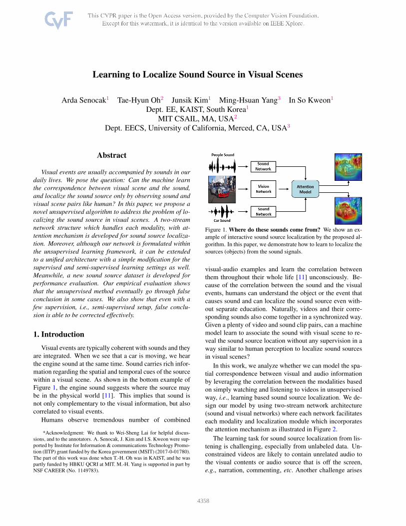
Figure 1. Where do these sounds come from? We show an ex-

ample of interactive sound source localization by the proposed al-

gorithm. In this paper, we demonstrate how to learn to localize the

sources (objects) from the sound signals.

visual-audio examples and learn the correlation between

them throughout their whole life [11] unconsciously. Be-

cause of the correlation between the sound and the visual

events, humans can understand the object or the event that

causes sound and can localize the sound source even with-

out separate education. Naturally, videos and their corre-

sponding sounds also come together in a synchronized way.

Given a plenty of video and sound clip pairs, can a machine

model learn to associate the sound with visual scene to re-

veal the sound source location without any supervision in a

way similar to human perception to localize sound sources

in visual scenes?

In this work, we analyze whether we can model the spa-

tial correspondence between visual and audio information

by leveraging the correlation between the modalities based

on simply watching and listening to videos in unsupervised

way, i.e., learning based sound source localization. We de-

sign our model by using two-stream network architecture

(sound and visual networks) where each network facilitates

each modality and localization module which incorporates

the attention mechanism as illustrated in Figure 2.

The learning task for sound source localization from lis-

tening is challenging, especially from unlabeled data. Un-

constrained videos are likely to contain unrelated audio to

the visual contents or audio source that is off the screen,

e.g., narration, commenting, etc. Another challenge arises

4358

�Localization

Module

FC

FC

FC

FC

⊗Supervised

Loss

Unsupervised

Loss

Avg. Pooling

Visual

CNN

Sound

CNN

(Semi-supervised case)

�����

Localization Response

: Layers : Features

�

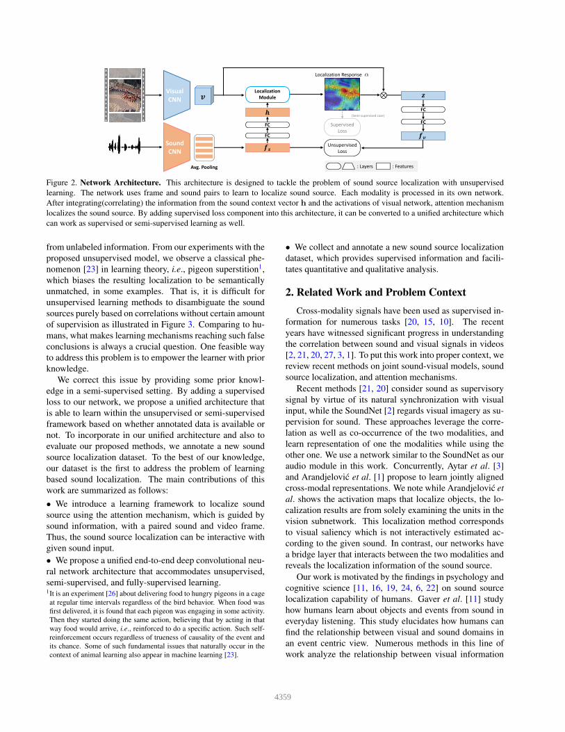
Figure 2. Network Architecture. This architecture is designed to tackle the problem of sound source localization with unsupervised

learning. The network uses frame and sound pairs to learn to localize sound source. Each modality is processed in its own network.

After integrating(correlating) the information from the sound context vector h and the activations of visual network, attention mechanism

localizes the sound source. By adding supervised loss component into this architecture, it can be converted to a unified architecture which

can work as supervised or semi-supervised learning as well.

from unlabeled information. From our experiments with the

proposed unsupervised model, we observe a classical phe-

nomenon [23] in learning theory, i.e., pigeon superstition1,

which biases the resulting localization to be semantically

unmatched, in some examples. That is, it is difficult for

unsupervised learning methods to disambiguate the sound

sources purely based on correlations without certain amount

of supervision as illustrated in Figure 3. Comparing to hu-

mans, what makes learning mechanisms reaching such false

conclusions is always a crucial question. One feasible way

to address this problem is to empower the learner with prior

knowledge.

We correct this issue by providing some prior knowl-

edge in a semi-supervised setting. By adding a supervised

loss to our network, we propose a unified architecture that

is able to learn within the unsupervised or semi-supervised

framework based on whether annotated data is available or

not. To incorporate in our unified architecture and also to

evaluate our proposed methods, we annotate a new sound

source localization dataset. To the best of our knowledge,

our dataset is the first to address the problem of learning

based sound localization. The main contributions of this

work are summarized as follows:

• We introduce a learning framework to localize sound

source using the attention mechanism, which is guided by

sound information, with a paired sound and video frame.

Thus, the sound source localization can be interactive with

given sound input.

• We propose a unified end-to-end deep convolutional neu-

ral network architecture that accommodates unsupervised,

semi-supervised, and fully-supervised learning.1It is an experiment [26] about delivering food to hungry pigeons in a cage

at regular time intervals regardless of the bird behavior. When food was

first delivered, it is found that each pigeon was engaging in some activity.

Then they started doing the same action, believing that by acting in that

way food would arrive, i.e., reinforced to do a specific action. Such self-

reinforcement occurs regardless of trueness of causality of the event and

its chance. Some of such fundamental issues that naturally occur in the

context of animal learning also appear in machine learning [23].

• We collect and annotate a new sound source localization

dataset, which provides supervised information and facili-

tates quantitative and qualitative analysis.

2. Related Work and Problem Context

Cross-modality signals have been used as supervised in-

formation for numerous tasks [20, 15, 10]. The recent

years have witnessed significant progress in understanding

the correlation between sound and visual signals in videos

[2, 21, 20, 27, 3, 1]. To put this work into proper context, we

review recent methods on joint sound-visual models, sound

source localization, and attention mechanisms.

Recent methods [21, 20] consider sound as supervisory

signal by virtue of its natural synchronization with visual

input, while the SoundNet [2] regards visual imagery as su-

pervision for sound. These approaches leverage the corre-

lation as well as co-occurrence of the two modalities, and

learn representation of one the modalities while using the

other one. We use a network similar to the SoundNet as our

audio module in this work. Concurrently, Aytar et al. [3]

and Arandjelovic et al. [1] propose to learn jointly aligned

cross-modal representations. We note while Arandjelovic et

al. shows the activation maps that localize objects, the lo-

calization results are from solely examining the units in the

vision subnetwork. This localization method corresponds

to visual saliency which is not interactively estimated ac-

cording to the given sound. In contrast, our networks have

a bridge layer that interacts between the two modalities and

reveals the localization information of the sound source.

Our work is motivated by the findings in psychology and

cognitive science [11, 16, 19, 24, 6, 22] on sound source

localization capability of humans. Gaver et al. [11] study

how humans learn about objects and events from sound in

everyday listening. This study elucidates how humans can

find the relationship between visual and sound domains in

an event centric view. Numerous methods in this line of

work analyze the relationship between visual information

4359

and sound localization. The findings demonstrate that vi-

sual information correlated to sound improves the efficiency

of search [16] and accuracy of localization [24]. Recent

research [19, 6, 22] extends the findings of human perfor-

mance on sound source localization against visual informa-

tion in 3D space. These studies evidently show that sound

source localization capability of humans is guided by visual

information, and two sources of information are closely cor-

related that humans can unconsciously learn the capability.

Prior to the recent advances of deep learning, compu-

tational methods for sound source localization rely on syn-

chrony [12] of low-level features of sounds and videos (e.g.,

raw waveform signals and intensity values respectively),

spatial sparsity prior of audio-visual events [18], low-

dimensionality [9], and hand-crafted motion cues as well

as segmentation [5, 14]. In contrast, the proposed network

is developed in an unsupervised manner by only watch-

ing and listening to videos without using any manually-

designed constraints such as motion. In addition, our semi-

supervised architecture accommodates minimal prior infor-

mation for better performance.

Acoustic based approach [30, 34] has been practically

used in surveillance and instrumentation engineering. It re-

quires specific devices, e.g., microphone arrays, to capture

phase differences of sound arrival. In this work, we learn

sound source localization in the visual domain without any

special devices but a microphone to capture sound.

Inspired by human attention mechanism [7], computa-

tional visual attention models [31, 33] have been developed.

However not only visual attentions but also the sound lo-

calization behavior in imagery resemble to the human at-

tention. In this work, we adopt the same attention mecha-

nism philosophy [31] to allow our networks to interact with

sound context and visual representation across spatial axes.

3. Proposed Algorithm

We design a neural network to address the problem of

vision based sound localization within the unsupervised

learning framework. In order to deal with cross-modality

signals from sounds and videos, we use a two-stream net-

work architecture. The network composes of three main

modules: sound network, visual network and attention

model as illustrated in Figure 2. We describe the main com-

ponents of each module in this section, and present more

network details as well as hyper-parameters in the supple-

mentary material.

3.1. Sound Network

For sound localization, it is important to capture the con-

cept of sound rather than catching low-level signal [11]. In

addition, sound signal is a 1-D signal with varying tempo-

ral length. We represent sound signals by using the con-

volutional module (conv), rectified linear unit (ReLu) and

pooling (pool), and stacking layers to encode high-level

concepts [32].

We use a 1-D deep convolutional architecture which is

invariant to input length as fully convolutional networks via

the use of average pooling over sliding windows. The pro-

posed sound network consists of 10 layers and takes raw

waveform as input. The first conv layers (up to conv8)

are similar to the SoundNet [2], but with 1000 filters fol-

lowed by average pooling across the temporal axis within a

sliding window (e.g., 20 seconds in this work).

Similar to the global average pooling which can handle

variable length inputs to be a fixed dimension vector [29],

the output activation of conv8 followed by average pooling

is always a single 1000-D vector by a sliding window. We

denote the sound representation after average pooling as fs.

To encode higher level concept of the sound signals, the

9-th and 10-th layers consist of ReLU followed by fully con-

nected (FC) layers. The output of the 10-th FC layer (FC10)

is 512-D, and is denoted as h. We use h to interact with

features from the visual network, and enforce h to resem-

ble visual concepts. Among these two features, we note fspreserves more sound concept while h captures correlation

information related to visual signals.

3.2. Visual Network

The visual network is composed of the image feature ex-

tractor and localization module. To extract features from

visual signals, we use an architecture similar to the VGG-

16 model [25] up to conv5 3 and feed a color video

frames of size H⇥W as input. We denote the activation of

conv5 3 as V2RH0⇥W 0⇥D, where H 0=bH16c, W 0=bW

16 cand D = 512. Each 512-D activation vector from conv5 3

contains local visual context information, and spatial infor-

mation is preserved in H 0⇥W 0 grid.

We make the activation V interact with the sound em-

bedding h for revealing sound source location information

in the grid, which is denoted as the localization module.

This localization module returns a confidence map of sound

source and a representative visual feature vector z corre-

sponding to location of source of the given input sound.

Once we obtain the visual feature z, it goes through two

{ReLu-FC} blocks to compute the visual embedding fv ,

which is the final output of the visual network.

3.3. Localization Network

Given extracted visual and sound concepts, the localiza-

tion networks generate the sound source location. We com-

pute a soft confidence score map as a sound source loca-

tion representation. This may be modeled based on the at-

tention mechanism in the human visual system [7], where

according to given conditional information, related salient

features are dynamically and selectively brought out to the

foreground. This motivates us to exploit the neural attention

4360

mechanism [31, 4] in our context.

For simplicity, instead of using a tensor representa-

tion for the visual activation V2RH0⇥W 0⇥D, we denote

the visual activation as a reshaped matrix form V =[v1; · · · ;vM ]2RM⇥D, where M = H 0W 0. For each loca-

tion i 2 {1,· · ·,M}, the attention mechanism gatt generates

the positive weight ↵i by the interaction between the given

sound embedding h and vi, where ↵i is the attention mea-

sure. The attention ↵i can be interpreted as the probability

that the grid i is likely to be the right location related to the

sound context, and computed by

↵i =exp(ai)Pjexp(aj)

, where ai = gatt(vi,h), (1)

where the normalization by the softmax is suggested by [4].

In contrast to the work [31, 4] that uses a multi-layer per-

ceptron as gatt, we use the simple normalized inner prod-

uct operation that does not require any learning parameters.

Furthermore, it is intuitively interpretable that the operation

measures the cosine similarity between two heterogeneous

vectors, vi and h, i.e., correlation.We also propose another

alternative attention mechanism to suppress negative corre-

lation values: The two mechanisms are defined as

[Mechanism 1] gcos(vi,h) = v>i h, (2)

[Mechanism 2] gReLu(vi,h) = max(v>i h, 0), (3)

where x denotes a `2-normalized vector. This is different

from the mechanism proposed in [31, 4, 33]. Zhou et al.

[33] use a typical linear combination without normaliza-

tion, and thus it can have an arbitrary range of values. Both

mechanisms in this work are based on the cosine similarity

of the range [−1, 1].The attention measure α computed by either mechanism

describes the sound and visual context interaction in a map.

To give a connection to α with sound source location, sim-

ilar to [31, 4], we further process to compute the represen-

tative context vector z that corresponds to the local visual

feature at the sound source location.

Assuming that z is a stochastic random variable and α

represents the sound source location reasonably well, i.e.,

follows p(i|h), the visual feature z can be obtained by

z = Ep(i|h)[z] =XM

i=1↵ivi. (4)

As described in Section 3.2, we transform a visual fea-

ture vector z to a visual representation fv . We adapt fv to

be comparable with the sound features fs obtained from the

sound network, such that we learn the features to share em-

bedding space. During the learning phase, the error back-

propagation encourages z to be related to the sound context.

However, since the only sound context comes from α, the

attention measure α is learned to localize the sound. We

present details on learning to localize sound in Section 4.

4. Localizing Sound Source via Listening

Our learning model determines a video frame and audio

signals are similar to each other or not at each spatial loca-

tion. With the proposed two-stream network, we obtain pre-

dictions from each subnetwork for the frame and the sound.

If the visual network considers a given frame contains a mo-

torcycle and sound network also returns similar output, then

the predictions of these two networks are likely to be similar

and close to each other in the feature space, and vice versa.

This provides valuable information for learning to localize

sound sources in different settings.

Unsupervised learning. For this setting, we use the fea-

tures fv and fs from two networks. In the feature space, We

impose that fv and fs from the corresponding pairs (posi-

tive) are close to each other, while non-corresponding (neg-

ative) pairs are far from each other.

We use fv from a video frame as a query, and its positive

pairs are obtained by taking fs from the sound wave from a

sliding window around the frame of the same video, while

negative ones are extracted from another random video.

Given these positive and negative pairs, we use the triplet

loss [13] for learning. The triplet input is composed of

query, positive sample and negative sample. The loss is

designed to map the positive samples into the same loca-

tion with the query in the feature space, while mapping the

negative samples into distant locations.

A triplet network outputs two distance terms:

T (fv, f−s , f+s ) = [kfv − f+s k2, kfv − f−s k2] = [d+, d−],

where T (·) denotes the triplet network, (x,x+,x−) denotes

a triplet of query, positive and negative sample. To impose

the constraint d+ < d−, we use the distance ratio loss [13].

The unsupervised loss function is defined as

LU (D+, D−) = kD+k22 + k1−D−k

22, (5)

where D±=exp(d±)

exp(d+)+exp(d−) .

For the positive pair, the unsupervised loss imposes the

visual feature fv to be resembled to fs. In order for z to

generate such fv , the weight α needs to select causal loca-

tions by the correlation between h and v. This results in

h to share the embedding space with v, and fs also needs

to encode the context information that correlated with video

frame. This forms a cyclic loop as shown in Figure 2, which

allows to learn a shared representation that can be used for

sound localization.

Although this unsupervised learning method performs

well, we encounter the pigeon superstition issue as dis-

cussed in Section 1. For example, as shown in Figure 3,

even though we present a train sound with a train image,

the proposed model localizes railways rather than the train.

This is a false conclusion by the model that causes some

semantically unmatched results.

4361

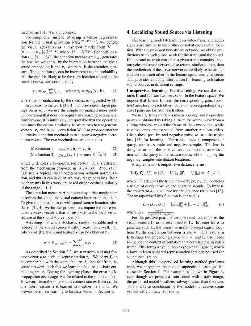
These results can be explained as follows. In the early

stage, our model mistakenly concludes with false random

output (e.g., activation on the road given car sound). How-

ever, it obtains a good score (as it is paired), thereby the

model is trained to behave similarly for such scenes. It

again reinforces its model to receive good scores in simi-

lar examples. Additionally, in the case of the road example,

the proposed network consistently sees road with similar

car sound during training. Since road has simpler appear-

ance and typically occupies larger regions compared to di-

verse appearance of the car (or non-existence of the car in

the frame), it is difficult for the model to discover the true

causality relationship with the car without supervisory feed-

backs. This ends up biasing toward a certain semantically

unrelated output, as in pigeon superstition problem.

As a simple remedy to this issue, we provide some prior

knowledge with supervisory signals in the semi-supervised

setting and algorithm learns successfully (see the last col-

umn of Figure 3).

Semi-supervised learning. Even a small amount of prior

knowledge may induce better inductive bias [23]. We add a

supervised loss into the proposed network architecture un-

der the semi-supervised learning setting. To this end, we

formulate the semi-supervised loss,

L(fv, f+s , f−s ,α,αGT) =

LU (fv, f+s , f−s ) + λ(αGT) · LS(α,αGT),

(6)

where LU and LS denote unsupervised and supervised

losses respectively, αGT denotes the ground-truth (or ref-

erence) attention map, and λ(·) is a function for control-

ling the data supervision type. The unsupervised loss LU

is same as (5). The supervised loss LS can be the mean

square error or cross entropy loss. Empirically, the pro-

posed model with the cross entropy loss performs slightly

better. The adopted cross entropy loss is defined by

LS(α,αGT) = −X

i↵GT,i log(↵i), (7)

where i denotes the location index of the attention map and

↵GT,i is a binary value. We set λ(x) = 0 if x 2 ;, 1 other-

wise. With this formulation, we can easily adapt the loss to

be either supervised or unsupervised one according to the

existence of αGT for each sample. In addition, (6) can be

directly utilized for the fully supervised training.

5. Experimental Results

For evaluation, we first construct a new sound source lo-

calization dataset which facilitates quantitative and qualita-

tive evaluation. Based on this dataset, we evaluate the ca-

pability of the proposed method with various settings. As

aforementioned, while the proposed network is learned to

Orig. Unsup. Semi.

Figure 3. Semantically unmatched results. We show some of

the cases where proposed network draws false conclusions. We

correct this issue by providing a prior knowledge.

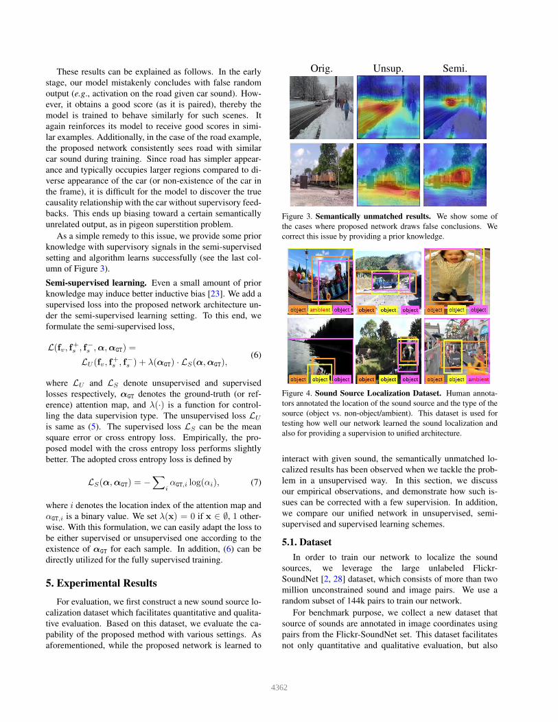
Figure 4. Sound Source Localization Dataset. Human annota-

tors annotated the location of the sound source and the type of the

source (object vs. non-object/ambient). This dataset is used for

testing how well our network learned the sound localization and

also for providing a supervision to unified architecture.

interact with given sound, the semantically unmatched lo-

calized results has been observed when we tackle the prob-

lem in a unsupervised way. In this section, we discuss

our empirical observations, and demonstrate how such is-

sues can be corrected with a few supervision. In addition,

we compare our unified network in unsupervised, semi-

supervised and supervised learning schemes.

5.1. Dataset

In order to train our network to localize the sound

sources, we leverage the large unlabeled Flickr-

SoundNet [2, 28] dataset, which consists of more than two

million unconstrained sound and image pairs. We use a

random subset of 144k pairs to train our network.

For benchmark purpose, we collect a new dataset that

source of sounds are annotated in image coordinates using

pairs from the Flickr-SoundNet set. This dataset facilitates

not only quantitative and qualitative evaluation, but also

4362

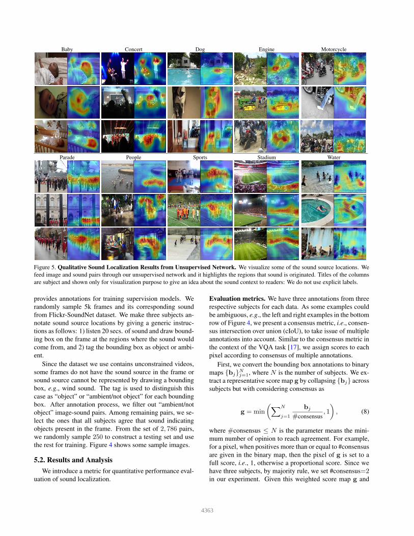
Baby Concert Dog Engine Motorcycle

Parade People Sports Stadium Water

Figure 5. Qualitative Sound Localization Results from Unsupervised Network. We visualize some of the sound source locations. We

feed image and sound pairs through our unsupervised network and it highlights the regions that sound is originated. Titles of the columns

are subject and shown only for visualization purpose to give an idea about the sound context to readers: We do not use explicit labels.

provides annotations for training supervision models. We

randomly sample 5k frames and its corresponding sound

from Flickr-SoundNet dataset. We make three subjects an-

notate sound source locations by giving a generic instruc-

tions as follows: 1) listen 20 secs. of sound and draw bound-

ing box on the frame at the regions where the sound would

come from, and 2) tag the bounding box as object or ambi-

ent.

Since the dataset we use contains unconstrained videos,

some frames do not have the sound source in the frame or

sound source cannot be represented by drawing a bounding

box, e.g., wind sound. The tag is used to distinguish this

case as “object” or “ambient/not object” for each bounding

box. After annotation process, we filter out “ambient/not

object” image-sound pairs. Among remaining pairs, we se-

lect the ones that all subjects agree that sound indicating

objects present in the frame. From the set of 2, 786 pairs,

we randomly sample 250 to construct a testing set and use

the rest for training. Figure 4 shows some sample images.

5.2. Results and Analysis

We introduce a metric for quantitative performance eval-

uation of sound localization.

Evaluation metrics. We have three annotations from three

respective subjects for each data. As some examples could

be ambiguous, e.g., the left and right examples in the bottom

row of Figure 4, we present a consensus metric, i.e., consen-

sus intersection over union (cIoU), to take issue of multiple

annotations into account. Similar to the consensus metric in

the context of the VQA task [17], we assign scores to each

pixel according to consensus of multiple annotations.

First, we convert the bounding box annotations to binary

maps {bj}Nj=1, where N is the number of subjects. We ex-

tract a representative score map g by collapsing {bj} across

subjects but with considering consensus as

g = min

✓

XN

j=1

bj

#consensus, 1

◆

, (8)

where #consensus N is the parameter means the mini-

mum number of opinion to reach agreement. For example,

for a pixel, when positives more than or equal to #consensus

are given in the binary map, then the pixel of g is set to a

full score, i.e., 1, otherwise a proportional score. Since we

have three subjects, by majority rule, we set #consensus=2in our experiment. Given this weighted score map g and

4363

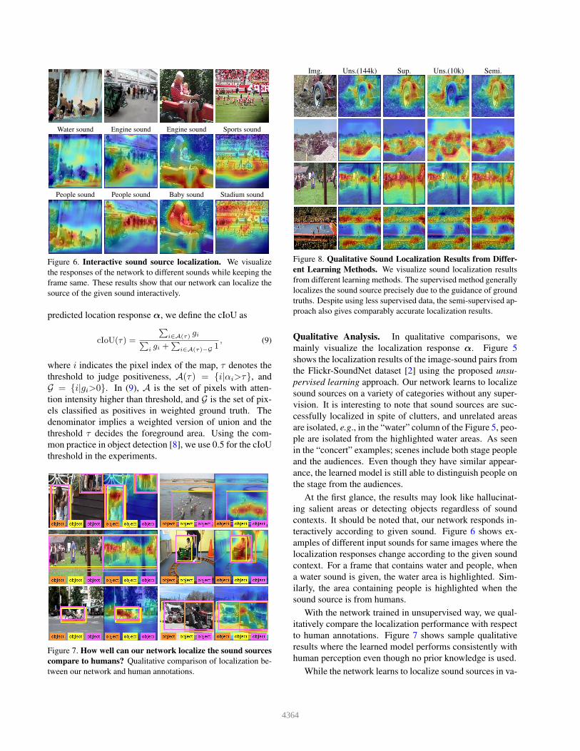
Water sound Engine sound Engine sound Sports sound

People sound People sound Baby sound Stadium sound

Figure 6. Interactive sound source localization. We visualize

the responses of the network to different sounds while keeping the

frame same. These results show that our network can localize the

source of the given sound interactively.

predicted location response α, we define the cIoU as

cIoU(τ) =

Pi∈A(τ) giP

igi +

Pi∈A(τ)−G

1, (9)

where i indicates the pixel index of the map, ⌧ denotes the

threshold to judge positiveness, A(⌧) = {i|↵i>⌧}, and

G = {i|gi>0}. In (9), A is the set of pixels with atten-

tion intensity higher than threshold, and G is the set of pix-

els classified as positives in weighted ground truth. The

denominator implies a weighted version of union and the

threshold ⌧ decides the foreground area. Using the com-

mon practice in object detection [8], we use 0.5 for the cIoU

threshold in the experiments.

Figure 7. How well can our network localize the sound sources

compare to humans? Qualitative comparison of localization be-

tween our network and human annotations.

Img. Uns.(144k) Sup. Uns.(10k) Semi.

Figure 8. Qualitative Sound Localization Results from Differ-

ent Learning Methods. We visualize sound localization results

from different learning methods. The supervised method generally

localizes the sound source precisely due to the guidance of ground

truths. Despite using less supervised data, the semi-supervised ap-

proach also gives comparably accurate localization results.

Qualitative Analysis. In qualitative comparisons, we

mainly visualize the localization response α. Figure 5

shows the localization results of the image-sound pairs from

the Flickr-SoundNet dataset [2] using the proposed unsu-

pervised learning approach. Our network learns to localize

sound sources on a variety of categories without any super-

vision. It is interesting to note that sound sources are suc-

cessfully localized in spite of clutters, and unrelated areas

are isolated, e.g., in the “water” column of the Figure 5, peo-

ple are isolated from the highlighted water areas. As seen

in the “concert” examples; scenes include both stage people

and the audiences. Even though they have similar appear-

ance, the learned model is still able to distinguish people on

the stage from the audiences.

At the first glance, the results may look like hallucinat-

ing salient areas or detecting objects regardless of sound

contexts. It should be noted that, our network responds in-

teractively according to given sound. Figure 6 shows ex-

amples of different input sounds for same images where the

localization responses change according to the given sound

context. For a frame that contains water and people, when

a water sound is given, the water area is highlighted. Sim-

ilarly, the area containing people is highlighted when the

sound source is from humans.

With the network trained in unsupervised way, we qual-

itatively compare the localization performance with respect

to human annotations. Figure 7 shows sample qualitative

results where the learned model performs consistently with

human perception even though no prior knowledge is used.

While the network learns to localize sound sources in va-

4364

0 0.1 0.2 0.3 0.4 0.5 0.6 0.7 0.8 0.9 1

cIoU threshold

0

0.2

0.4

0.6

0.8

1

Su

cce

ss r

atio

Unsup 10k

Unsup 144k

Sup 2.5k

Sup 2.5k + Unsup 10k

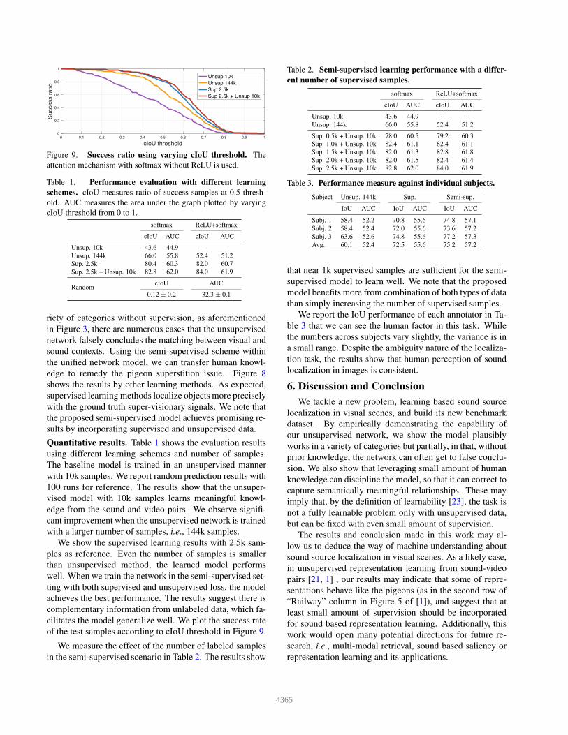
Figure 9. Success ratio using varying cIoU threshold. The

attention mechanism with softmax without ReLU is used.

Table 1. Performance evaluation with different learning

schemes. cIoU measures ratio of success samples at 0.5 thresh-

old. AUC measures the area under the graph plotted by varying

cIoU threshold from 0 to 1.

softmax ReLU+softmax

cIoU AUC cIoU AUC

Unsup. 10k 43.6 44.9 – –

Unsup. 144k 66.0 55.8 52.4 51.2

Sup. 2.5k 80.4 60.3 82.0 60.7

Sup. 2.5k + Unsup. 10k 82.8 62.0 84.0 61.9

RandomcIoU AUC

0.12 ± 0.2 32.3 ± 0.1

riety of categories without supervision, as aforementioned

in Figure 3, there are numerous cases that the unsupervised

network falsely concludes the matching between visual and

sound contexts. Using the semi-supervised scheme within

the unified network model, we can transfer human knowl-

edge to remedy the pigeon superstition issue. Figure 8

shows the results by other learning methods. As expected,

supervised learning methods localize objects more precisely

with the ground truth super-visionary signals. We note that

the proposed semi-supervised model achieves promising re-

sults by incorporating supervised and unsupervised data.

Quantitative results. Table 1 shows the evaluation results

using different learning schemes and number of samples.

The baseline model is trained in an unsupervised manner

with 10k samples. We report random prediction results with

100 runs for reference. The results show that the unsuper-

vised model with 10k samples learns meaningful knowl-

edge from the sound and video pairs. We observe signifi-

cant improvement when the unsupervised network is trained

with a larger number of samples, i.e., 144k samples.

We show the supervised learning results with 2.5k sam-

ples as reference. Even the number of samples is smaller

than unsupervised method, the learned model performs

well. When we train the network in the semi-supervised set-

ting with both supervised and unsupervised loss, the model

achieves the best performance. The results suggest there is

complementary information from unlabeled data, which fa-

cilitates the model generalize well. We plot the success rate

of the test samples according to cIoU threshold in Figure 9.

We measure the effect of the number of labeled samples

in the semi-supervised scenario in Table 2. The results show

Table 2. Semi-supervised learning performance with a differ-

ent number of supervised samples.

softmax ReLU+softmax

cIoU AUC cIoU AUC

Unsup. 10k 43.6 44.9 – –

Unsup. 144k 66.0 55.8 52.4 51.2

Sup. 0.5k + Unsup. 10k 78.0 60.5 79.2 60.3

Sup. 1.0k + Unsup. 10k 82.4 61.1 82.4 61.1

Sup. 1.5k + Unsup. 10k 82.0 61.3 82.8 61.8

Sup. 2.0k + Unsup. 10k 82.0 61.5 82.4 61.4

Sup. 2.5k + Unsup. 10k 82.8 62.0 84.0 61.9

Table 3. Performance measure against individual subjects.

Subject Unsup. 144k Sup. Semi-sup.

IoU AUC IoU AUC IoU AUC

Subj. 1 58.4 52.2 70.8 55.6 74.8 57.1

Subj. 2 58.4 52.4 72.0 55.6 73.6 57.2

Subj. 3 63.6 52.6 74.8 55.6 77.2 57.3

Avg. 60.1 52.4 72.5 55.6 75.2 57.2

that near 1k supervised samples are sufficient for the semi-

supervised model to learn well. We note that the proposed

model benefits more from combination of both types of data

than simply increasing the number of supervised samples.

We report the IoU performance of each annotator in Ta-

ble 3 that we can see the human factor in this task. While

the numbers across subjects vary slightly, the variance is in

a small range. Despite the ambiguity nature of the localiza-

tion task, the results show that human perception of sound

localization in images is consistent.

6. Discussion and Conclusion

We tackle a new problem, learning based sound source

localization in visual scenes, and build its new benchmark

dataset. By empirically demonstrating the capability of

our unsupervised network, we show the model plausibly

works in a variety of categories but partially, in that, without

prior knowledge, the network can often get to false conclu-

sion. We also show that leveraging small amount of human

knowledge can discipline the model, so that it can correct to

capture semantically meaningful relationships. These may

imply that, by the definition of learnability [23], the task is

not a fully learnable problem only with unsupervised data,

but can be fixed with even small amount of supervision.

The results and conclusion made in this work may al-

low us to deduce the way of machine understanding about

sound source localization in visual scenes. As a likely case,

in unsupervised representation learning from sound-video

pairs [21, 1] , our results may indicate that some of repre-

sentations behave like the pigeons (as in the second row of

“Railway” column in Figure 5 of [1]), and suggest that at

least small amount of supervision should be incorporated

for sound based representation learning. Additionally, this

work would open many potential directions for future re-

search, i.e., multi-modal retrieval, sound based saliency or

representation learning and its applications.

4365

References

[1] R. Arandjelovic and A. Zisserman. Look, listen and learn. In

IEEE International Conference on Computer Vision, 2017.

2, 8

[2] Y. Aytar, C. Vondrick, and A. Torralba. Soundnet: Learn-

ing sound representations from unlabeled video. In Neural

Information Processing Systems, 2016. 2, 3, 5, 7

[3] Y. Aytar, C. Vondrick, and A. Torralba. See, hear,

and read: Deep aligned representations. arXiv preprint

arXiv:1706.00932, 2017. 2

[4] D. Bahdanau, K. Cho, and Y. Bengio. Neural machine trans-

lation by jointly learning to align and translate. International

Conference on Learning Representations (ICLR), 2015. 4

[5] Z. Barzelay and Y. Y. Schechner. Harmony in motion. In

IEEE Conference on Computer Vision and Pattern Recogni-

tion, 2007. 3

[6] R. S. Bolia, W. R. D’Angelo, and R. L. McKinley. Aurally

aided visual search in three-dimensional space. Human Fac-

tors, 1999. 2, 3

[7] M. Corbetta and G. L. Shulman. Control of goal-directed

and stimulus-driven attention in the brain. Nature reviews

neuroscience, 2002. 3

[8] M. Everingham, L. Van Gool, C. K. Williams, J. Winn, and

A. Zisserman. The pascal visual object classes (voc) chal-

lenge. International Journal of Computer Vision, 2010. 7

[9] J. W. Fisher III, T. Darrell, W. T. Freeman, and P. A. Vi-

ola. Learning joint statistical models for audio-visual fusion

and segregation. In Neural Information Processing Systems,

2001. 3

[10] A. Frome, G. S. Corrado, J. Shlens, S. Bengio, J. Dean,

T. Mikolov, et al. Devise: A deep visual-semantic embedding

model. In Neural Information Processing Systems, 2013. 2

[11] W. W. Gaver. What in the world do we hear?: An ecological

approach to auditory event perception. Ecological psychol-

ogy, 1993. 1, 2, 3

[12] J. R. Hershey and J. R. Movellan. Audio vision: Using audio-

visual synchrony to locate sounds. In Neural Information

Processing Systems, 1999. 3

[13] E. Hoffer and N. Ailon. Deep metric learning using triplet

network. In International Workshop on Similarity-Based

Pattern Recognition, 2015. 4

[14] H. Izadinia, I. Saleemi, and M. Shah. Multimodal analysis

for identification and segmentation of moving-sounding ob-

jects. IEEE Transactions on Multimedia. 3

[15] D. Jayaraman and K. Grauman. Learning image representa-

tions tied to ego-motion. In IEEE International Conference

on Computer Vision, 2015. 2

[16] B. Jones and B. Kabanoff. Eye movements in auditory space

perception. Attention, Perception, & Psychophysics, 1975.

2, 3

[17] K. Kafle and C. Kanan. Visual question answering: Datasets,

algorithms, and future challenges. Computer Vision and Im-

age Understanding, 2017. 6

[18] E. Kidron, Y. Y. Schechner, and M. Elad. Pixels that sound.

In IEEE Conference on Computer Vision and Pattern Recog-

nition, 2005. 3

[19] P. Majdak, M. J. Goupell, and B. Laback. 3-d localiza-

tion of virtual sound sources: Effects of visual environment,

pointing method, and training. Attention, Perception, & Psy-

chophysics, 2010. 2, 3

[20] A. Owens, P. Isola, J. McDermott, A. Torralba, E. Adelson,

and W. Freeman. Visually indicated sounds. In IEEE Con-

ference on Computer Vision and Pattern Recognition, 2016.

2

[21] A. Owens, W. Jiajun, J. McDermott, W. Freeman, and

A. Torralba. Ambient sound provides supervision for vi-

sual learning. In European Conference on Computer Vision,

2016. 2, 8

[22] D. R. Perrott, J. Cisneros, R. L. McKinley, and

W. R. D’Angelo. Aurally aided visual search under virtual

and free-field listening conditions. 1997. 2, 3

[23] S. Shalev-Shwartz and S. Ben-David. Understanding ma-

chine learning: From theory to algorithms. Cambridge uni-

versity press, 2014. 2, 5, 8

[24] B. R. Shelton and C. L. Searle. The influence of vision on the

absolute identification of sound-source position. Perception

& Psychophysics, 1980. 2, 3

[25] K. Simonyan and A. Zisserman. Very deep convolutional

networks for large-scale image recognition. In International

Conference on Learning Representations, 2015. 3

[26] B. F. Skinner. ”Superstition” in the pigeon. Journal of ex-

perimental psychology, 1948. 2

[27] M. Solr, J. C. Bazin, O. Wang, A. Krause, and A. Sorkine-

Hornung. Suggesting sounds for images from video collec-

tions. In European Conference on Computer Vision Work-

shops, 2016. 2

[28] B. Thomee, D. A. Shamma, G. Friedland, B. Elizalde, K. Ni,

D. Poland, D. Borth, and L. Li. Yfcc100m: The new data in

multimedia research. In Communications of the ACM, 2016.

5

[29] A. Van den Oord, S. Dieleman, and B. Schrauwen. Deep

content-based music recommendation. In Neural Informa-

tion Processing Systems, 2013. 3

[30] H. L. Van Trees. Optimum array processing: Part IV of de-

tection, estimation and modulation theory. Wiley Online Li-

brary, 2002. 3

[31] K. Xu, J. Ba, R. Kiros, K. Cho, A. Courville, R. Salakhutdi-

nov, R. Zemel, and Y. Bengio. Show, attend and tell: Neural

image caption generation with visual attention. In Interna-

tional Conference on Machine Learning, 2015. 3, 4

[32] M. D. Zeiler and R. Fergus. Visualizing and understanding

convolutional networks. In European Conference on Com-

puter Vision, 2014. 3

[33] B. Zhou, A. Khosla, A. Lapedriza, A. Oliva, and A. Tor-

ralba. Learning deep features for discriminative localization.

In IEEE Conference on Computer Vision and Pattern Recog-

nition, 2016. 3, 4

[34] A. Zunino, M. Crocco, S. Martelli, A. Trucco, A. Del Bue,

and V. Murino. Seeing the sound: A new multimodal imag-

ing device for computer vision. In IEEE International Con-

ference on Computer Vision Workshops, 2015. 3

4366