Learning to Disentangle Latent Physical Factorsfor Video Prediction

Deyao Zhu12, Marco Munderloh2, Bodo Rosenhahn2, Jorg Stuckler1

1Max Planck Institute for Intelligent Systems 2Leibniz Universitat Hannover

Abstract. Physical scene understanding is a fundamental human abil-ity. Empowering artificial systems with such understanding is an impor-tant step towards flexible and adaptive behavior in the real world. As astep in this direction, we propose a novel approach to physical scene un-derstanding in video. We train a deep neural network for video predictionwhich embeds the video sequence in a low-dimensional recurrent latentspace representation. We optimize the total correlation of the latent di-mensions within a variational recurrent auto-encoder framework. Thisencourages the representation to disentangle the latent physical factorsof variation in the training data. To train and evaluate our approach,we use synthetic video sequences in three different physical scenarioswith various degrees of difficulty. Our experiments demonstrate that ourmodel can disentangle several appearance-related properties in the unsu-pervised case. If we add supervision signals for the latent code, our modelcan further improve the disentanglement of dynamics-related properties.

1 Introduction

A fundamental ability of humans for understanding dynamic scenes is to perceivephysical properties of objects and predicting the physical evolution of a scenecoarsely into the future. Providing cyber-physical systems with these abilities is akey ingredient to flexible and adaptive behavior in the real word. A large body ofcomputer vision research has recently demonstrated the success of deep learningtechniques for tasks such as object detection and recognition in images or videoprediction. Learning to reason about the dynamic physical states of objects invideo attracts increasing attention recently. A significant part of this researchfocuses on regressing the physical states of the system from images and using aphysics-engine-like module to predict successive frames [28, 2, 25, 30]. Althoughthis is a straightforward approach, it requires hand-crafted tailoring of the staterepresentation and simulator for the specific task. For example, one needs todecide the physical laws to use or the number of represented objects. Somestudies instead directly predict future frames end-to-end using deep learningbased models [31]. Learning latent state representations that disentangle thephysical factors of variation in the data such as object speed, position, mass,and friction, however, is still an open research problem. Such models wouldallow for introspection of the physical properties of a scene.

Accepted for publication in German Conference on Pattern Recognition (GCPR) 2019, to appear

2 D. Zhu, M. Munderloh, B. Rosenhahn, J. Stuckler

In this paper, we propose a variational approach to video prediction thatlearns a recurrent latent representation of the video and allows for predictingsequences into the future. Our network architecture is inspired by state-of-the-art approaches to video prediction [31, 8, 20]. To encourage the learning of adisentangled latent representation we minimize total correlation [4] of the latentdimensions and present videos of varying physical properties during training. Wetrain and evaluate our model on synthetic videos of three physical scenarios withvarying level of difficulty (sliding objects, collision scenarios). Our experimentsdemonstrate that our model can learn to disentangle several appearance-relatedproperties such as shape or size of objects. For various dynamics-related physicalproperties such as speed and friction, we add supervision signals to the latentdimensions and demonstrate that training on total correlation can also improvedisentanglement for these properties. To the best of our knowledge, our workis the first to apply total correlation minimization with the aim of discoveringphysical latent factors in the scene.

The main contributions in this paper are summarized as follows: a) We pro-pose a video prediction model inspired by [31, 8, 20] and train it using totalcorrelation [4]. We also propose an approach to include supervision of dynamics-related properties for representation learning. Our model simultaneously predictsa sequence of future frames and generates latent representations which are phys-ically interpretable for several appearance- and dynamics-related properties. b)We analyze our approach on video datasets of three different physical scenar-ios with increasing difficulty 1. We suggest evaluation metrics for reconstructionquality and disentanglement of latent physical properties for the datasets. c) Weprovide detailed experiments and analysis which demonstrate that our methodoutperforms several variants in our datasets.

2 Related Work

Learning of Physical Scene Understanding: In recent years, the machinelearning community has investigated several approaches to physical scene under-standing [33, 22, 32, 31, 28, 25, 30]. Some approaches attempt to learn the dynam-ics of physical scenes from the explicit state representations (object positions,speed, etc.) which are provided by physics engines [25, 30]. For instance, [25]represents the physical states as a graph and build a learnable and differen-tiable physics engines to update this graph. The approach in [30] introducesa pipeline to predict the next frame with a physics engine in their structure.Visual interaction networks [28] combine recurrent neural networks and interac-tion networks [2] to predict the next physical state. Our approach learns staterepresentations and dynamics models directly from video sequences.

More closely related to our approach, instead of utilizing a physics engineto predict the future state, Ye et al. [31] learn to predict the next frame in anend-to-end way. The proposed architecture is an encoder-decoder network which

1 Dataset available from: https://github.com/TsuTikgiau/DisentPhys4VidPredict

Learning to Disentangle Latent Physical Factors for Video Prediction 3

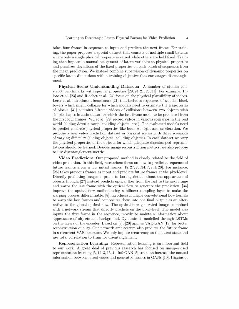
takes four frames in sequence as input and predicts the next frame. For train-ing, the paper proposes a special dataset that consists of multiple small batcheswhere only a single physical property is varied while others are held fixed. Train-ing then imposes a manual assignment of latent variables to physical propertiesand penalizes deviations of the fixed properties on each batch of sequences fromthe mean prediction. We instead combine supervision of dynamic properties onspecific latent dimensions with a training objective that encourages disentangle-ment.

Physical Scene Understanding Datasets: A number of studies con-struct benchmarks with specific properties [29, 24, 21, 23, 31]. For example, Pi-loto et al. [23] and Riochet et al. [24] focus on the physical plausibility of videos.Lerer et al. introduce a benchmark [21] that includes sequences of wooden-blocktowers which might collapse for which models need to estimate the trajectoriesof blocks. [31] contains 5-frame videos of collisions between two objects withsimple shapes in a simulator for which the last frame needs to be predicted fromthe first four frames. Wu et al. [29] record videos in various scenarios in the realworld (sliding down a ramp, colliding objects, etc.). The evaluated models needto predict concrete physical properties like bounce height and acceleration. Wepropose a new video prediction dataset in physical scenes with three scenariosof varying difficulty (sliding objects, colliding objects). In each dataset we varythe physical properties of the objects for which adequate disentangled represen-tations should be learned. Besides image reconstruction metrics, we also proposeto use disentanglement metrics.

Video Prediction: Our proposed method is closely related to the field ofvideo prediction. In this field, researchers focus on how to predict a sequence offuture frames given a few initial frames [18, 27, 26, 34, 7, 8, 1, 20]. For instance,[26] takes previous frames as input and predicts future frames at the pixel-level.Directly predicting images is prone to loosing details about the appearance ofobjects though. [27] instead predicts optical flow from the last to the next frameand warps the last frame with the optical flow to generate the prediction. [34]improve the optical flow method using a bilinear sampling layer to make thewarping process differentiable. [8] introduces multiple convolutional flow kernelsto warp the last frames and composites them into one final output as an alter-native to the global optical flow. The optical flow generated images combinedwith a network stream that directly predicts on the pixel-level. The model alsoinputs the first frame in the sequence, mostly to maintain information aboutappearance of objects and background. Dynamics is modelled through LSTMson the layers of the encoder. Based on [8], [20] applies VAE-GAN [19] for betterreconstruction quality. Our network architecture also predicts the future framein a recurrent VAE structure. We only impose recurrency on the latent state anduse total correlation to train for disentanglement.

Representation Learning: Representation learning is an important fieldto our work. A great deal of previous research has focused on unsupervisedrepresentation learning [5, 12, 3, 15, 4]. InfoGAN [5] trains to increase the mutualinformation between latent codes and generated frames in GANs [10]. Higgins et

4 D. Zhu, M. Munderloh, B. Rosenhahn, J. Stuckler

FirstFrame

CurrentFrame

6

4 x

6

4 x

3

2

3

2 x

3

2 x

6

4

3

2 x

3

2 x

6

4

1

6 x

1

6 x

12

8

1

6 x

1

6 x

12

8

8 x

8 x

25

6

8 x

8 x

25

6

1

6 x

1

6 x

25

6

1

6 x

1

6 x

25

6

3

2 x

3

2 x

12

8

3

2 x

3

2 x

12

8

6

4 x

6

4 x

6

4

12

8 x

12

8 x

3

2

12

8 x

12

8 x

3

21

28

x 1

28

x

32

12

8 x

12

8 x

3

2

WarpedFrame

PredictedNext

Frame

OpticalFlow

GeneratedPixels

Masks

sa

mp

le

late

nt

co

de

Encoder Decoder

Com-posite

warp

Conv

Linear

GRU

Latent Code

10

24

12

8

10

24

64

16

38

4

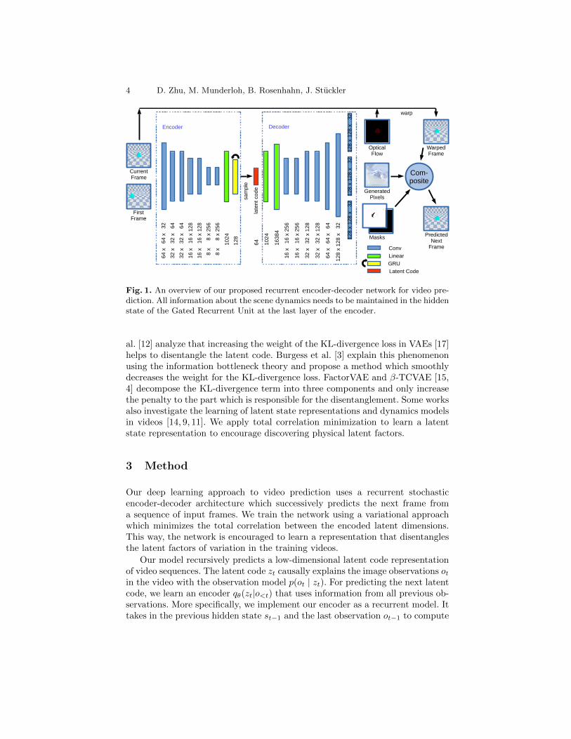
Fig. 1. An overview of our proposed recurrent encoder-decoder network for video pre-diction. All information about the scene dynamics needs to be maintained in the hiddenstate of the Gated Recurrent Unit at the last layer of the encoder.

al. [12] analyze that increasing the weight of the KL-divergence loss in VAEs [17]helps to disentangle the latent code. Burgess et al. [3] explain this phenomenonusing the information bottleneck theory and propose a method which smoothlydecreases the weight for the KL-divergence loss. FactorVAE and β-TCVAE [15,4] decompose the KL-divergence term into three components and only increasethe penalty to the part which is responsible for the disentanglement. Some worksalso investigate the learning of latent state representations and dynamics modelsin videos [14, 9, 11]. We apply total correlation minimization to learn a latentstate representation to encourage discovering physical latent factors.

3 Method

Our deep learning approach to video prediction uses a recurrent stochasticencoder-decoder architecture which successively predicts the next frame froma sequence of input frames. We train the network using a variational approachwhich minimizes the total correlation between the encoded latent dimensions.This way, the network is encouraged to learn a representation that disentanglesthe latent factors of variation in the training videos.

Our model recursively predicts a low-dimensional latent code representationof video sequences. The latent code zt causally explains the image observations otin the video with the observation model p(ot | zt). For predicting the next latentcode, we learn an encoder qθ(zt|o<t) that uses information from all previous ob-servations. More specifically, we implement our encoder as a recurrent model. Ittakes in the previous hidden state st−1 and the last observation ot−1 to compute

Learning to Disentangle Latent Physical Factors for Video Prediction 5

the next hidden state st = fθ(st−1, ot−1). The hidden state st defines a distri-bution �zt ∼ qθ(zt | st) from which the latent code at this step is sampled. Therecurrent autoencoder also requires to learn the observation model pψ(ot | zt)with parameters ψ (the decoder).

3.1 Learning Objective

For training this model, we derive a variational lower bound similar to the vari-ational autoencoder [17] and PlaNet [11]. We maximize the data likelihood ofthe image observations in the video,

ln p(o1:T ) = ln�

t

�p(ot | zt)p(zt | ot−1, st−1)dzt

≥�

t

Eqθ(zt|ot−1,st−1) [ln p(ot | zt)]� �� �−Lrec,t

−KL(qθ(zt | ot−1, st−1) || p(zt | ot−1, st−1))� �� �LKL,t

,

(1)

where we assume an uninformed Gaussian prior with zero mean and unit diag-onal covariance for the state-transition model p(zt | ot−1, st−1). By this approx-imation, we can use techniques such as β-VAE and β-TCVAE to encourage thelatent code to disentangle the latent factors of variation in the training data.The derivation of Eq. 1 can be found in the supplementary material.

The ELBO decomposes in a reconstruction Lrec,t and a complexity term

LKL,t per time step. We use the Laplace distribution 12b exp(−

|x−x|b ) with fixed

scale parameter b as the output distribution of decoder. By this, the reconstruc-tion loss can be written as Lrec,t =

1b

� |xt − xt|, where xt denotes the groundtruth frame and xt is the predicted frame. The KL-divergence term can be de-termined in closed form, since our encoder predicts a normal distribution withdiagonal covariance.

The final training objective for our VAE model is

LVAE = Lrec + LKL, (2)

where Lrec =�

t Lrec,t and LKL =�

t LKL,t.Recent representation learning approaches have demonstrated that augmen-

tations to this loss function can improve the disentanglement of the represen-tation into the latent factors of variation in the training data. β-VAE increasesthe penalty to the KL-divergence term,

Lβ−VAE = Lrec + βLKL. (3)

Here, β > 1. β-TCVAE instead decomposes the KL-divergence term into threecomponents

LKL,t = KL(q(ot−1, zt | st−1) � p(ot−1 | st−1)q(zt | st−1))

+ KL(q(zt | st−1) ��

i

q(zt,i | st−1)) +�

i

KL(q(zt,i | st−1) � p(zt,i))

(4)

6 D. Zhu, M. Munderloh, B. Rosenhahn, J. Stuckler

and only increases the penalty to the total correlation KL(q(zt | st−1) ��

i q(zt,i |st−1)) which is mainly responsible for disentanglement as explained in [4].

Supervision of Latent Dimensions: We also explore training specificdimensions of our latent representation in a supervised way. For selected prop-erties, we normalize their values to the range [−10, 10] and impose an L1 lossbetween them and specific dimensions of the latent code as an additional lossterm. The final training objective in this case is,

Lsup = Lunsup + λ�

t

�

i

|ft,i − �zt,i|. (5)

Here, Lunsup is either LVAE or Lβ−VAE , ft,i is the value of the i-th propertyto be supervised at time step t, and �zt,i is the corresponding dimension of thelatent code sample.

3.2 Network Structure

Our encoder is a recurrent neural network which receives the last hidden statest−1, the latest image ot−1 and the first image o1 in the sequence. It outputsa prediction for the state st of the next frame which we interpret and splitinto the mean and diagonal log variances of a normal distribution qθ(zt|st) =qθ(zt|st−1, ot−1). The decoder deconvolves samples from the encoder distributioninto a Laplace distribution over the pixels in the predicted image. In Fig. 1 wegive an overview and details of our network structure.

Besides the last frame, the encoder also takes in the first frame as input fora better conditioning of the reconstruction of background and object shapes.To remember information from previous steps, a GRU [6] layer is used for thelast layer of the encoder. Note that the current output of the GRU layer is alsoits hidden state for the next step (unlike in an LSTM [13]). By this, the modelneeds to store all information about dynamics in the latent code distribution.

The decoder takes the latent code sample from the encoder and assemblesit into the predicted next frame. It first generates a shared feature map via anupsampling network. Then, three small nets convert the shared feature map intooptical flow, generated pixels and masks, respectively. The optical flow is usedto warp the last frame towards the next frame. Warped frame and generatedpixels are composed together via the masks to yield the predicted next frame.

For better image quality, adding skip connections between encoder and de-coder or adding recurrency into the decoder are effective approaches [8, 20, 7].However, these approaches circumvent the representational bottleneck in the la-tent code and can store dynamics information in other layers. Since we aim at alatent code that represents the appearance and dynamics information requiredto predict the next frame, we don’t adopt these approaches.

Our model takes the first and current frame as input to predict the nextframe in each step. The current frame can be either the ground truth data orthe predicted one from the last step. At the beginning of the sequence, we feedour model four consecutive ground truth frames to initialize the hidden state

Learning to Disentangle Latent Physical Factors for Video Prediction 7

Fig. 2. Samples from our datasets. Row 1, 2, 3 are from the sliding set, the wall setand the collision set, respectively.

of the recurrent encoder. Then, the system recursively uses the predicted imagefrom the last step to perform multi-step prediction.

4 Physical Scene Datasets

We evaluate our approach in videos of physical scenarios of increasing difficulty.We employ the physics engine PyBullet to create three datasets. In the slidingset, objects of various shapes and friction coefficients slide with various initialspeeds on a plane. The wall set shows collisions of a sliding object with a wall.The collision set contains collision scenarios of two objects that slide into eachothers. In the latter two, we also vary the density and the restitution coefficientsof objects. Example sequences for the datasets are shown in Fig. 2.

For each sequence, we record 10 frames with a rate of 10Hz. Besides, segmen-tation masks and depth maps are saved, too. The objects in our dataset have5 different shapes: cylinder, prism, cube, cone and pyramid. The ratios amongedges are fixed, but the scales of objects are changeable for the diversity of data.

Sliding Dataset: The sliding dataset describes a physics scene where anobject with various appearances and physical properties slides from left to theright. We do not include sequences in which the object would fall over. Objects inthis dataset have 5 properties: shape, scale, friction coefficient, initial speed, andinitial position. Different sequences have different combination of these propertieswhich we choose from a finite set of discrete values per property. The set totallyhas 26000 sequences including a training set with 20000 sequences, a validationset with 3000 sequences, and a test set with 3000 sequences.

Wall Dataset: Similar to the sliding dataset, the objects in the wall datasetalso slide from left to the right. However, the object slides into a fixed wall inthe right of the scene. If the object is fast enough, it will hit the wall and bounceback. In this dataset, objects may also fall over. We have 5 properties in this set:shape, scale, material, initial speed, and initial position. Each material has itsown setting of density, restitution, friction, and color. Again we choose a discreteset of possible values for each property. We have totally 10125 sequences in this

8 D. Zhu, M. Munderloh, B. Rosenhahn, J. Stuckler

GT

Pred

Fig. 3. Prediction examples of β-TCVAE in different datasets. First row demonstratesthe ground truth frames. Second row shows the 1st (t = 5), 3rd, and 5th predictedframes in three datasets.

set including 7425 sequenes in the training set, 1350 in the validation set and1350 in the test set.

Collision Dataset: In the collision dataset, 2 objects slide into each otherfrom left and right. Both objects have their own settings of shapes, scales, ma-terials, initial speeds and positions from a discrete set of values. This set has25000 sequences in the training set, 2500 sequences in the validation set and2500 sequences in the test set.

5 Experiments

We evaluate our video representation learning approach on our proposed datasets.To measure the level of the latent code’s disentanglement we use the mutual in-formation gap (MIG) proposed in [4]. We also measure the disentanglement ofa property separately by computing the mutual information gap for the singleproperty. Additionally, we assess the quality of the video prediction using thepeak signal-to-noise ratio (PSNR).

Experiments for Unsupervised Learning: We first assess unsupervisedlearning with our approach and compare VAE, β-VAE [12] and β-TCVAE [4]objectives for various β values. The models are trained to predict the remainingsix frames in each sequence given the first four ground truth frames as inputs.

To explore the relationship between the coefficient β and the level of disen-tanglement, we evaluate a set of β values. In the sliding set, we set β to 1, 5, 9,13, 17, 21, 25; in the wall and the collision set, β are set to 1, 6, 11, 16, 21, 26 and1, 11, 21, 31, respectively. Each setting is trained 22 times in the sliding set and12 times in the other sets. Each model is trained for 12000 iterations. We usethe Adam optimizer [16] with parameters β1 = 0.5, β2 = 0.999 and learning rate6e−9. Batch size is set to 8. For the scale parameter of the decoder’s Laplacedistribution we empirically choose b = 0.0147. Schedule sampling [8] is appliedfor training: The model is first trained to predict only one future step at thebeginning of training. Then we smoothly transition to full sequence predictionfrom iteration 1000 to iteration 9000.

Some prediction examples of β-TCVAE are given in Fig. 3. The averageMIG curves are shown in Fig. 4 (a) (b) (c). We show means and 90% confidenceintervals of evaluated MIG values. For the sliding set and wall set, a higher β

Learning to Disentangle Latent Physical Factors for Video Prediction 9

� � �� �� �� ������

����

����

����

����

����

����

���

(a) Slide - Average MIG

� � �� �� �� ������

����

����

����

����

����

���

(b) Wall - Average MIG

� � �� �� �� �� ������

����

����

����

����

����

����

���

(c) Collision - Average MIG

0� 5� 10� 15� 20� 25�beta�28.0�

28.5�

29.0�

29.5�

30.0�

PSNR�

(d) Sliding - PSNR

0� 5� 10� 15� 20� 25� beta�

31.5�

32.0�

32.5�

33.0�PSNR�

(e) Wall - PSNR

0� 5� 10� 15� 20� 25� 30� beta�24.5�

25.0�

25.5�

26.0�

26.5�

PSNR�

beta-VAE �beta-TCVAE�

(f) Collision - PSNR

Fig. 4. MIG and performance reduction (average and 90% confidence intervals) forunsupervised learning. In the sliding set and the wall set, β-TCVAE outperforms β-VAEand successfully increase the average MIG. Besides, larger β leads to bigger performancereduction in both approahces.

GT VAE β-VAE β-TCVAE GT VAE β-VAE β-TCVAE

Fig. 5. Predicted last frame of two sequences for different approaches.

helps to increase the average MIG in β-TCVAE. In contrast, β-VAE strugglesto improve it. For the most difficult collision set, β-TCVAE slightly improvesover β-VAE, while there is no obvious improvement over VAE (β = 1). Largerβ values limit the capacity of the model by forcing it to stay closer to the priorwhich negatively influences the video prediction quality. This can be seen inFig. 4 (d) (e) (f) in the reduction in PSNR. We observe that the reduction for β-TCVAE is smaller than for β-VAE in most cases. Fig. 5 shows the last predictedframe in a video sequence by the different approaches.

To figure out which kinds of properties benefit from a larger β, we presentthe MIGs for individual properties in Fig. 6. Both β-TCVAE and β-VAE candisentangle some properties better like shapes in the sliding set or position in thecollision set. β-TCVAE achieves better results than β-VAE. However, the ap-proaches struggle to disentangle dynamic-related properties like speed or friction.To visualize the results of β-TCVAE and β-VAE, we select our best β-TCVAE,β-VAE and VAE (β = 1) models and show latent traversals for shapes in thesliding set in Fig. 7. For the traversals, we select the dimension of the latent codethat has the highest mutual information with the shape.

Experiments for Supervised Learning: Although unsupervised learningin our model using the β-TCVAE objective can improve the disentanglement

10 D. Zhu, M. Munderloh, B. Rosenhahn, J. Stuckler

� � �� �� �� ������

���

���

���

���

���

��������

�����

�����

��������

�����

��������

(a) Sliding - β-VAE

� � �� �� �� ������

���

���

���

���

���

������

��������

�����

�����

��������

�����

��������

(b) Wall - β-VAE

� � �� �� �� �� �� ��������

����

����

����

����

�������

������������������������������������������������������������������������������������������

(c) Collision - β-VAE

� � �� �� �� ������

���

���

���

���

���

��������

�����

�����

��������

�����

��������

(d) Sliding - β-TCVAE

� � �� �� �� ������

���

���

���

���

���

������

��������

�����

�����

��������

�����

��������

(e) Wall - β-TCVAE

� � �� �� �� �� �� ��������

����

����

����

����

�������

������������������������������������������������������������������������������������������

(f) Collision - β-TCVAE

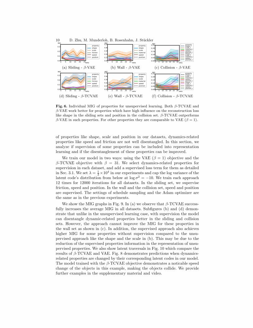
Fig. 6. Individual MIG of properties for unsupervised learning. Both β-TCVAE andβ-VAE work better for properties which have high influence on the reconstruction losslike shape in the sliding sets and position in the collision set. β-TCVAE outperformsβ-VAE in such properties. For other properties they are comparable to VAE (β = 1).

of properties like shape, scale and position in our datasets, dynamics-relatedproperties like speed and friction are not well disentangled. In this section, weanalyze if supervision of some properties can be included into representationlearning and if the disentanglement of these properties can be improved.

We train our model in two ways: using the VAE (β = 1) objective and theβ-TCVAE objective with β = 31. We select dynamics-related properties forsupervision in each dataset, and add a supervised loss term for them as detailedin Sec. 3.1. We set λ = 1

3×104 in our experiments and cap the log variance of thelatent code’s distribution from below at log σ2 = −10. We train each approach12 times for 12000 iterations for all datasets. In the sliding set, we supervisefriction, speed and position. In the wall and the collision set, speed and positionare supervised. The settings of schedule sampling and the Adam optimizer arethe same as in the previous experiments.

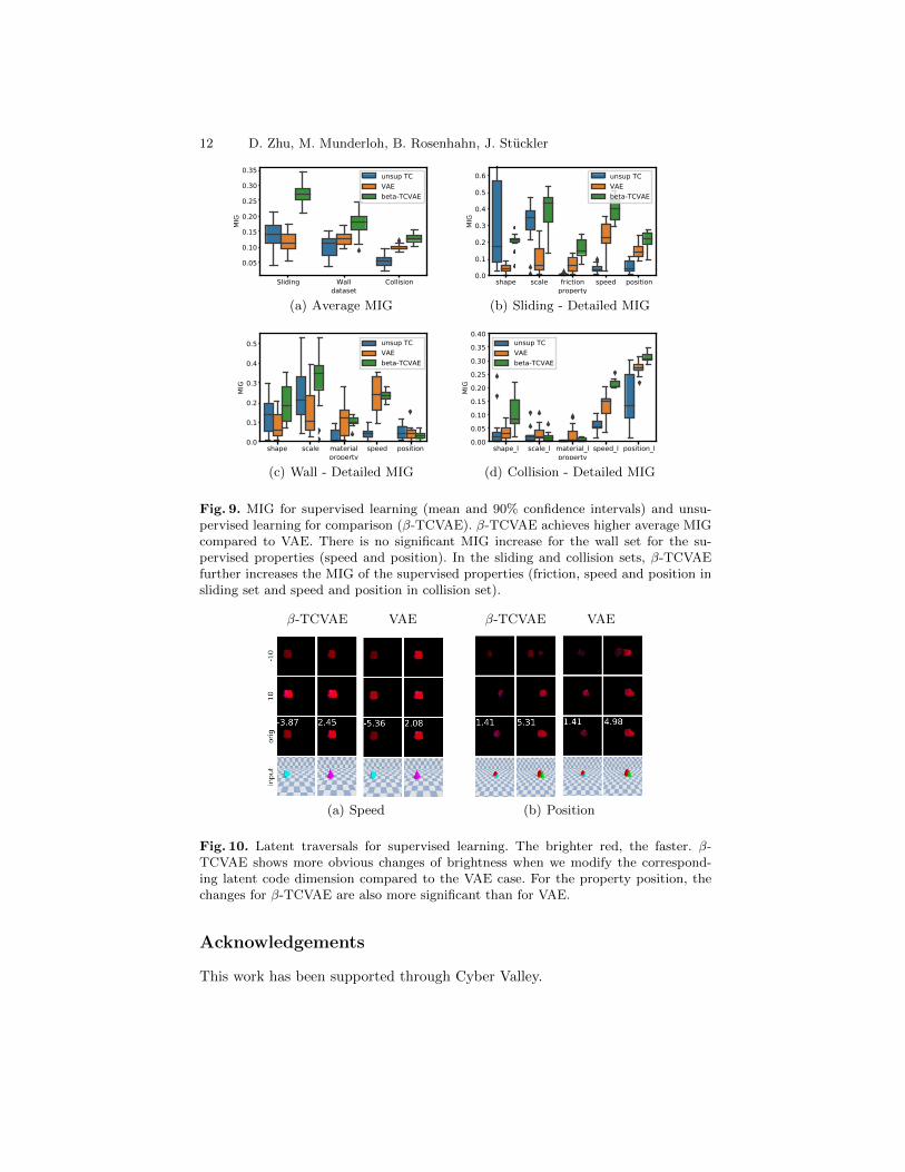
We show the MIG graphs in Fig. 9. In (a) we observe that β-TCVAE success-fully increases the average MIG in all datasets. Subfigures (b) and (d) demon-strate that unlike in the unsupervised learning case, with supervision the modelcan disentangle dynamic-related properties better in the sliding and collisionsets. However, the approach cannot improve the MIG for these properties inthe wall set as shown in (c). In addition, the supervised approach also achieveshigher MIG for some properties without supervision compared to the unsu-pervised approach like the shape and the scale in (b). This may be due to thereduction of the supervised properties information in the representation of unsu-pervised properties. We also show latent traversals in Fig. 10 which compare theresults of β-TCVAE and VAE. Fig. 8 demonstrates predictions when dynamics-related properties are changed by their corresponding latent codes in our model.The model trained with the β-TCVAE objective demonstrates a noticable speedchange of the objects in this example, making the objects collide. We providefurther examples in the supplementary material and video.

Learning to Disentangle Latent Physical Factors for Video Prediction 11

(a) β-TCVAE (b) β-VAE (c) VAE

Fig. 7. Latent traversals for the shape property in the sliding set. We manually modifythe value (given in row headers) of the dimension corresponding to the specific prop-erty and show the predicted optical flows in the first 2 rows. The orig row shows theprediction for the estimated value of the dimension. In the first 2 examples, the contourchanges from a triangle-like shape to a rectangular-like shape as we increase the valuein β-TCVAE and β-VAE models while this is not the case for standard VAE.

ground truth original prediction modified predicition

TCVAE

VAE

Fig. 8. Effect of latent code modification. We show predicted 1st and last frames fromβ-TCVAE and VAE. In the last column, we modified the latent code dimension cor-responding to the speed at t = 4 and show subsequent predicitions. While β-TCVAEgenerates a collision event, there is only little change for VAE.

6 Conclusion

In this paper, we propose a recurrent variational autoencoder model that learnsa latent dynamics representation for video prediction. We use total correlationto improve the disentanglement of the learned representation into the latent fac-tors of variation in the training data. In this way, the model can discover severalproperties related to the physics of the scenarios such as shape or positions ofobjects. We also demonstrate that partial supervision of dynamics-related prop-erties can be added which further improves the disentanglement of the represen-tation. We evaluate our approach on a new dataset of three physical scenarioswith increasing levels of difficulty. In future work we plan to extend our datasetto more complex scenarios and investigate other network architectures to furtherimprove the level of scene understanding.

12 D. Zhu, M. Munderloh, B. Rosenhahn, J. Stuckler

������� ���� ���������

�������

����

����

����

����

����

����

����

���

��������

���

����������

(a) Average MIG

����� ����� �������� ����� ��������

��������

���

���

���

���

���

���

���

���

��������

���

����������

(b) Sliding - Detailed MIG

����� ����� �������� ����� ��������

��������

���

���

���

���

���

���

���

��������

���

����������

(c) Wall - Detailed MIG

������� ������� ���������� ������� ����������

��������

����

����

����

����

����

����

����

����

����

���

��������

���

����������

(d) Collision - Detailed MIG

Fig. 9. MIG for supervised learning (mean and 90% confidence intervals) and unsu-pervised learning for comparison (β-TCVAE). β-TCVAE achieves higher average MIGcompared to VAE. There is no significant MIG increase for the wall set for the su-pervised properties (speed and position). In the sliding and collision sets, β-TCVAEfurther increases the MIG of the supervised properties (friction, speed and position insliding set and speed and position in collision set).

β-TCVAE VAE β-TCVAE VAE

(a) Speed (b) Position

Fig. 10. Latent traversals for supervised learning. The brighter red, the faster. β-TCVAE shows more obvious changes of brightness when we modify the correspond-ing latent code dimension compared to the VAE case. For the property position, thechanges for β-TCVAE are also more significant than for VAE.

Acknowledgements

This work has been supported through Cyber Valley.

Learning to Disentangle Latent Physical Factors for Video Prediction 13

References

1. Babaeizadeh, M., Finn, C., Erhan, D., Campbell, R., Levine, S.: Stochastic varia-tional video prediction. In: International Conference on Learning Representations(ICLR) (2018)

2. Battaglia, P., Pascanu, R., Lai, M., Rezende, D., Kavukcuoglu, K.: Interactionnetworks for learning about objects, relations and physics. In: Advances in NeuralInformation Processing Systems (NIPS) (2016)

3. Burgess, C., Higgins, I., Pal, A., Matthey, L., Watters, N., Desjardins, G., Lerch-ner, A.: Understanding disentangling in beta-vae. In: NIPS Workshop on LearningDisentangled Representations (2017)

4. Chen, T., Li, X., Grosse, R., Duvenaud, D.: Isolating sources of disentanglementin vaes. In: Advances in Neural Information Processing Systems (NIPS) (2018)

5. Chen, X., Duan, Y., Houthooft, R., Schulman, J., Sutskever, I., Abbeel, P.: Info-GAN: Interpretable representation learning by information maximizing generativeadversarial nets. In: Advances in Neural Information Processing Systems (NIPS)(2016)

6. Chung, J., Gulcehre, C., Cho, K., Bengio, Y.: Empirical evaluation of gated recur-rent neural networks on sequence modeling. In: NIPS Workshop on Deep Learningand Representation Learning (2014)

7. Ebert, F., Finn, C., Lee, X., Levine, S.: Self-supervised visual planning with tem-poral skip connections. In: International Conference on Robot Learning (CoRL)(2017)

8. Finn, C., Goodfellow, I., Levine, S.: Unsupervised learning for physical interactionthrough video prediction. In: Advances in Neural Information Processing Systems(NIPS) (2016)

9. Fraccaro, M., Kamronn, S., Paquet, U., Winther, O.: A disentangled recognitionand nonlinear dynamics model for unsupervised learning. In: Advances in NeuralInformation Processing Systems (NIPS) (2017)

10. Goodfellow, I., Pouget-Abadie, J., Mirza, M., Xu, B., Warde-Farley, D., Ozair,S., Courville, A., Bengio, Y.: Generative adversarial nets. In: Advances in NeuralInformation Processing Systems (NIPS) (2014)

11. Hafner, D., Lillicrap, T., Fischer, I., Villegas, R., Ha, D., Lee, H., Davidson, J.:Learning latent dynamics for planning from pixels. In: Proceedings of the 36thInternational Conference on Machine Learning (ICML). pp. 2555–2565 (2019)

12. Higgins, I., Matthey, L., Pal, A., Burgess, C., Glorot, X., Botvinick, M., Mohamed,S., Lerchner, A.: beta-VAE: Learning basic visual concepts with a constrainedvariational framework. In: International Conference on Learning Representations(ICLR) (2017)

13. Hochreiter, S., Schmidhuber, J.: Convolutional LSTM network: A machine learningapproach for precipitation nowcasting. In: Neural computation (1997)

14. Johnson, M., Duvenaud, D.K., Wiltschko, A., Adams, R.P., Datta, S.R.: Compos-ing graphical models with neural networks for structured representations and fastinference. In: Advances in Neural Information Processing Systems 29 (NIPS), pp.2946–2954 (2016)

15. Kim, H., Mnih, A.: Disentangling by factorising. CoRR abs/1802.05983 (2018)

16. Kingma, D., Ba, J.: Adam: A method for stochastic optimization. In: InternationalConference on Learning Representations (ICLR) (2015)

17. Kingma, D., Welling, M.: Auto-encoding variational bayes (2014)

14 D. Zhu, M. Munderloh, B. Rosenhahn, J. Stuckler

18. Kitani, K., Ziebart, B., Bagnell, J., Hebert, M.: Activity forecasting. In: EuropeanConference on Computer Vision (ECCV) (2012)

19. Larsen, A., Snderby, S., Larochelle, H., Winther, O.: Autoencoding beyond pixelsusing a learned similarity metric. In: International Conference on Machine Learning(ICML) (2016)

20. Lee, X., Zhang, R., Ebert, F., Abbeel, P., Finn, C., Levine, S.: Stochastic adver-sarial video prediction. CoRR abs/1804.01523 (2018)

21. Lerer, A., Gross, S., Fergus, R.: Learning physical intuition of block towers byexample. In: International Conference on Machine Learning (ICML) (2016)

22. Mottaghi, R., Bagherinezhad, H., Rastegari, M., Farhadi, A.: Newtonian sceneunderstanding: Unfolding the dynamics of objects in static images. In: InternationalConference on Computer Vision and Pattern Recognition (CVPR) (2016)

23. Piloto, L., Weinstein, A., T.B., D., Ahuja, A., Mirza, M., Wayne, G., Amos, D.,Hung, C.C., Botvinick, M.: Probing physics knowledge using tools from develop-mental psychology. CoRR 1804.01128 (2018)

24. Riochet, R., Castro, M.Y., Bernard, M., Lerer, A., Fergus, R., Izard, V., Dupoux,E.: IntPhys: A framework and benchmark for visual intuitive physics reasoning.CoRR abs/1803.07616 (2018)

25. Sanchez-Gonzalez, A., Heess, N., Springenberg, J., Merel, J., Riedmiller, M., Had-sell, R., Battaglia, P.: Graph networks as learnable physics engines for inferenceand control. In: International Conference on Machine Learning (ICML) (2018)

26. Srivastava, N., Mansimov, E., Salakhutdinov, R.: Unsupervised learning of videorepresentations using LSTMs. In: International Conference on Machine Learning(ICML) (2015)

27. Walker, J., Doersch, C., Gupta, A., Hebert, M.: An uncertain future: Forecast-ing from variational autoencoders. In: European Conference on Computer Vision(ECCV) (2016)

28. Watters, N., Tacchetti, A., Weber, T., Pascanu, R., Battaglia, P., Zoran, D.: Vi-sual interaction networks. In: Advances in Neural Information Processing Systems(NIPS) (2017)

29. Wu, J., Lim, J.J., Zhang, H., Tenenbaum, J.B., Freeman, W.T.: Physics 101: Learn-ing physical object properties from unlabeled videos. In: British Machine VisionConference (BMVC) (2016)

30. Wu, J., Lu, E., Kohli, P., Freeman, W., Tenenbaum, J.: Learning to see physicsvia visual de-animation. In: Advances in Neural Information Processing Systems(NIPS) (2017)

31. Ye, T., Wang, X., Davidson, J., Gupta, A.: Interpretable intuitive physics model.In: European Conference on Computer Vision (ECCV). pp. 89–105 (2018)

32. Zhang, R., Wu, J., Zhang, C., Freeman, W., Tenenbaum, J.: A comparative evalua-tion of approximate probabilistic simulation and deep neural networks as accountsof human physical scene understanding. In: Annual Conference of the CognitiveScience Society (2016)

33. Zheng, B., Zhao, Y., Yu, J., Ikeuchi, K., Zhu, S.: Scene understanding by reasoningstability and safety. International Journal of Computer Vision (IJCV) 112(2), 221–238 (2015)

34. Zhou, T., Tulsiani, S., Sun, W., Malik, J., Efros, A.: View synthesis by appearanceflow. In: European Conference on Computer Vision (ECCV) (2016)