Learning Probabilistic models for Graph Partitioning with Noise · 2019-06-27 · Graph...
43
Learning Probabilistic models for Graph Partitioning with Noise Based on joint works with Aravindan Vijayaraghavan Northwestern University Yury Makarychev Toyota Technological Institute at Chicago Konstantin Makarychev Microsoft Research
Transcript of Learning Probabilistic models for Graph Partitioning with Noise · 2019-06-27 · Graph...
Learning Probabilistic models for Graph Partitioning with Noise
Based on joint works with
Aravindan Vijayaraghavan
Northwestern University
Yury MakarychevToyota Technological Institute
at Chicago
Konstantin Makarychev
Microsoft Research
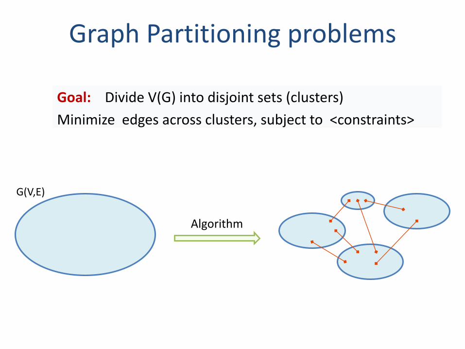
Graph Partitioning problems
Goal: Divide V(G) into disjoint sets (clusters)
Minimize edges across clusters, subject to <constraints>
G(V,E)
Algorithm
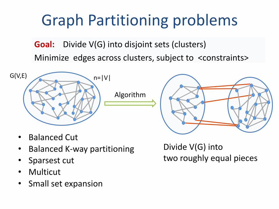
Graph Partitioning problems
Goal: Divide V(G) into disjoint sets (clusters)
Minimize edges across clusters, subject to <constraints>
• Balanced Cut
G(V,E)
Algorithm
• Balanced K-way partitioning• Sparsest cut• Multicut• Small set expansion
Divide V(G) into two roughly equal pieces
n=|V|
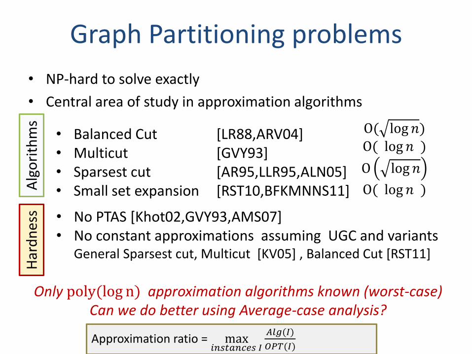
Graph Partitioning problems
• NP-hard to solve exactly
• Central area of study in approximation algorithms
• Balanced Cut • Multicut• Sparsest cut • Small set expansion
Only poly(log n) approximation algorithms known (worst-case)Can we do better using Average-case analysis?
[LR88,ARV04][GVY93][AR95,LLR95,ALN05][RST10,BFKMNNS11]
O( log 𝑛)
O( log 𝑛 )
O log 𝑛
O( log 𝑛 )
• No PTAS [Khot02,GVY93,AMS07]• No constant approximations assuming UGC and variants
General Sparsest cut, Multicut [KV05] , Balanced Cut [RST11]
Alg
ori
thm
sH
ard
nes
s
Approximation ratio = max𝑖𝑛𝑠𝑡𝑎𝑛𝑐𝑒𝑠 𝐼
𝐴𝑙𝑔(𝐼)
𝑂𝑃𝑇(𝐼)
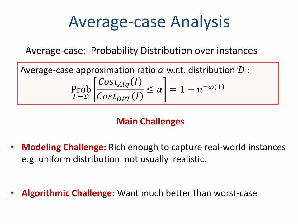
Average-case Analysis
Average-case: Probability Distribution over instances
Average-case approximation ratio 𝛼 w.r.t. distribution 𝒟 :
Prob𝐼 ←𝒟
𝐶𝑜𝑠𝑡𝐴𝑙𝑔 𝐼
𝐶𝑜𝑠𝑡𝑂𝑃𝑇 𝐼≤ 𝛼 = 1 − 𝑛−𝜔(1)
Main Challenges
• Modeling Challenge: Rich enough to capture real-world instances e.g. uniform distribution not usually realistic.
• Algorithmic Challenge: Want much better than worst-case
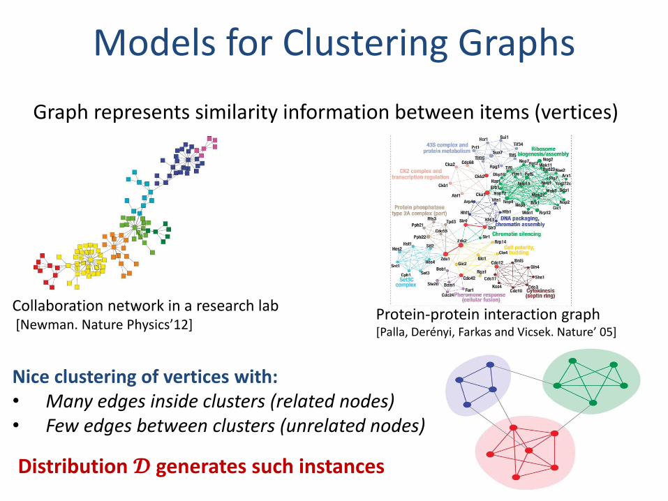
Models for Clustering Graphs
Collaboration network in a research lab[Newman. Nature Physics’12]
Nice clustering of vertices with:• Many edges inside clusters (related nodes)• Few edges between clusters (unrelated nodes)
Protein-protein interaction graph[Palla, Derényi, Farkas and Vicsek. Nature’ 05]
Graph represents similarity information between items (vertices)
Distribution 𝓓 generates such instances
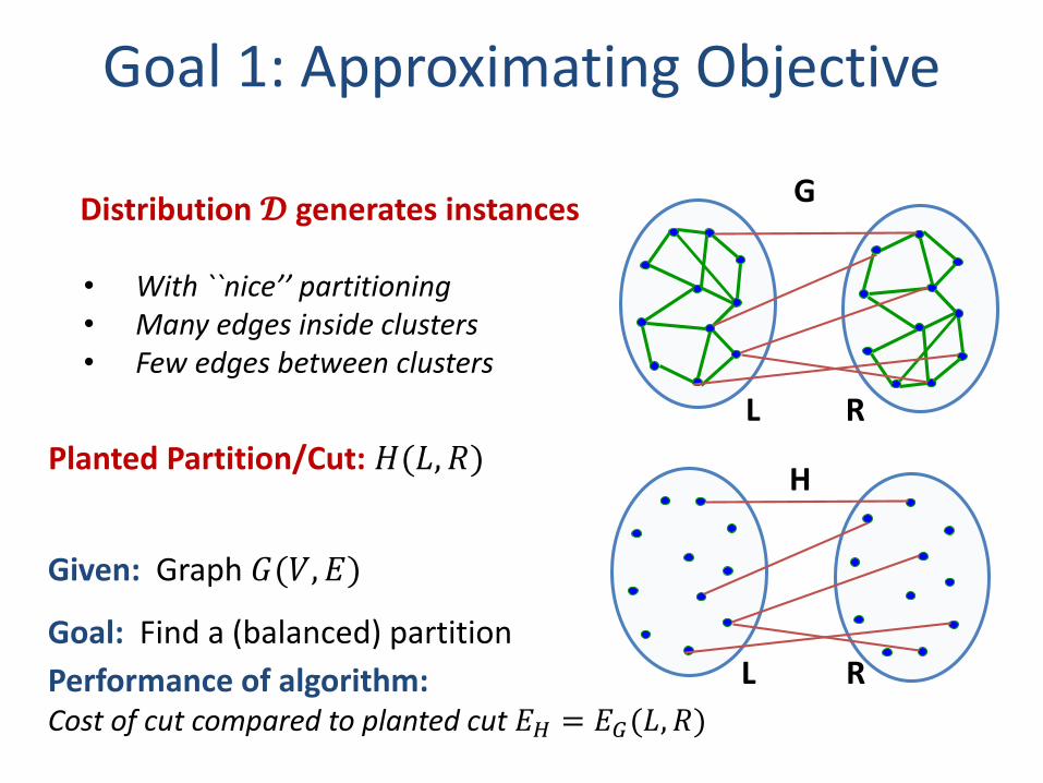
Goal 1: Approximating Objective
• With ``nice’’ partitioning• Many edges inside clusters• Few edges between clusters
Distribution 𝓓 generates instances
RL
G
Planted Partition/Cut: 𝐻(𝐿, 𝑅)
RL
H
Given: Graph 𝐺(𝑉, 𝐸)
Goal: Find a (balanced) partition
Performance of algorithm:Cost of cut compared to planted cut 𝐸𝐻 = 𝐸𝐺(𝐿, 𝑅)
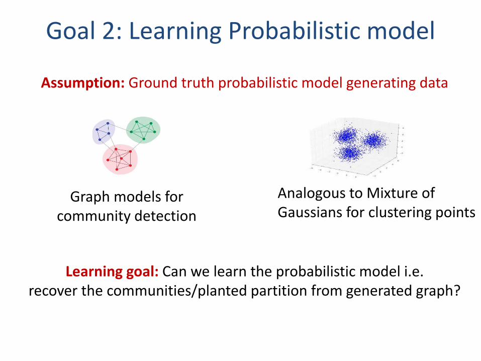
Goal 2: Learning Probabilistic model
Assumption: Ground truth probabilistic model generating data
Learning goal: Can we learn the probabilistic model i.e. recover the communities/planted partition from generated graph?
Analogous to Mixture of Gaussians for clustering points
Graph models for community detection
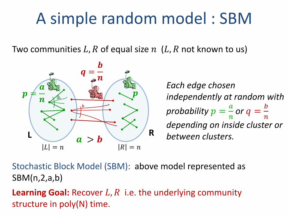
A simple random model : SBM
Two communities 𝐿, 𝑅 of equal size 𝑛 (𝐿, 𝑅 not known to us)
𝒒 =𝒃
𝒏
𝒑 =𝒂
𝒏
RL 𝒂 > 𝒃
Each edge chosen independently at random with
probability 𝑝 =𝑎
𝑛or 𝑞 =
𝑏
𝑛
depending on inside cluster or between clusters.
𝐿 = 𝑛 𝑅 = 𝑛
𝒑
Stochastic Block Model (SBM): above model represented as SBM(n,2,a,b)
Learning Goal: Recover 𝐿, 𝑅 i.e. the underlying community structure in poly(N) time.

Stochastic Block Model 𝑆𝐵𝑀(𝑛, 𝑘, 𝑎, 𝑏)
𝑘 communities of equal size 𝑛. Number of vertices 𝑁 = 𝑛𝑘.
𝒂 > 𝒃
Every edge chosen independently at random.
𝑃𝑖∗ = 𝑛
𝑃𝑗∗ = 𝑛
𝑎= 𝔼ሾdegree of a vertex
Most commonly used probabilistic model for clustering graphs
Number of edges
𝑚 ≈𝑁𝑎
2+
𝑁 𝑘−1 𝑏
2
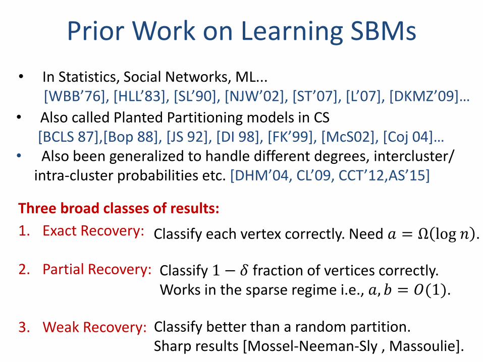
Prior Work on Learning SBMs
• Also called Planted Partitioning models in CS[BCLS 87],[Bop 88], [JS 92], [DI 98], [FK’99], [McS02], [Coj 04]…
• Also been generalized to handle different degrees, intercluster/ intra-cluster probabilities etc. [DHM’04, CL’09, CCT’12,AS’15]
• In Statistics, Social Networks, ML... [WBB’76], [HLL’83], [SL’90], [NJW’02], [ST’07], [L’07], [DKMZ’09]…
Three broad classes of results:
1. Exact Recovery:
2. Partial Recovery:
3. Weak Recovery:
Classify each vertex correctly. Need 𝑎 = Ω log 𝑛 .
Classify better than a random partition. Sharp results [Mossel-Neeman-Sly , Massoulie].
Classify 1 − 𝛿 fraction of vertices correctly. Works in the sparse regime i.e., 𝑎, 𝑏 = 𝑂(1).
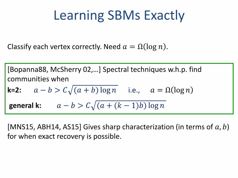
Learning SBMs Exactly
[Bopanna88, McSherry 02,…] Spectral techniques w.h.p. find communities when
k=2: 𝑎 − 𝑏 > 𝐶 (𝑎 + 𝑏) log 𝑛 i.e., 𝑎 = Ω log 𝑛
general k: 𝑎 − 𝑏 > 𝐶 (𝑎 + (𝑘 − 1)𝑏) log 𝑛
[MNS15, ABH14, AS15] Gives sharp characterization (in terms of 𝑎, 𝑏) for when exact recovery is possible.
Classify each vertex correctly. Need 𝑎 = Ω log 𝑛 .
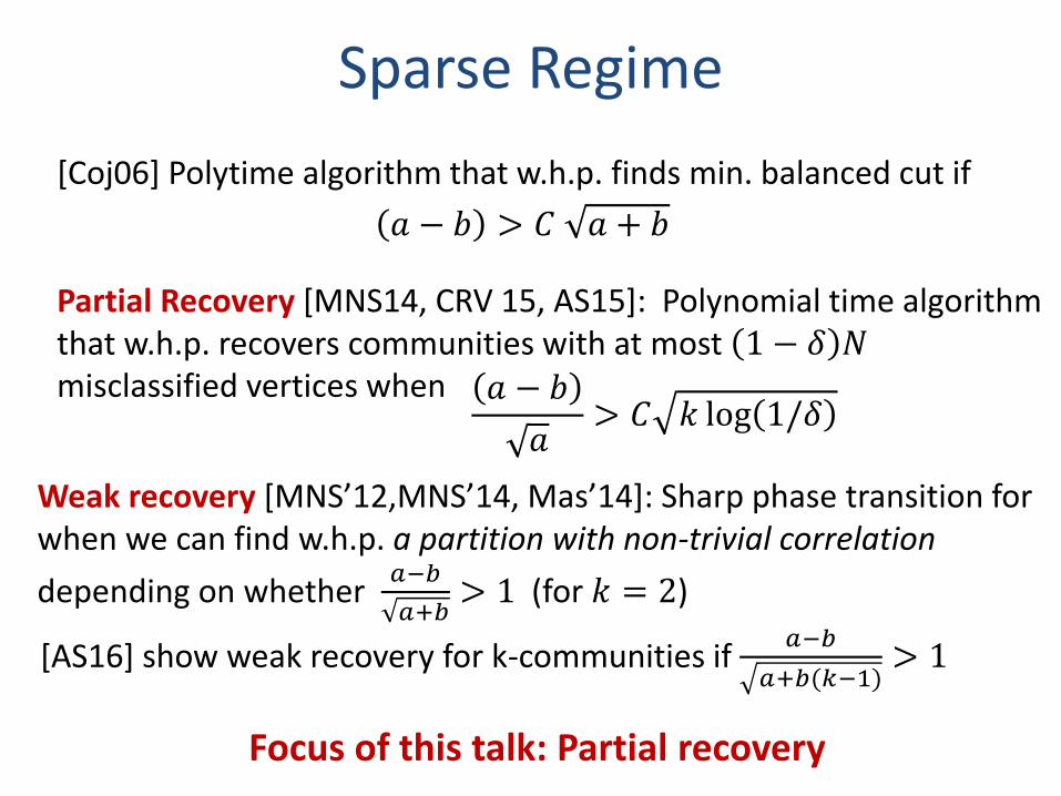
Sparse Regime
[Coj06] Polytime algorithm that w.h.p. finds min. balanced cut if
𝑎 − 𝑏 > 𝐶 𝑎 + 𝑏
Partial Recovery [MNS14, CRV 15, AS15]: Polynomial time algorithm that w.h.p. recovers communities with at most 1 − 𝛿 𝑁misclassified vertices when
Focus of this talk: Partial recovery
𝑎 − 𝑏
𝑎> 𝐶 𝑘 log 1/𝛿
[AS16] show weak recovery for k-communities if 𝑎−𝑏
𝑎+𝑏(𝑘−1)> 1
Weak recovery [MNS’12,MNS’14, Mas’14]: Sharp phase transition for when we can find w.h.p. a partition with non-trivial correlation
depending on whether 𝑎−𝑏
𝑎+𝑏> 1 (for 𝑘 = 2)
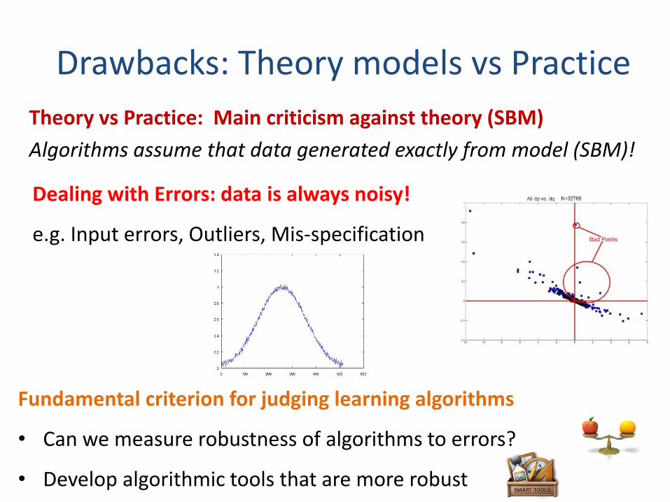
Drawbacks: Theory models vs Practice
Theory vs Practice: Main criticism against theory (SBM)
Algorithms assume that data generated exactly from model (SBM)!
Dealing with Errors: data is always noisy!
e.g. Input errors, Outliers, Mis-specification
Fundamental criterion for judging learning algorithms
• Can we measure robustness of algorithms to errors?
• Develop algorithmic tools that are more robust
How Robust are Usual Approaches?
Spectral clustering: Project and cluster in space spanned by top 𝑘-eigenvectors.
Drawback: Spectral methods are not very robust Eigenvectors brittle to noise: can add & delete just O(1) edges.
• Other algorithms based on counting paths, random walks, tensor methods are also not robust.
Maximum Likelihood (ML) estimation: Find the best fit model measured in KL divergence (measure of closeness for distributions)
Drawback: ML estimation is typically NP-hard!
• Heuristics like EM typically get stuck in local optima.
Drawbacks of Random Models
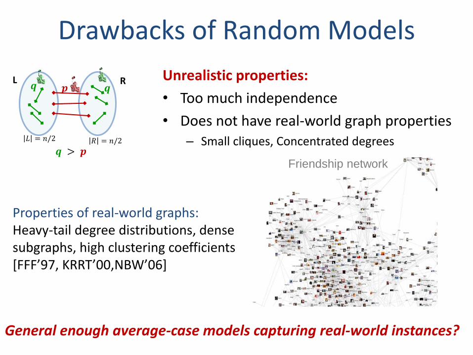
𝒑𝒒 RL
𝒒 > 𝒑
𝐿 = 𝑛/2 𝑅 = 𝑛/2
𝒒
General enough average-case models capturing real-world instances?
Unrealistic properties:
• Too much independence
• Does not have real-world graph properties– Small cliques, Concentrated degrees
Properties of real-world graphs:Heavy-tail degree distributions, dense subgraphs, high clustering coefficients [FFF’97, KRRT’00,NBW’06]
Friendship network
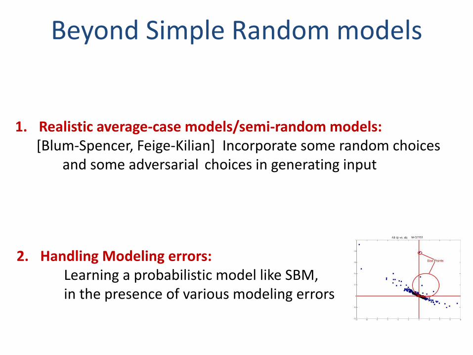
Beyond Simple Random models
1. Realistic average-case models/semi-random models:[Blum-Spencer, Feige-Kilian] Incorporate some random choices
and some adversarial choices in generating input
2. Handling Modeling errors:Learning a probabilistic model like SBM, in the presence of various modeling errors
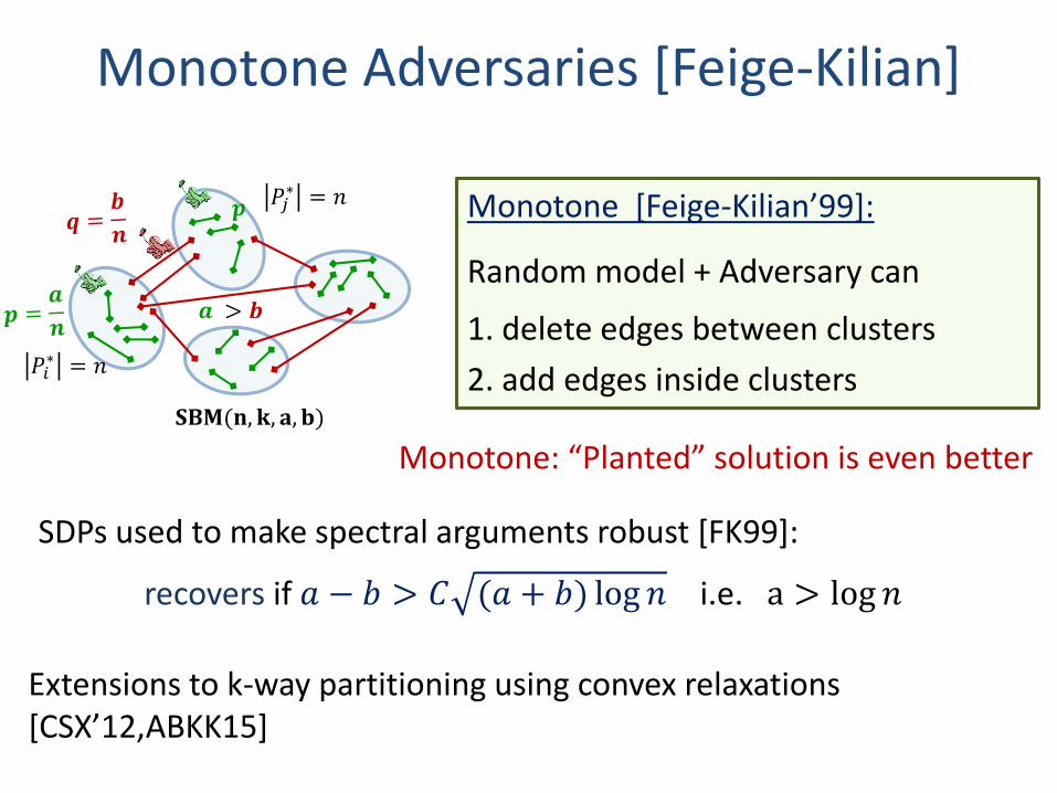
Monotone Adversaries [Feige-Kilian]
Monotone [Feige-Kilian’99]:
Random model + Adversary can
1. delete edges between clusters
2. add edges inside clusters
𝒂 > 𝒃
𝑃𝑖∗ = 𝑛
𝑃𝑗∗ = 𝑛
𝐒𝐁𝐌(𝐧, 𝐤, 𝐚, 𝐛)
Monotone: “Planted” solution is even better
SDPs used to make spectral arguments robust [FK99]:
recovers if 𝑎 − 𝑏 > 𝐶 (𝑎 + 𝑏) log 𝑛 i.e. a > log 𝑛
Extensions to k-way partitioning using convex relaxations [CSX’12,ABKK15]
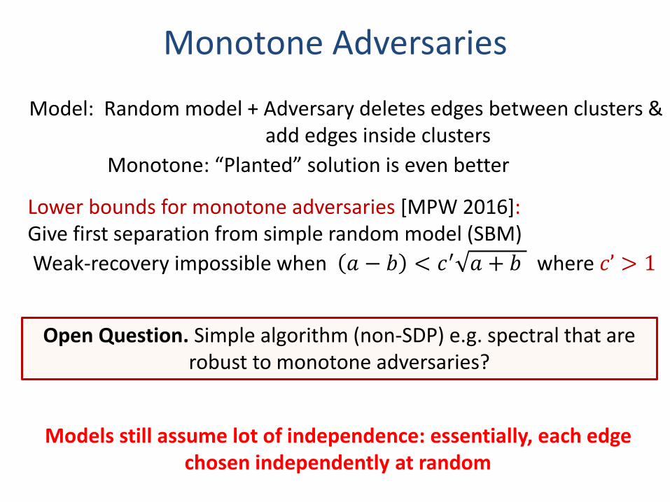
Monotone Adversaries
Model: Random model + Adversary deletes edges between clusters & add edges inside clusters
Models still assume lot of independence: essentially, each edge chosen independently at random
Lower bounds for monotone adversaries [MPW 2016]:Give first separation from simple random model (SBM)
Weak-recovery impossible when 𝑎 − 𝑏 < 𝑐′ 𝑎 + 𝑏 where 𝑐’ > 1
Open Question. Simple algorithm (non-SDP) e.g. spectral that are robust to monotone adversaries?
Monotone: “Planted” solution is even better
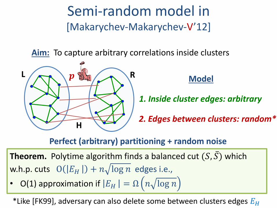
Semi-random model in [Makarychev-Makarychev-V’12]
1. Inside cluster edges: arbitrary
Perfect (arbitrary) partitioning + random noise
RL 𝒑
2. Edges between clusters: random*
Model
Aim: To capture arbitrary correlations inside clusters
*Like [FK99], adversary can also delete some between clusters edges 𝐸𝐻
Theorem. Polytime algorithm finds a balanced cut (𝑆, ҧ𝑆) which
w.h.p. cuts O 𝐸𝐻 + 𝑛 log 𝑛 edges i.e.,
• O(1) approximation if 𝐸𝐻 = Ω 𝑛 log 𝑛
H
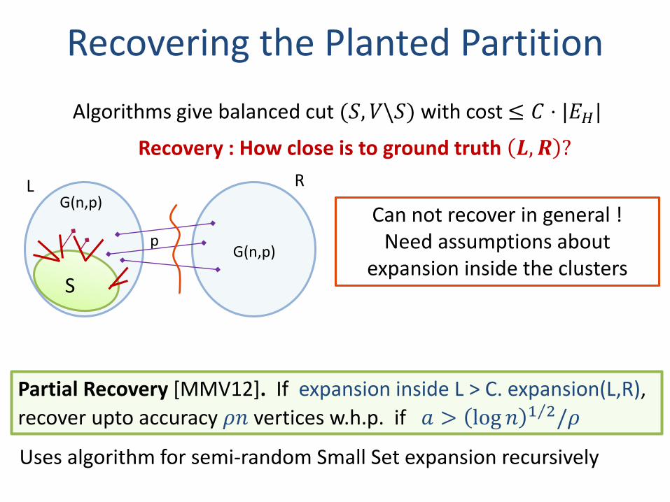
Recovering the Planted Partition
Algorithms give balanced cut (𝑆, 𝑉\𝑆) with cost ≤ 𝐶 ⋅ |𝐸𝐻|
Recovery : How close is to ground truth 𝑳, 𝑹 ?
Can not recover in general !Need assumptions about
expansion inside the clusters
G(n,p)
G(n,p)
L R
S
p
Partial Recovery [MMV12]. If expansion inside L > C. expansion(L,R),
recover upto accuracy 𝜌𝑛 vertices w.h.p. if 𝑎 > log 𝑛 Τ1 2/𝜌
Uses algorithm for semi-random Small Set expansion recursively
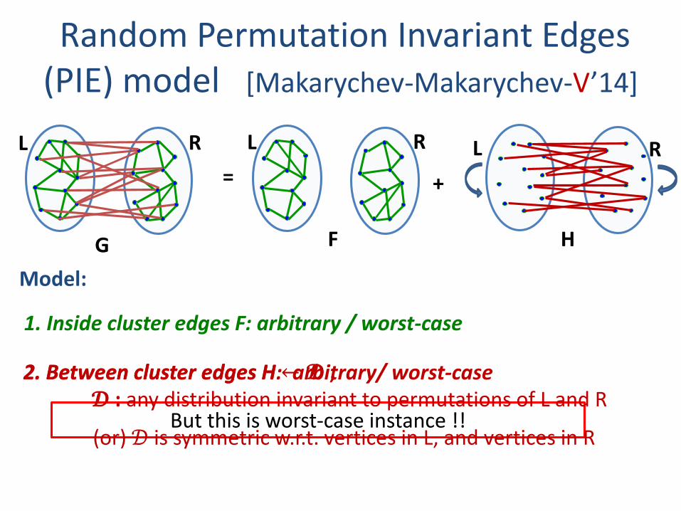
Random Permutation Invariant Edges (PIE) model [Makarychev-Makarychev-V’14]
G H
+=
Model:
1. Inside cluster edges F: arbitrary / worst-case
2. Between cluster edges H: arbitrary/ worst-case
But this is worst-case instance !!
2. Between cluster edges H ← 𝓓 ,𝓓 : any distribution invariant to permutations of L and R
F
RL RLRL
(or) 𝒟 is symmetric w.r.t. vertices in L, and vertices in R
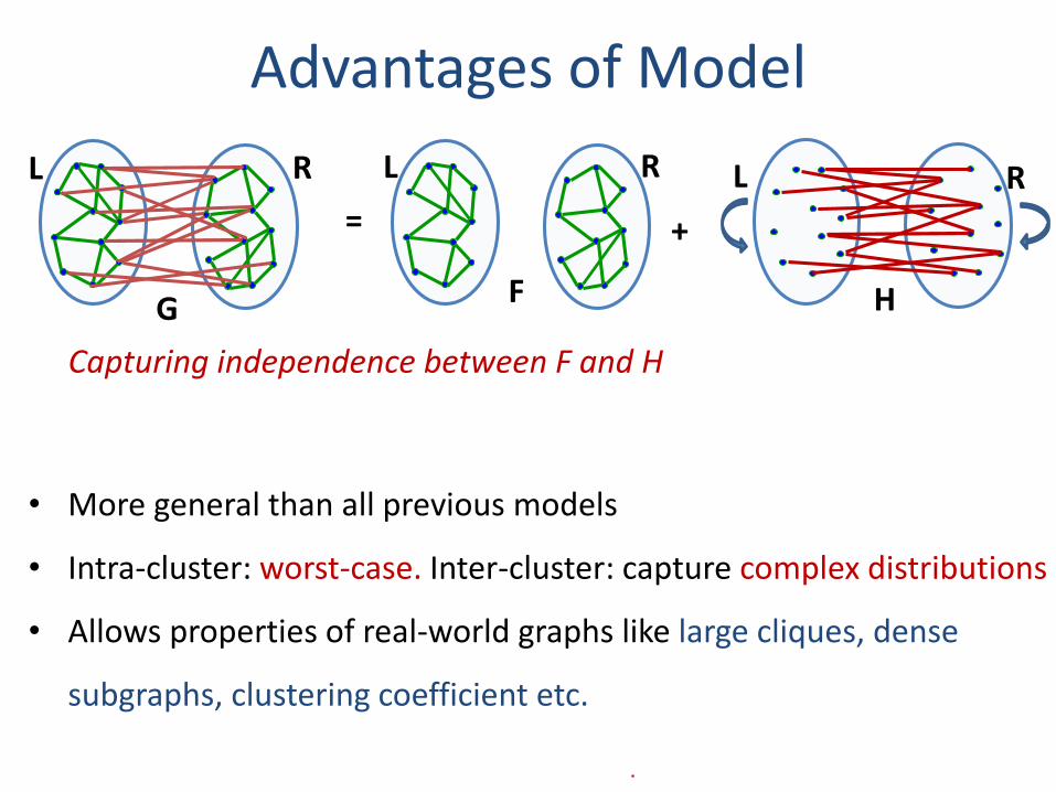
Advantages of Model
H
+=
F
RL RLR
• More general than all previous models
• Intra-cluster: worst-case. Inter-cluster: capture complex distributions
• Allows properties of real-world graphs like large cliques, dense
subgraphs, clustering coefficient etc.
L
Capturing independence between F and H
G
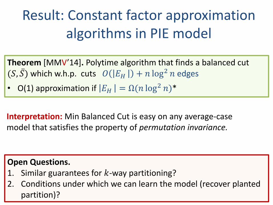
Result: Constant factor approximation algorithms in PIE model
Theorem [MMV’14]. Polytime algorithm that finds a balanced cut (𝑆, ҧ𝑆) which w.h.p. cuts 𝑂 𝐸𝐻 + 𝑛 log2 𝑛 edges
• O(1) approximation if 𝐸𝐻 = Ω(𝑛 log2 𝑛)*
Interpretation: Min Balanced Cut is easy on any average-case model that satisfies the property of permutation invariance.
Open Questions. 1. Similar guarantees for 𝑘-way partitioning?2. Conditions under which we can learn the model (recover planted
partition)?
LEARNING WITH MODELING ERRORS
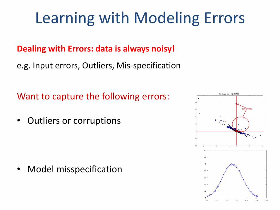
Learning with Modeling Errors
Want to capture the following errors:
• Outliers or corruptions
• Model misspecification
Dealing with Errors: data is always noisy!
e.g. Input errors, Outliers, Mis-specification
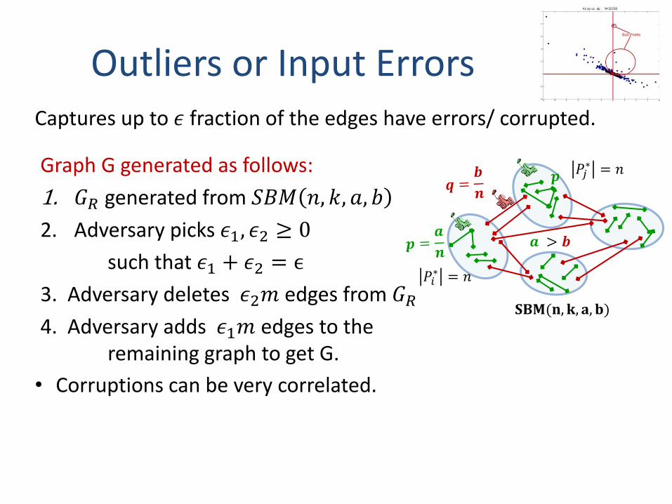
Outliers or Input Errors
𝒂 > 𝒃
𝑃𝑖∗ = 𝑛
𝑃𝑗∗ = 𝑛
𝐒𝐁𝐌(𝐧, 𝐤, 𝐚, 𝐛)
Graph G generated as follows:
1. 𝐺𝑅 generated from 𝑆𝐵𝑀 𝑛, 𝑘, 𝑎, 𝑏
2. Adversary picks 𝜖1, 𝜖2 ≥ 0
such that 𝜖1 + 𝜖2 = ϵ
3. Adversary deletes 𝜖2𝑚 edges from 𝐺𝑅4. Adversary adds 𝜖1𝑚 edges to the
remaining graph to get G.
Captures up to 𝜖 fraction of the edges have errors/ corrupted.
• Corruptions can be very correlated.
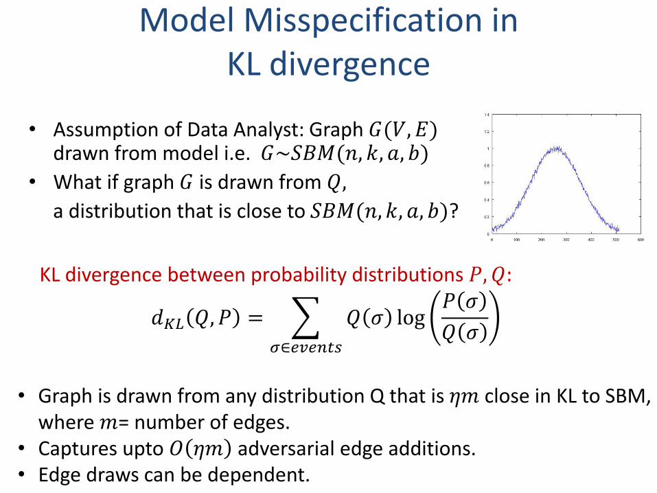
Model Misspecification in KL divergence
• Assumption of Data Analyst: Graph 𝐺(𝑉, 𝐸)drawn from model i.e. 𝐺~𝑆𝐵𝑀(𝑛, 𝑘, 𝑎, 𝑏)
• What if graph 𝐺 is drawn from 𝑄,
a distribution that is close to 𝑆𝐵𝑀(𝑛, 𝑘, 𝑎, 𝑏)?
KL divergence between probability distributions 𝑃, 𝑄:
𝑑𝐾𝐿 𝑄, 𝑃 =
𝜎∈𝑒𝑣𝑒𝑛𝑡𝑠
𝑄 𝜎 log𝑃 𝜎
𝑄 𝜎
• Graph is drawn from any distribution Q that is 𝜂𝑚 close in KL to SBM, where 𝑚= number of edges.
• Captures upto 𝑂 𝜂𝑚 adversarial edge additions.• Edge draws can be dependent.
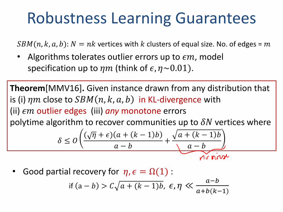
Robustness Learning Guarantees
• Algorithms tolerates outlier errors up to 𝜖𝑚, model specification up to 𝜂𝑚 (think of 𝜖, 𝜂~0.01).
Theorem[MMV16]. Given instance drawn from any distribution that is (i) 𝜂𝑚 close to 𝑆𝐵𝑀 𝑛, 𝑘, 𝑎, 𝑏 in KL-divergence with(ii) 𝜖𝑚 outlier edges (iii) any monotone errorspolytime algorithm to recover communities up to 𝛿𝑁 vertices where
𝛿 ≤ 𝑂( 𝜂 + 𝜖) 𝑎 + 𝑘 − 1 𝑏
𝑎 − 𝑏+
𝑎 + 𝑘 − 1 𝑏
𝑎 − 𝑏
• Good partial recovery for 𝜂, 𝜖 = Ω(1) :
if a − 𝑏 > 𝐶 𝑎 + (𝑘 − 1)𝑏, 𝜖, 𝜂 ≪𝑎−𝑏
𝑎+𝑏(𝑘−1)
𝑆𝐵𝑀(𝑛, 𝑘, 𝑎, 𝑏): 𝑁 = 𝑛𝑘 vertices with 𝑘 clusters of equal size. No. of edges = 𝑚
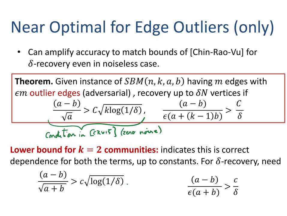
Near Optimal for Edge Outliers (only)
• Can amplify accuracy to match bounds of [Chin-Rao-Vu] for 𝛿-recovery even in noiseless case.
Theorem. Given instance of 𝑆𝐵𝑀 𝑛, 𝑘, 𝑎, 𝑏 having 𝑚 edges with 𝜖𝑚 outlier edges (adversarial) , recovery up to 𝛿𝑁 vertices if
𝑎 − 𝑏
𝑎> 𝐶 𝑘log 1/𝛿 ,
(𝑎 − 𝑏)
𝜖(𝑎 + 𝑘 − 1 𝑏)>
𝐶
𝛿
Lower bound for 𝒌 = 𝟐 communities: indicates this is correct dependence for both the terms, up to constants. For 𝛿-recovery, need
𝑎 − 𝑏
𝑎 + 𝑏> 𝑐 log Τ1 𝛿 𝑎 − 𝑏
𝜖(𝑎 + 𝑏)>𝑐
𝛿
Related Work
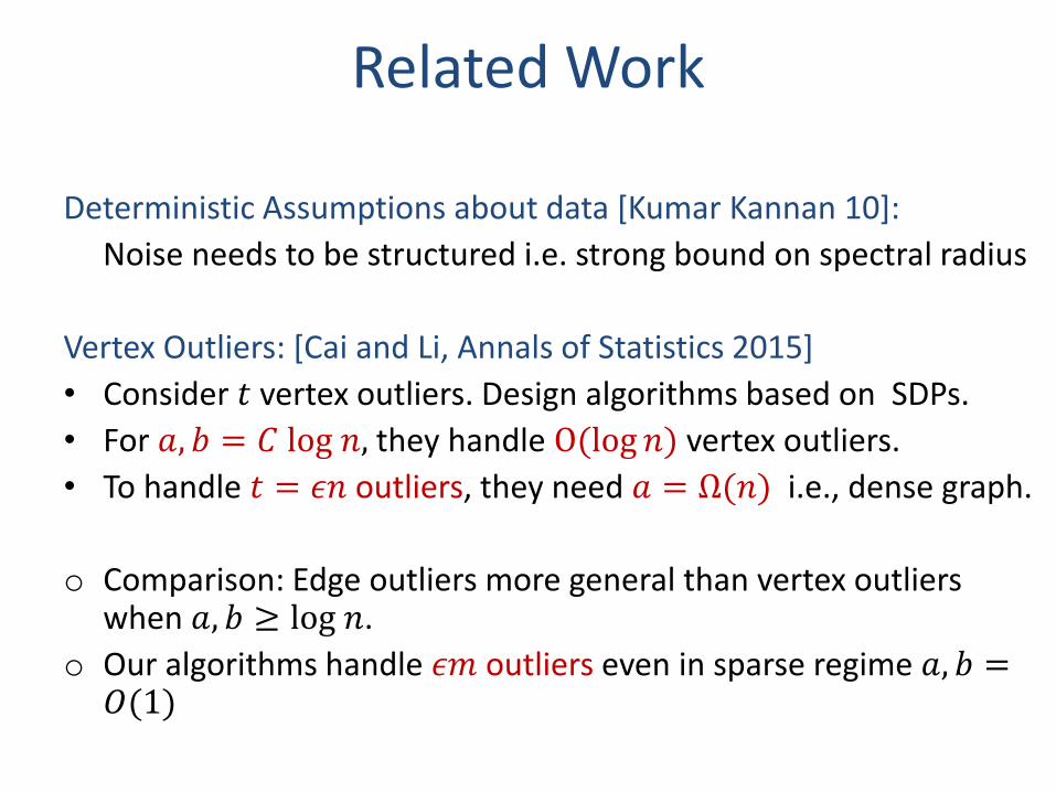
Deterministic Assumptions about data [Kumar Kannan 10]:
Noise needs to be structured i.e. strong bound on spectral radius
Vertex Outliers: [Cai and Li, Annals of Statistics 2015]
• Consider 𝑡 vertex outliers. Design algorithms based on SDPs.
• For 𝑎, 𝑏 = 𝐶 log 𝑛, they handle O(log 𝑛) vertex outliers.
• To handle 𝑡 = 𝜖𝑛 outliers, they need 𝑎 = Ω(𝑛) i.e., dense graph.
o Comparison: Edge outliers more general than vertex outliers when 𝑎, 𝑏 ≥ log 𝑛.
o Our algorithms handle 𝜖𝑚 outliers even in sparse regime 𝑎, 𝑏 =𝑂(1)
ALGORITHM OVERVIEW: LEARNING SBM WITH ERRORS
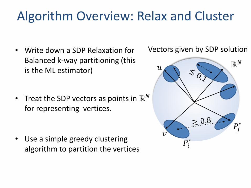
Algorithm Overview: Relax and Cluster
• Write down a SDP Relaxation for Balanced k-way partitioning (this is the ML estimator)
• Treat the SDP vectors as points in ℝ𝑁
for representing vertices.
• Use a simple greedy clustering algorithm to partition the vertices
𝑃𝑖∗
ℝ𝑁
Vectors given by SDP solution
𝑃𝑗∗
𝑢
𝑣
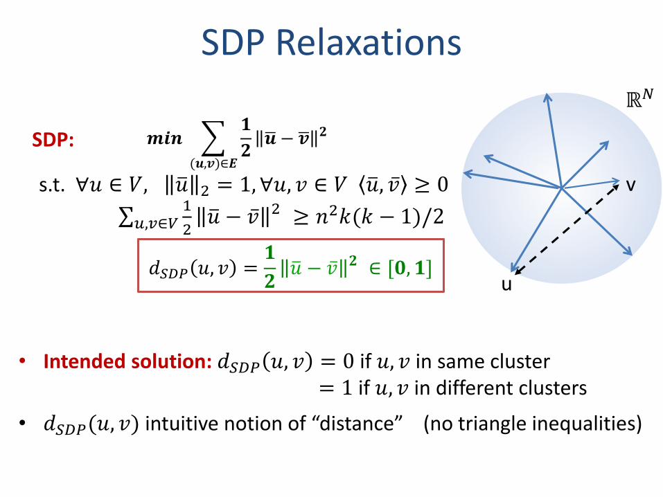
SDP Relaxations
𝒎𝒊𝒏
(𝒖,𝒗)∈𝑬
𝟏
𝟐ഥ𝒖 − ഥ𝒗 𝟐
s.t. ∀𝑢 ∈ 𝑉, ത𝑢 2 = 1, ∀𝑢, 𝑣 ∈ 𝑉 ത𝑢, ҧ𝑣 ≥ 0
σ𝑢,𝑣∈𝑉1
2ത𝑢 − ҧ𝑣 2 ≥ 𝑛2𝑘(𝑘 − 1)/2
SDP:
u
v
ℝ𝑁
• Intended solution: 𝑑𝑆𝐷𝑃 𝑢, 𝑣 = 0 if 𝑢, 𝑣 in same cluster= 1 if 𝑢, 𝑣 in different clusters
• 𝑑𝑆𝐷𝑃(𝑢, 𝑣) intuitive notion of “distance” (no triangle inequalities)
𝑑𝑆𝐷𝑃 𝑢, 𝑣 =𝟏
𝟐ത𝑢 − ҧ𝑣 𝟐 ∈ ሾ𝟎, 𝟏]
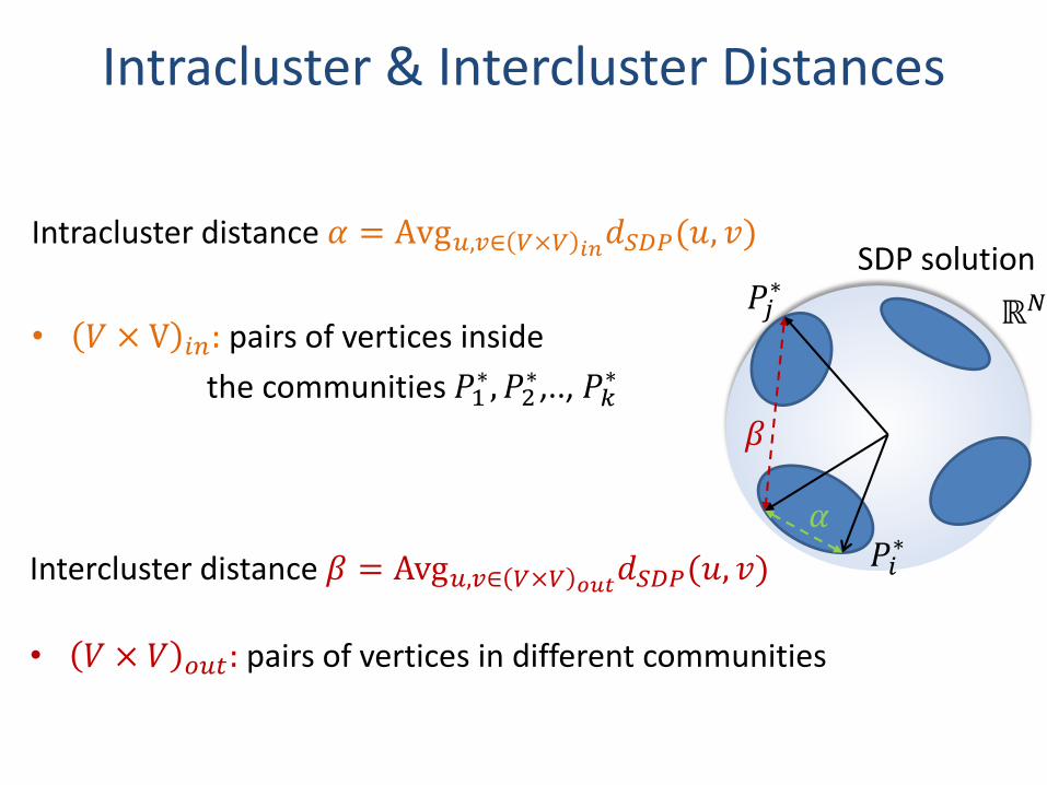
Intracluster & Intercluster Distances
Intracluster distance 𝛼 = Avg𝑢,𝑣∈ 𝑉×𝑉 𝑖𝑛𝑑𝑆𝐷𝑃(𝑢, 𝑣)
• 𝑉 × V 𝑖𝑛: pairs of vertices inside
the communities 𝑃1∗, 𝑃2
∗,.., 𝑃𝑘∗
Intercluster distance 𝛽 = Avg𝑢,𝑣∈ 𝑉×𝑉 𝑜𝑢𝑡𝑑𝑆𝐷𝑃(𝑢, 𝑣)
• 𝑉 × 𝑉 𝑜𝑢𝑡: pairs of vertices in different communities
𝑃𝑖∗
ℝ𝑁
SDP solution𝑃𝑗∗
𝛼
𝛽
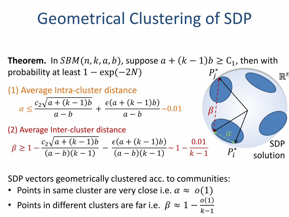
Geometrical Clustering of SDP
Theorem. In 𝑆𝐵𝑀(𝑛, 𝑘, 𝑎, 𝑏), suppose 𝑎 + 𝑘 − 1 𝑏 ≥ C1, then with probability at least 1 − exp(−2𝑁)
(1) Average Intra-cluster distance
𝛼 ≤𝑐2 𝑎 + 𝑘 − 1 𝑏
𝑎 − 𝑏+
𝜖 𝑎 + 𝑘 − 1 𝑏
𝑎 − 𝑏~0.01
(2) Average Inter-cluster distance
𝛽 ≥ 1 −𝑐2 𝑎 + 𝑘 − 1 𝑏
𝑎 − 𝑏 𝑘 − 1−
𝜖 𝑎 + 𝑘 − 1 𝑏
𝑎 − 𝑏 𝑘 − 1~ 1 −
0.01
𝑘 − 1 𝑃𝑖∗
ℝ𝑛
SDP solution
𝑃𝑗∗
𝛼
𝛽
SDP vectors geometrically clustered acc. to communities:• Points in same cluster are very close i.e. 𝛼 ≈ 𝑜(1)
• Points in different clusters are far i.e. 𝛽 ≈ 1 −𝑜 1
𝑘−1
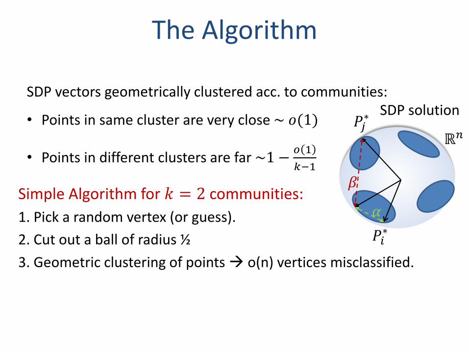
The Algorithm
Simple Algorithm for 𝑘 = 2 communities:
1. Pick a random vertex (or guess).
2. Cut out a ball of radius ½
3. Geometric clustering of points o(n) vertices misclassified.
SDP vectors geometrically clustered acc. to communities:
• Points in same cluster are very close ~ 𝑜(1)
• Points in different clusters are far ~1 −𝑜 1
𝑘−1
𝑃𝑖∗
ℝ𝑛
SDP solution𝑃𝑗∗
𝛼
𝛽
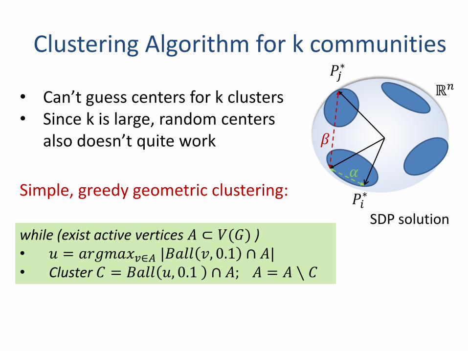
Clustering Algorithm for k communities
while (exist active vertices 𝐴 ⊂ 𝑉(𝐺) )• 𝑢 = 𝑎𝑟𝑔𝑚𝑎𝑥𝑣∈𝐴 |𝐵𝑎𝑙𝑙 𝑣, 0.1 ∩ 𝐴|• Cluster 𝐶 = 𝐵𝑎𝑙𝑙 𝑢, 0.1 ∩ 𝐴; 𝐴 = 𝐴 ∖ 𝐶
Simple, greedy geometric clustering:𝑃𝑖∗
ℝ𝑛
SDP solution
𝑃𝑗∗
𝛼
𝛽
• Can’t guess centers for k clusters• Since k is large, random centers
also doesn’t quite work
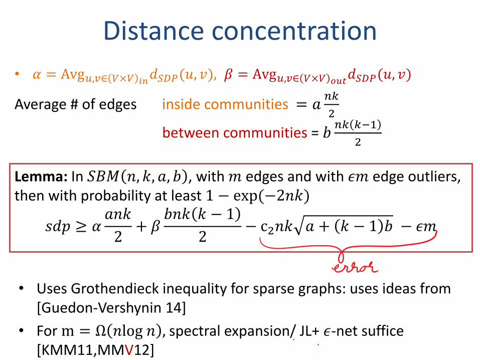
Distance concentration
Lemma: In 𝑆𝐵𝑀 𝑛, 𝑘, 𝑎, 𝑏 , with 𝑚 edges and with 𝜖𝑚 edge outliers, then with probability at least 1 − exp(−2𝑛𝑘)
𝑠𝑑𝑝 ≥ 𝛼𝑎𝑛𝑘
2+ 𝛽
𝑏𝑛𝑘 𝑘 − 1
2− c2𝑛𝑘 𝑎 + 𝑘 − 1 𝑏 − 𝜖𝑚
• 𝛼 = Avg𝑢,𝑣∈ 𝑉×𝑉 𝑖𝑛𝑑𝑆𝐷𝑃(𝑢, 𝑣), 𝛽 = Avg𝑢,𝑣∈ 𝑉×𝑉 𝑜𝑢𝑡
𝑑𝑆𝐷𝑃(𝑢, 𝑣)
Average # of edges inside communities = 𝑎𝑛𝑘
2
between communities = 𝑏𝑛𝑘 𝑘−1
2
• Uses Grothendieck inequality for sparse graphs: uses ideas from [Guedon-Vershynin 14]
• For m = Ω 𝑛log 𝑛 , spectral expansion/ JL+ 𝜖-net suffice [KMM11,MMV12]
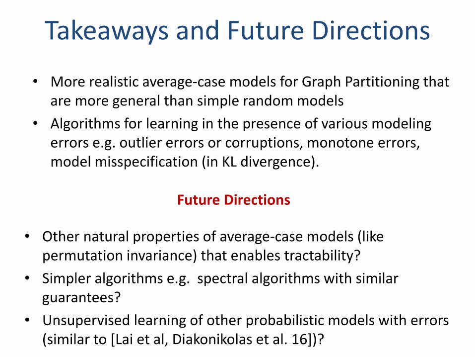
Takeaways and Future Directions
• Other natural properties of average-case models (like permutation invariance) that enables tractability?
• Simpler algorithms e.g. spectral algorithms with similar guarantees?
• Unsupervised learning of other probabilistic models with errors (similar to [Lai et al, Diakonikolas et al. 16])?
Future Directions
• More realistic average-case models for Graph Partitioning that are more general than simple random models
• Algorithms for learning in the presence of various modeling errors e.g. outlier errors or corruptions, monotone errors, model misspecification (in KL divergence).

Thank you!
Questions?
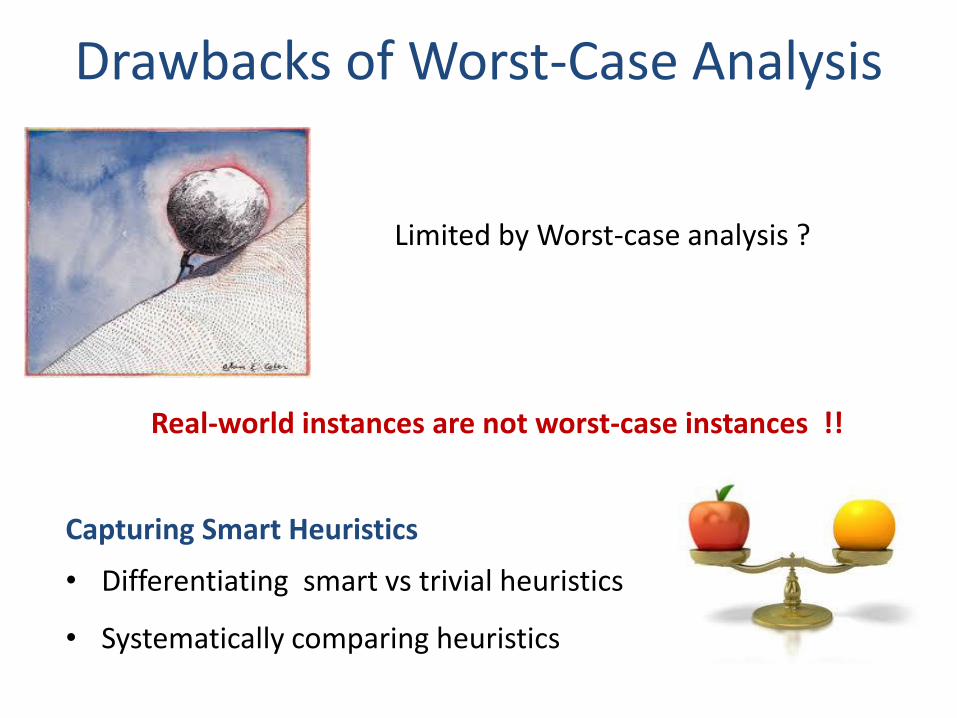
Drawbacks of Worst-Case Analysis
Limited by Worst-case analysis ?
Real-world instances are not worst-case instances !!
Capturing Smart Heuristics
• Differentiating smart vs trivial heuristics
• Systematically comparing heuristics
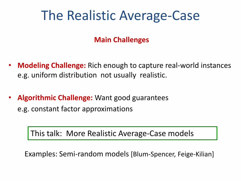
The Realistic Average-Case
Examples: Semi-random models [Blum-Spencer, Feige-Kilian]
Main Challenges
• Modeling Challenge: Rich enough to capture real-world instances e.g. uniform distribution not usually realistic.
• Algorithmic Challenge: Want good guarantees
e.g. constant factor approximations
This talk: More Realistic Average-Case models