Learning Optimal Interventions

Jonas Mueller*, David Reshef, George Du, Tommi Jaakkola

*[email protected]

MIT Computer Science & Artificial Intelligence Laboratory

Dec 10, 2016

Problem Setup

Goal: Identify beneficial interventions from limited (observational) data

Dataset Dn :“ `

xpiq, ypiq˘(n

iid„ PXY

X P Rd = covariates (features) of individual

Y P R = outcome of interest

Objective: Influence X to produce (expected) improvement in Y

(requires simplifying causal assumptions)

Among feasible transformations to X, which one is best?

Limited data ùñ inherent uncertainty regarding Y | X relationship

J. Mueller Dec 10, 2016 2 / 15

Problem Setup

Dataset Dn :“ `

xpiq, ypiq˘(n

iid„ PXY

J. Mueller Dec 10, 2016 2 / 15

Problem Setup

Dataset Dn :“ `

xpiq, ypiq˘(n

iid„ PXY

J. Mueller Dec 10, 2016 2 / 15

Problem Setup

Dataset Dn :“ `

xpiq, ypiq˘(n

iid„ PXY

J. Mueller Dec 10, 2016 2 / 15

Assumptions

(A1) Underlying graphical model: X Ñ rX Ñ Y

X „ PX “ pre-intervention covariate-valuesrX “ values after performing a chosen intervention

(A2) Under no intervention: rX “ X (and in data Dn: rxi “ xi)

(A3) rX “ T pXq (Intervention can be precisely enacted)

T : RdÑ Rd = desired transformation of covariate-values (to guide intervention)

(A4) Y “ fp rXq ` ε (with Erεs “ 0, ε KK rX,X)

J. Mueller Dec 10, 2016 3 / 15

Assumptions

J. Mueller Dec 10, 2016 3 / 15

Assumptions

J. Mueller Dec 10, 2016 3 / 15

Assumptions

Invariant relationship1: Same f for rX produced by any (or no) intervention

1Peters J, Buhlmann P, Meinshausen N. Causal inference using invariant prediction: Identification and confidence intervals.

Journal of the Royal Statistical Society: Series B (2016)

J. Mueller Dec 10, 2016 3 / 15

Overview of Framework

Identifying intervention = find desired transformation policy T

rx “ T pxq P Cx : post-intervention covariate-measurements of individual with initialmeasurements x P Rd, for intervention to enact T , fpT pxqq “ EεrY | rX “ T pxqs

Cx Ă Rd: constraints on possible transformations of x

Cx :“ tz P Rd : |xs´ zs| ď γsu ùñ sth feature cannot be altered by more than γs

Cx :“ tz P Rd : ||x´ z||0 ď ku ùñ at most k features can be intervened upon

J. Mueller Dec 10, 2016 4 / 15

(Step 1) Bayesian inference of posterior f | Dn (eg. Gaussian Process)

Summarized by mean, covariance functions: Erfpxq | Dns, Covprfpxq fpx1qs | Dnq

J. Mueller Dec 10, 2016 4 / 15

(Step 1) Bayesian inference of posterior f | Dn (eg. Gaussian Process)

Summarized by mean, covariance functions: Erfpxq | Dns, Covprfpxq fpx1qs | Dnq

(Step 2) Optimize of T w.r.t. posterior f | Dn (subject to T pxq P Cx)

to identify feasible covariate-transformation likely to improve expected outcomes

(fpT pxqq ą fpxq) according to our current beliefs given limited data

J. Mueller Dec 10, 2016 4 / 15

Personalized Intervention

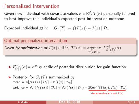
Given new individual with covariate-values x P Rd, T pxq personally tailoredto best improve this individual’s expected post-intervention outcome

Expected individual gain: GxpT q :“ fpT pxqq ´ fpxq | Dn

Optimal personalized intervention

Given by optimization of T pxq P Rd: T ˚pxq “ argmaxT pxqPCx

F´1GxpT qpαq

F´1Gp¨qpαq= αth quantile of posterior distribution for gain function

Posterior for GxpT q summarized bymean = ErfpT pxq | Dns ´ Erfpxq | Dns

variance = VarpfpT pxqq | Dnq ` Varpfpxq | Dnq ´ 2CovpfpT pxqq, fpxq | Dnqloooooooooooooooomoooooooooooooooon

ties uncertainty at x and T pxq

J. Mueller Dec 10, 2016 5 / 15

F´1GxpT qpαq

J. Mueller Dec 10, 2016 5 / 15

F´1GxpT qpαq

J. Mueller Dec 10, 2016 5 / 15

Optimal Personalized Intervention

T ˚pxq improves expected outcome with probability ě 1´ α under ourposterior beliefs (conservatively choose α ă 0.5)

Will never consider T where ErfpT pxq | Dns ă Erfpxq | Dns

Feasible choice T pxq “ x produces objective value of 0

If α is small & uncertainty is high at x (outlier), then T ˚pxq “ x

Philosophy: Doing nothing is greatly preferred to causing harm.

Only propose interventions we are certain will lead to improvement

J. Mueller Dec 10, 2016 6 / 15

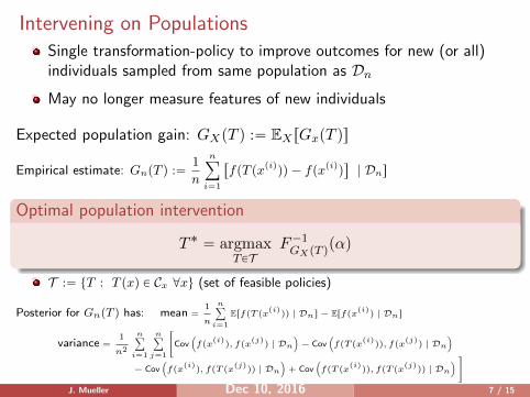
Intervening on PopulationsSingle transformation-policy to improve outcomes for new (or all)individuals sampled from same population as Dn

May no longer measure features of new individuals

Expected population gain: GXpT q :“ EXrGxpT qs

Empirical estimate: GnpT q :“1

fpT pxpiqqq ´ fpxpiqq‰

Optimal population intervention

T ˚ “ argmaxTPT

F´1GXpT qpαq

T :“ tT : T pxq P Cx @xu (set of feasible policies)

Posterior for GnpT q has: mean “1

ErfpT pxpiqqq | Dns ´ Erfpxpiqq | Dns

variance “1

fpxpiqq, fpx

pjqq | Dn

´ Cov´

fpT pxpiqqq, fpx

pjqq | Dn

´ Cov´

fpxpiqq, fpT px

pjqqq | Dn

` Cov´

fpT pxpiqqq, fpT px

pjqqq | Dn

J. Mueller Dec 10, 2016 7 / 15

T ˚ “ argmaxTPT

F´1GXpT qpαq

variance “1

fpxpiqq, fpx

pjqq | Dn

´ Cov´

fpT pxpiqqq, fpx

pjqq | Dn

´ Cov´

fpxpiqq, fpT px

pjqqq | Dn

` Cov´

fpT pxpiqqq, fpT px

pjqqq | Dn

J. Mueller Dec 10, 2016 7 / 15

T ˚ “ argmaxTPT

F´1GXpT qpαq

variance “1

fpxpiqq, fpx

pjqq | Dn

´ Cov´

fpT pxpiqqq, fpx

pjqq | Dn

´ Cov´

fpxpiqq, fpT px

pjqqq | Dn

` Cov´

fpT pxpiqqq, fpT px

pjqqq | Dn

J. Mueller Dec 10, 2016 7 / 15

T ˚ “ argmaxTPT

F´1GXpT qpαq

variance “1

fpxpiqq, fpx

pjqq | Dn

´ Cov´

fpT pxpiqqq, fpx

pjqq | Dn

´ Cov´

fpxpiqq, fpT px

pjqqq | Dn

` Cov´

fpT pxpiqqq, fpT px

pjqqq | Dn

J. Mueller Dec 10, 2016 7 / 15

T ˚ “ argmaxTPT

F´1GXpT qpαq

variance “1

fpxpiqq, fpx

pjqq | Dn

´ Cov´

fpT pxpiqqq, fpx

pjqq | Dn

´ Cov´

fpxpiqq, fpT px

pjqqq | Dn

` Cov´

fpT pxpiqqq, fpT px

pjqqq | Dn

J. Mueller Dec 10, 2016 7 / 15

Types of Global Policy

Form of T cannot depend on x

Sparse intervention: Assume only covariates in chosenintervention-subset I Ă t1, . . . , du are changed(all other covariates remain fixed at their pre-intervention values)

Shift intervention: T pxq “ x`∆∆ P Rd = shift that the policy applies to each individuals’ features(eg. T pxq “ rx1, x2 ` 3, . . . , xds)

Uniform intervention: T pxq “ rz1, . . . , zds where zj “ xj @j R ISets certain covariates to the same constant value for all individuals(eg. T pxq “ rx1, 0, x3, . . . , xds)

J. Mueller Dec 10, 2016 8 / 15

Example: Different Types of Intervention

Contours of outcomes Y expected across feature space rX1, X2s if fpXq “ X1 ¨X2

−2 0 2 4

−4−2

Under sparsity constraint, we must carefully model the underlyingpopulation in order to identify best uniform intervention

J. Mueller Dec 10, 2016 9 / 15

Example: Different Types of Intervention

Contours of outcomes Y expected across feature space rX1, X2s if fpXq “ X1 ¨X2

−2 0 2 4

−4−2

Under sparsity constraint, we must carefully model the underlyingpopulation in order to identify best uniform intervention

J. Mueller Dec 10, 2016 9 / 15

Algorithms

Standard GP prior for f ùñ F´1GpT qpαq has closed form

Smooth kernel ùñ our objectives differentiable w.r.t. T

If altering xs (sth covariate) costs γs per unit, penalize

shift-intervention objective using:dÿ

γs|∆s|

(Use unweighted `1 penalty find sparse shift interventions, γs “ 1)

Employ proximal gradient method for optimization of T

To avoid poor local maxima, use continuation technique

(optimize variants of objective with tapering levels of exaggerated smoothness)

J. Mueller Dec 10, 2016 10 / 15

Algorithms

γs|∆s|

J. Mueller Dec 10, 2016 10 / 15

Algorithms

γs|∆s|

J. Mueller Dec 10, 2016 10 / 15

Algorithms

γs|∆s|

J. Mueller Dec 10, 2016 10 / 15

Summary of Results

Theoretical Guarantee: As nÑ8: maximizer of ourpersonalized/empirical-population intervention-objectives converges tooptimal transformation w.r.t. true f (under reasonable prior)

Theoretical Guarantee: @ n: True f P RKHS of GP prior ùñchosen intervention unlikely to be harmful (probability in terms of α)

GP-based sparse population intervention outperforms standardfrequentist regression methods in gene knockdown application

Beneficial personalized interventions for writing improvement

α “ 0.05 produces far fewer harmful interventions than α “ 0.5

Methods work well in misspecified setting (theory + empirical results)

where sparse-intervention actually affects descendant-covariates in causal DAG

J. Mueller Dec 10, 2016 11 / 15

Summary of Results

Theoretical Guarantee: As nÑ8: maximizer of ourpersonalized/empirical-population intervention-objectives converges tooptimal transformation w.r.t. true f (under reasonable prior)

Theoretical Guarantee: @ n: True f P RKHS of GP prior ùñchosen intervention unlikely to be harmful (probability in terms of α)

GP-based sparse population intervention outperforms standardfrequentist regression methods in gene knockdown application

Beneficial personalized interventions for writing improvement

α “ 0.05 produces far fewer harmful interventions than α “ 0.5

Methods work well in misspecified setting (theory + empirical results)

where sparse-intervention actually affects descendant-covariates in causal DAG

J. Mueller Dec 10, 2016 11 / 15

Population Intervention for Gene Perturbation

X = expression of 10 TF genes2, Y = expression of small moleculemetabolism gene (n “ 161, try 16 different Y )

Propose single TF knockdown (uniform intervention) which will leadto largest down-regulation of metabolism gene

(verification: single gene deletion applied to each TF in subsequent experiments)

ACO1 OPI3 SAM3 MET13 TSL1 GPH1 GSY1 TPS2 GSY2 ZWF1 NTH2 URA7 CAR2 FKS1 PFK27 MGA2

Multivariate Regression Marginal RegressionGP Population Intervention Optimal Intervention

0.8 TSL1

CIN5 -1.5

-0.8 0.6 TSL1

GAT2 -0.8

-0.8 0.4 GPH

(a) (c)(b)

2Kemmeren P et al. Large-scale genetic perturbations reveal regulatory networks and an abundance of gene-specific

repressors. Cell (2014).

J. Mueller Dec 10, 2016 12 / 15

0.8 TSL1

CIN5 -1.5

-0.8 0.6 TSL1

GAT2 -0.8

-0.8 0.4 GPH

(a) (c)(b)

J. Mueller Dec 10, 2016 12 / 15

0.8 TSL1

CIN5 -1.5

-0.8 0.6 TSL1

GAT2 -0.8

-0.8 0.4 GPH

(a) (c)(b)

J. Mueller Dec 10, 2016 12 / 15

Personalized Intervention for Writing Improvement

X = Various text-features3 extracted from articles (eg. word-count,polarity, subjectivity), Y = # of shares on social media (n “ 5000)

Uncertainty-averse method with α “ 0.05 outperforms alternativewhich ignores uncertainty (α “ 0.5), producing half as many harmfulinterventions without reduction in overall average improvement(evaluated in held-out set of new articles)

Proposes different sparse interventions for articles in Businesscategory vs. Entertainment category: Sparse transformations forbusiness articles uniquely advocate decreasing polarity, whereasinterventions to decrease title subjectivity are uniquely prevalent forentertainment articles.

3K Fernandes Vinagre P, Cortez P. A proactive intelligent decision support system for predicting the popularity of online

news. EPIA Portuguese Conference on Artificial Intelligence (2015).

J. Mueller Dec 10, 2016 13 / 15

Misspecified Setting

In practice, sparse interventions may inadvertently affect covariatesdownstream (in causal DAG) of those chosen for intervention(our framework incorrectly assumes T is perfectly enacted)

Find best uniform intervention-policy where T allowed to determinesingle covariate s P t1, . . . , du (T pxq “ rx1, . . . , xs´1, zs, xs`1, . . . , xds)

Intervention actually realized by applying do-operation dopxs “ zsq inunderlying SEM (used to evaluate results)

J. Mueller Dec 10, 2016 14 / 15

Generate data from underlying non-Gaussian linear structuralequation model4

4Shimizu S et al. A linear non-Gaussian acyclic model for causal discovery. JMLR (2006)

J. Mueller Dec 10, 2016 14 / 15

X “ [x1, . . . , x6] , Y “x7SHIMIZU, HOYER, HYVARINEN AND KERMINEN

0.0088

0.54 0.97

-0.063

-0.12 -0.42

0.87 -0.66

-0.019

0.55 0.96

-0.13 -0.43

0.9 -0.68

Figure 4: Left: example original network. Right: estimated network. The sample size was 10000.This shows what kind of mistakes the LiNGAM algorithm might make. The estimatednetwork had one added edge (x1 → x7) and one missing edge (x1 → x6). However, both theadded and missing edges had quite low strengths (x1 → x7, -0.019 and x1 → x6, 0.0088).Note that the other edges were correctly identified, and the connection strengths wereapproximately correct as well.

LiNGAM model. These time windows are then treated as samples of multivariate data. This intro-duces confounding variables to the model, against the assumptions of the LiNGAM analysis. Tosee this, consider an example of an AR(2) process, and a time window of three variables (Figure 5).Here, variables Xt and Xt+1 are confounded by a variable outside the time window. In a generalcase, an AR(p) process introduces confounding variables to p first variables in a time window. TheLiNGAM model holds strictly only for first order processes.

For the tests, a total of 22 data sets were selected from time series data repositories on theInternet (Hyndman, 2005; Statistical Software Information; National Statistics). We did not seekdata sets that would fit the LiNGAM model, but a diverse set of data to see how well the LiNGAManalysis will perform with real-world data, when the assumptions of the model are violated at leastto some extent. The data sets can be roughly categorized as economic time series and environmentaltime series. Economic time series included data sets like currency exchange rates and stock rates.Environmental time series included a more diverse set of data, ranging from monthly river-flows todaily temperatures. Before the tests, the sample autocorrelation and partial autocorrelation functionsfor the series were analyzed to gain insight into how well the series actually fit the AR(p) model.

Sample Size

20 50 100 200 500

−0.5

Sample Size

20 50 100 200 500

Red = uniform intervention selected with GP regression

Blue = best intervention in LinGAM-inferred SEM

J. Mueller Dec 10, 2016 15 / 15

Learning Optimal Interventions

Documents

Transcript of Learning Optimal Interventions