Learning, Expectations Formation, and thePitfalls of Optimal Control Monetary Policy

Athanasios OrphanidesCentral Bank of Cyprus

John C. WilliamsFederal Reserve Bank of San Francisco

Prepared for the FRB Dallas Conference“John Taylor’s Contributions to Monetary Theory and Policy”

October 12–13, 2007

The opinions expressed are those of the authors and do not necessarily reflect the views of the Central Bank of

Cyprus or the management of the Federal Reserve Bank of San Francisco.

Optimal Control Monetary Policy

• Optimal control approach to monetary is back in vogue among academics

(Svensson (2002), Svensson and Woodford (2003), Woodford (2003), Gi-

anonni and Woodford (2005))

• Svensson and Tetlow (2006) show it’s feasible in practice with FRB/US, the

Board’s large-scale nonlinear models

1

Optimal Control Monetary Policy

Optimal control methodology (Sargent, 2007):

1. Apply rational expectations econometrics to historical data to estimate pa-

rameters that describe private agents preferences, technology, endowments,

and information sets.

2. Posit a timing protocol and an objective function for a government, typically

a Pareto criterion.

3. Find a new rational expectations equilibrium that maximizes the governments

objective.

4. Proclaim as advice the government policy that implements that rational ex-

pectations equilibrium.

Source: Thomas J. Sargent (2007), “Evolution and Intelligent Design.”

2

But what if the reference model is misspecified?

• Economists disagree about model specification

• Ironside and Tetlow (2007) show that key properties of the FRB/US model

changed over time reflecting evolution in specification

• Robust control can deal with small deviations from reference model

• But, incorporating “realistic” moderately-sized degree of model uncertainty in

optimal control is infeasible with today’s methods and computers

3

Stress Testing Monetary Policies

• This paper follows the approach of “stress testing” proposed monetary policies

across a range of non-nested empirical macroeconomic models (McCallum

1988; Taylor 1993)

• This approach helps identify characteristics of policy rules that perform well

across different models, and those that don’t

• Past research has identified types of simple monetary policy rules are robust

to misspecification of model dynamics (Levin, Wieland, Williams 1999, 2003;

Orphanides and Williams 2002, 2007)

• Optimal control policies may not be robust to gross misspecifcation of dy-

namics (Levin and Williams 2003)

4

Expectations Formation

•We assume the central bank has the correct model of aggregate dynamics

• But, agents have imperfect knowledge of the macroeconomy and base their

forecasts on estimated models

• Evidence from surveys supports deviations from rational expectations

•We evaluate optimal control policies and simple monetary policy rules op-

timized under the assumption of rational expectations to various models of

learning

5

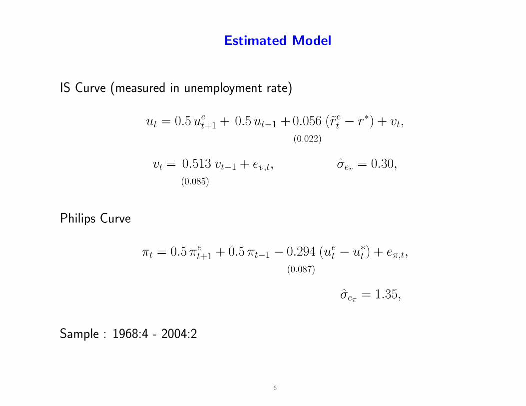
Estimated Model

IS Curve (measured in unemployment rate)

ut = 0.5 uet+1 + 0.5 ut−1 + 0.056

(0.022)

(ret − r∗) + vt,

vt = 0.513(0.085)

vt−1 + ev,t, σev = 0.30,

Philips Curve

πt = 0.5 πet+1 + 0.5 πt−1 − 0.294

(0.087)

(uet − u∗t ) + eπ,t,

σeπ = 1.35,

Sample : 1968:4 - 2004:2

6

Optimal Control Monetary Policy

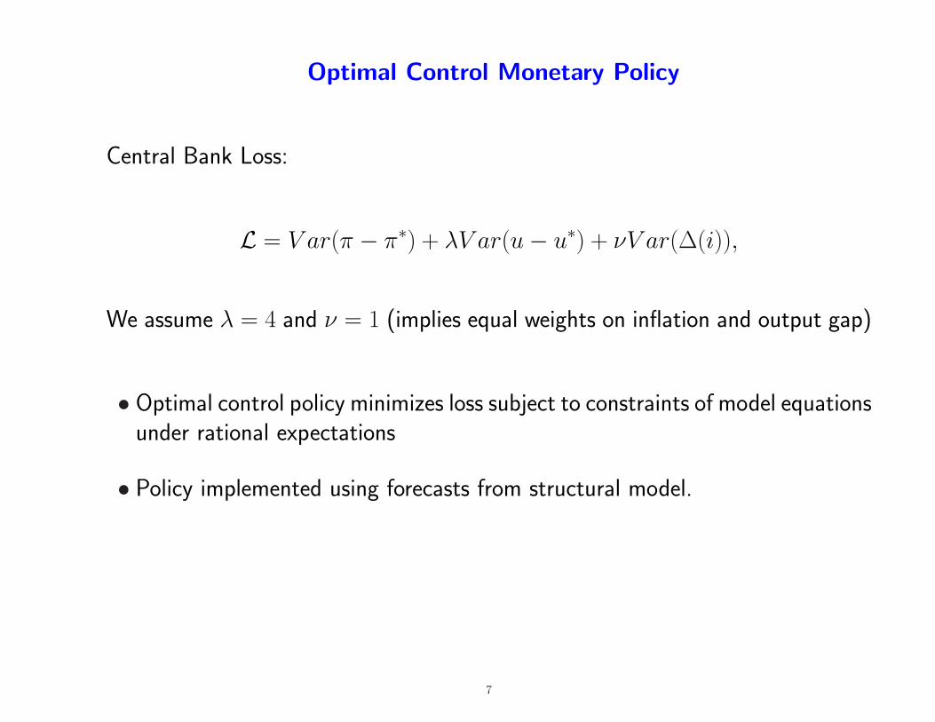
Central Bank Loss:

L = V ar(π − π∗) + λV ar(u− u∗) + νV ar(∆(i)),

We assume λ = 4 and ν = 1 (implies equal weights on inflation and output gap)

• Optimal control policy minimizes loss subject to constraints of model equationsunder rational expectations

• Policy implemented using forecasts from structural model.

7

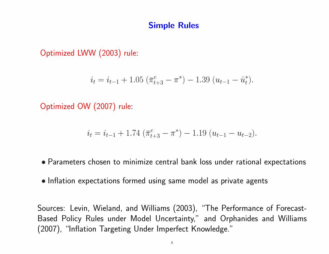
Simple Rules

Optimized LWW (2003) rule:

it = it−1 + 1.05 (πet+3 − π∗)− 1.39 (ut−1 − u∗t ).

Optimized OW (2007) rule:

it = it−1 + 1.74 (πet+3 − π∗)− 1.19 (ut−1 − ut−2).

• Parameters chosen to minimize central bank loss under rational expectations

• Inflation expectations formed using same model as private agents

Sources: Levin, Wieland, and Williams (2003), “The Performance of Forecast-Based Policy Rules under Model Uncertainty,” and Orphanides and Williams(2007), “Inflation Targeting Under Imperfect Knowledge.”

8

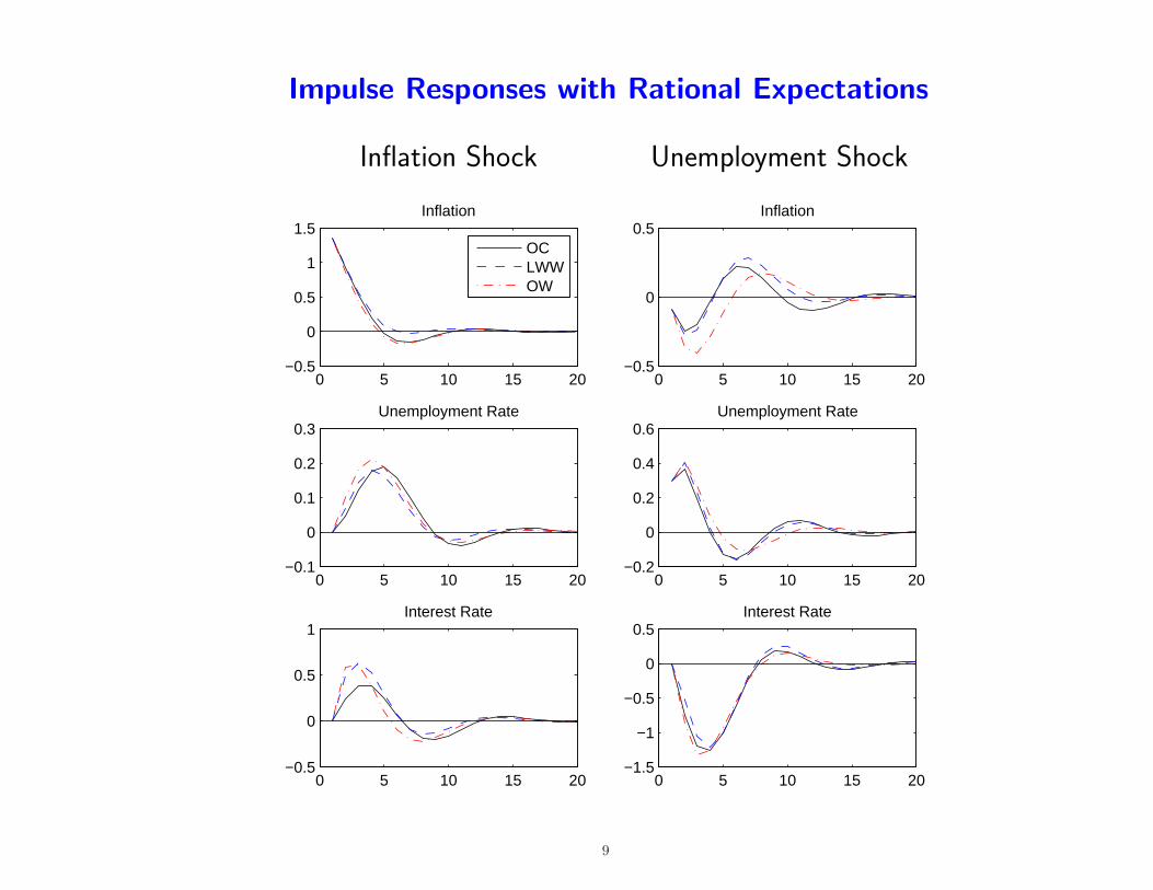
Impulse Responses with Rational Expectations

Inflation Shock Unemployment Shock

0 5 10 15 20−0.5

0

0.5

1

1.5Inflation

OCLWWOW

0 5 10 15 20−0.1

0

0.1

0.2

0.3Unemployment Rate

0 5 10 15 20−0.5

0

0.5

1Interest Rate

0 5 10 15 20−0.5

0

0.5Inflation

0 5 10 15 20−0.2

0

0.2

0.4

0.6Unemployment Rate

0 5 10 15 20−1.5

−1

−0.5

0

0.5Interest Rate

9

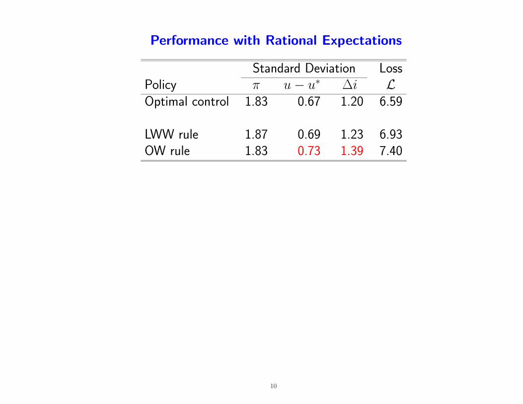
Performance with Rational Expectations

Standard Deviation LossPolicy π u− u∗ ∆i LOptimal control 1.83 0.67 1.20 6.59

LWW rule 1.87 0.69 1.23 6.93OW rule 1.83 0.73 1.39 7.40

10

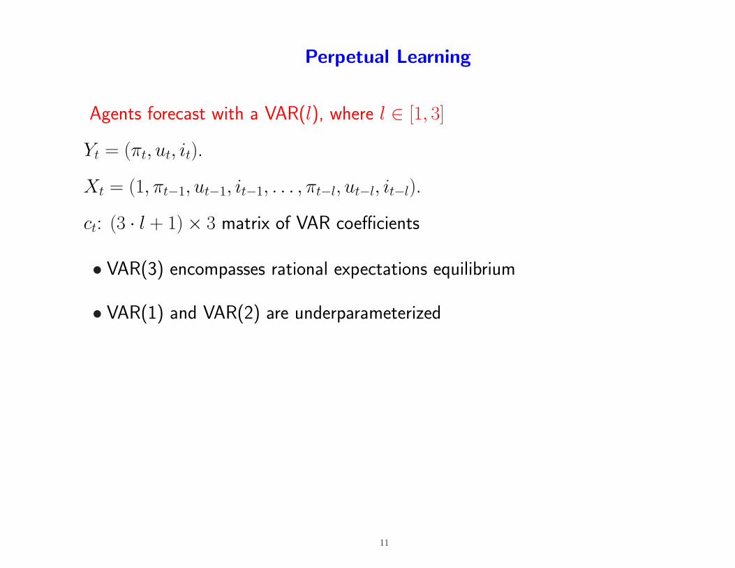
Perpetual Learning

Agents forecast with a VAR(l), where l ∈ [1, 3]

Yt = (πt, ut, it).

Xt = (1, πt−1, ut−1, it−1, . . . , πt−l, ut−l, it−l).

ct: (3 · l + 1)× 3 matrix of VAR coefficients

• VAR(3) encompasses rational expectations equilibrium

• VAR(1) and VAR(2) are underparameterized

11

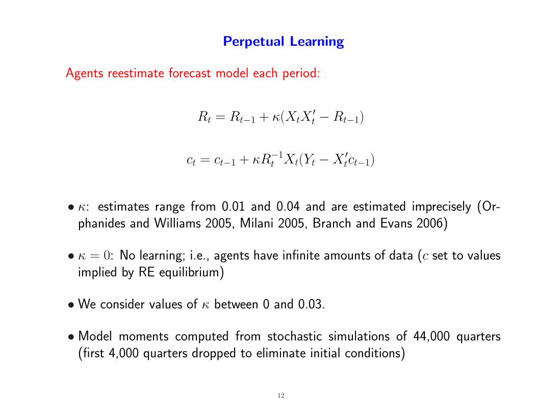
Perpetual Learning

Agents reestimate forecast model each period:

Rt = Rt−1 + κ(XtX′t −Rt−1)

ct = ct−1 + κR−1t Xt(Yt −X ′

tct−1)

• κ: estimates range from 0.01 and 0.04 and are estimated imprecisely (Or-phanides and Williams 2005, Milani 2005, Branch and Evans 2006)

• κ = 0: No learning; i.e., agents have infinite amounts of data (c set to valuesimplied by RE equilibrium)

•We consider values of κ between 0 and 0.03.

•Model moments computed from stochastic simulations of 44,000 quarters(first 4,000 quarters dropped to eliminate initial conditions)

12

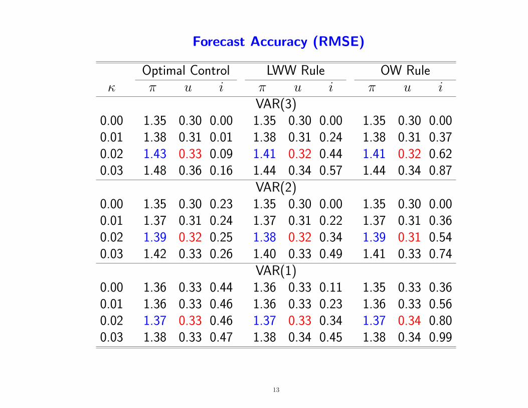
Forecast Accuracy (RMSE)

Optimal Control LWW Rule OW Ruleκ π u i π u i π u i

VAR(3)0.00 1.35 0.30 0.00 1.35 0.30 0.00 1.35 0.30 0.000.01 1.38 0.31 0.01 1.38 0.31 0.24 1.38 0.31 0.370.02 1.43 0.33 0.09 1.41 0.32 0.44 1.41 0.32 0.620.03 1.48 0.36 0.16 1.44 0.34 0.57 1.44 0.34 0.87

VAR(2)0.00 1.35 0.30 0.23 1.35 0.30 0.00 1.35 0.30 0.000.01 1.37 0.31 0.24 1.37 0.31 0.22 1.37 0.31 0.360.02 1.39 0.32 0.25 1.38 0.32 0.34 1.39 0.31 0.540.03 1.42 0.33 0.26 1.40 0.33 0.49 1.41 0.33 0.74

VAR(1)0.00 1.36 0.33 0.44 1.36 0.33 0.11 1.35 0.33 0.360.01 1.36 0.33 0.46 1.36 0.33 0.23 1.36 0.33 0.560.02 1.37 0.33 0.46 1.37 0.33 0.34 1.37 0.34 0.800.03 1.38 0.33 0.47 1.38 0.34 0.45 1.38 0.34 0.99

13

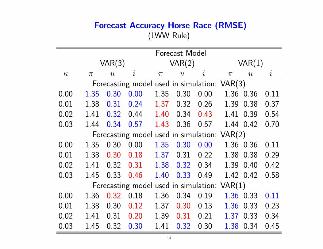
Forecast Accuracy Horse Race (RMSE)(LWW Rule)

Forecast ModelVAR(3) VAR(2) VAR(1)

κ π u i π u i π u iForecasting model used in simulation: VAR(3)

0.00 1.35 0.30 0.00 1.35 0.30 0.00 1.36 0.36 0.110.01 1.38 0.31 0.24 1.37 0.32 0.26 1.39 0.38 0.370.02 1.41 0.32 0.44 1.40 0.34 0.43 1.41 0.39 0.540.03 1.44 0.34 0.57 1.43 0.36 0.57 1.44 0.42 0.70

Forecasting model used in simulation: VAR(2)0.00 1.35 0.30 0.00 1.35 0.30 0.00 1.36 0.36 0.110.01 1.38 0.30 0.18 1.37 0.31 0.22 1.38 0.38 0.290.02 1.41 0.32 0.31 1.38 0.32 0.34 1.39 0.40 0.420.03 1.45 0.33 0.46 1.40 0.33 0.49 1.42 0.42 0.58

Forecasting model used in simulation: VAR(1)0.00 1.36 0.32 0.18 1.36 0.34 0.19 1.36 0.33 0.110.01 1.38 0.30 0.12 1.37 0.30 0.13 1.36 0.33 0.230.02 1.41 0.31 0.20 1.39 0.31 0.21 1.37 0.33 0.340.03 1.45 0.32 0.30 1.41 0.32 0.30 1.38 0.34 0.45

14

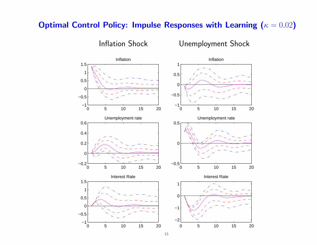
Optimal Control Policy: Impulse Responses with Learning (κ = 0.02)

Inflation Shock Unemployment Shock

0 5 10 15 20−1

−0.5

0

0.5

1

1.5Inflation

0 5 10 15 20−0.2

0

0.2

0.4

0.6Unemployment rate

0 5 10 15 20−1

−0.5

0

0.5

1

1.5Interest Rate

0 5 10 15 20−1

−0.5

0

0.5

1Inflation

0 5 10 15 20−0.5

0

0.5Unemployment rate

0 5 10 15 20−2

−1

0

1

Interest Rate

15

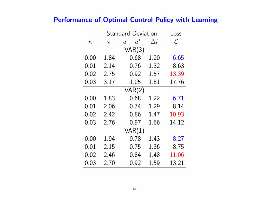
Performance of Optimal Control Policy with Learning

Standard Deviation Lossκ π u− u∗ ∆i L

VAR(3)0.00 1.84 0.68 1.20 6.650.01 2.14 0.76 1.32 8.630.02 2.75 0.92 1.57 13.390.03 3.17 1.05 1.81 17.76

VAR(2)0.00 1.83 0.68 1.22 6.710.01 2.06 0.74 1.29 8.140.02 2.42 0.86 1.47 10.930.03 2.76 0.97 1.66 14.12

VAR(1)0.00 1.94 0.78 1.43 8.270.01 2.15 0.75 1.36 8.750.02 2.46 0.84 1.48 11.060.03 2.70 0.92 1.59 13.21

16

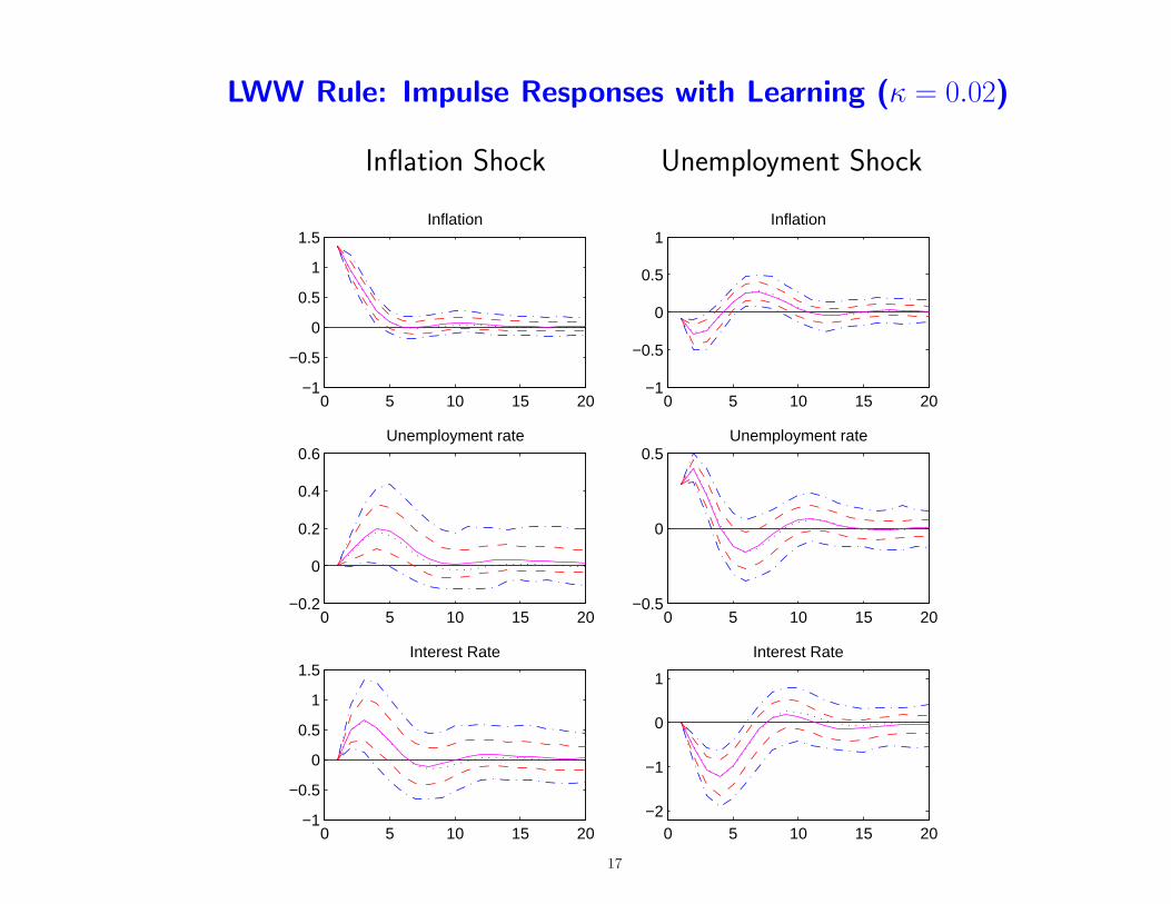
LWW Rule: Impulse Responses with Learning (κ = 0.02)

Inflation Shock Unemployment Shock

0 5 10 15 20−1

−0.5

0

0.5

1

1.5Inflation

0 5 10 15 20−0.2

0

0.2

0.4

0.6Unemployment rate

0 5 10 15 20−1

−0.5

0

0.5

1

1.5Interest Rate

0 5 10 15 20−1

−0.5

0

0.5

1Inflation

0 5 10 15 20−0.5

0

0.5Unemployment rate

0 5 10 15 20−2

−1

0

1

Interest Rate

17

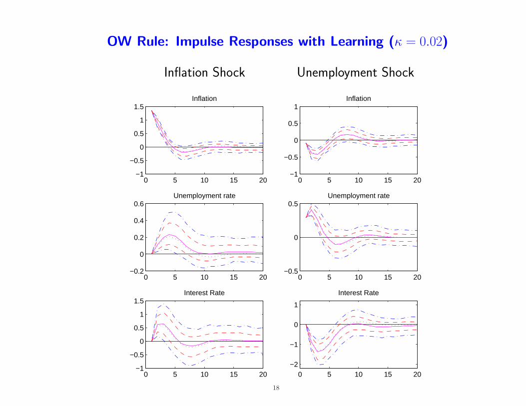
OW Rule: Impulse Responses with Learning (κ = 0.02)

Inflation Shock Unemployment Shock

0 5 10 15 20−1

−0.5

0

0.5

1

1.5Inflation

0 5 10 15 20−0.2

0

0.2

0.4

0.6Unemployment rate

0 5 10 15 20−1

−0.5

0

0.5

1

1.5Interest Rate

0 5 10 15 20−1

−0.5

0

0.5

1Inflation

0 5 10 15 20−0.5

0

0.5Unemployment rate

0 5 10 15 20−2

−1

0

1

Interest Rate

18

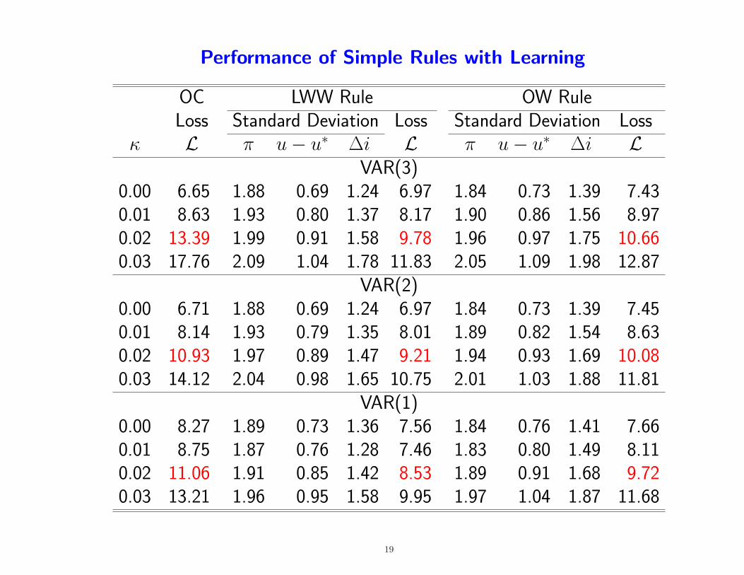
Performance of Simple Rules with Learning

OC LWW Rule OW RuleLoss Standard Deviation Loss Standard Deviation Loss

κ L π u− u∗ ∆i L π u− u∗ ∆i LVAR(3)

0.00 6.65 1.88 0.69 1.24 6.97 1.84 0.73 1.39 7.430.01 8.63 1.93 0.80 1.37 8.17 1.90 0.86 1.56 8.970.02 13.39 1.99 0.91 1.58 9.78 1.96 0.97 1.75 10.660.03 17.76 2.09 1.04 1.78 11.83 2.05 1.09 1.98 12.87

VAR(2)0.00 6.71 1.88 0.69 1.24 6.97 1.84 0.73 1.39 7.450.01 8.14 1.93 0.79 1.35 8.01 1.89 0.82 1.54 8.630.02 10.93 1.97 0.89 1.47 9.21 1.94 0.93 1.69 10.080.03 14.12 2.04 0.98 1.65 10.75 2.01 1.03 1.88 11.81

VAR(1)0.00 8.27 1.89 0.73 1.36 7.56 1.84 0.76 1.41 7.660.01 8.75 1.87 0.76 1.28 7.46 1.83 0.80 1.49 8.110.02 11.06 1.91 0.85 1.42 8.53 1.89 0.91 1.68 9.720.03 13.21 1.96 0.95 1.58 9.95 1.97 1.04 1.87 11.68

19

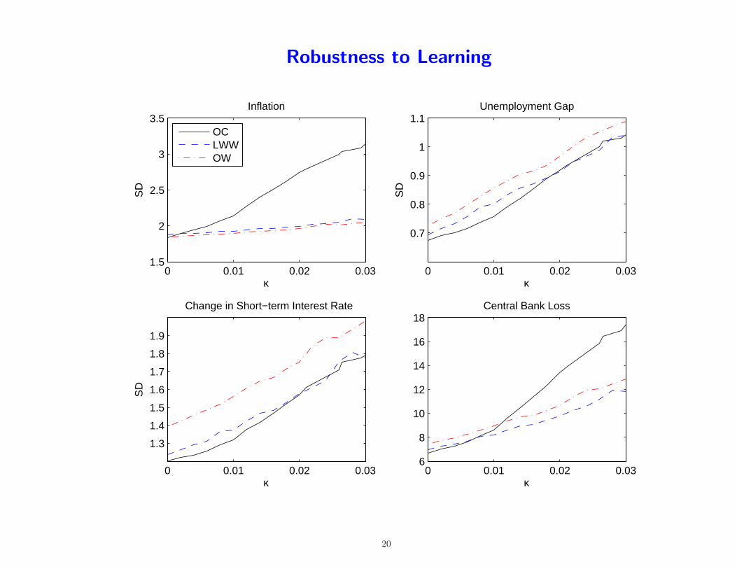
Robustness to Learning

0 0.01 0.02 0.031.5

2

2.5

3

3.5

κ

SD

Inflation

OCLWWOW

0 0.01 0.02 0.03

0.7

0.8

0.9

1

1.1Unemployment Gap

SD

κ

0 0.01 0.02 0.03

1.3

1.4

1.5

1.6

1.7

1.8

1.9

Change in Short−term Interest Rate

SD

κ0 0.01 0.02 0.03

6

8

10

12

14

16

18Central Bank Loss

κ

20

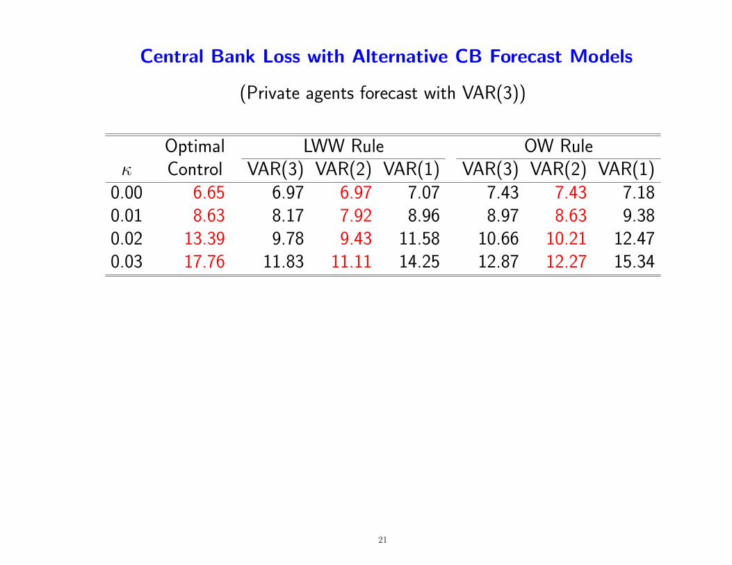
Central Bank Loss with Alternative CB Forecast Models

(Private agents forecast with VAR(3))

Optimal LWW Rule OW Ruleκ Control VAR(3) VAR(2) VAR(1) VAR(3) VAR(2) VAR(1)

0.00 6.65 6.97 6.97 7.07 7.43 7.43 7.180.01 8.63 8.17 7.92 8.96 8.97 8.63 9.380.02 13.39 9.78 9.43 11.58 10.66 10.21 12.470.03 17.76 11.83 11.11 14.25 12.87 12.27 15.34

21

Conclusion and Further Research

• Optimal control policies derived under the assumption of rational expectationsare not robust to alternative models of expectations formation

• Simple rules that have proven to be robust to other forms of model uncertaintyare also robust to alternative models of expectations formation

• Addition of other forms of model misspecification, such as uncertainty abouttime-varying natural rates, amplifies our results (Orphanides and Williams2007)

22