Int J Comput VisDOI 10.1007/s11263-013-0662-8

Learning Discriminative Space–Time Action Parts from WeaklyLabelled Videos

Michael Sapienza · Fabio Cuzzolin ·Philip H.S. Torr

Received: 17 February 2013 / Accepted: 25 September 2013© Springer Science+Business Media New York 2013

Abstract Current state-of-the-art action classificationmethods aggregate space–time features globally, from theentire video clip under consideration. However, the featuresextracted may in part be due to irrelevant scene context,or movements shared amongst multiple action classes. Thismotivates learning with local discriminative parts, whichcan help localise which parts of the video are significant.Exploiting spatio-temporal structure in the video should alsoimprove results, just as deformable part models have provenhighly successful in object recognition. However, whereasobjects have clear boundaries which means we can easilydefine a ground truth for initialisation, 3D space–time actionsare inherently ambiguous and expensive to annotate in largedatasets. Thus, it is desirable to adapt pictorial star models toaction datasets without location annotation, and to featuresinvariant to changes in pose such as bag-of-feature and Fishervectors, rather than low-level HoG. Thus, we propose localdeformable spatial bag-of-features in which local discrimina-tive regions are split into a fixed grid of parts that are allowedto deform in both space and time at test-time. In our experi-mental evaluation we demonstrate that by using local space–

Electronic supplementary material The online version of thisarticle (doi:10.1007/s11263-013-0662-8) contains supplementarymaterial, which is available to authorized users.

M. Sapienza (B)· F. CuzzolinDepartment of Computing and Communication Technologies,Oxford Brookes University, Oxford OX33 1HX, UKe-mail: michael.sapienza-2011@brookes.ac.uk

F. Cuzzoline-mail: fabio.cuzzolin@brookes.ac.uk

P. H.S. TorrDepartment of Engineering Science, University of Oxford,Oxford OX1 3PJ, UKe-mail: philiptorr@hotmail.com

time action parts in a weakly supervised setting, we are ableto achieve state-of-the-art classification performance, whilstbeing able to localise actions even in the most challengingvideo datasets.

Keywords Action classification · Localisation ·Multiple instance learning · Deformable part models ·Space–time videos

1 Introduction

Human action recognition from video is an increasinglyprominent research area in computer vision, with far-reaching applications. On the web, the recognition of humanactions will soon allow the organisation, search, description,and retrieval of information from the massive amounts ofvideo data uploaded each day (Kuehne et al. 2011). In everyday life, human action recognition has the potential to providea natural way to communicate with robots, and novel waysto interact with computer games and virtual environments.

In addition to being subject to the usual nuisance factorssuch as variations in illumination, viewpoint, backgroundand part occlusions, human actions inherently possess a highdegree of geometric and topological variability (Bronstein etal. 2009). Various human motions can carry the exact samemeaning. For example, a jumping motion may vary in height,frequency and style, yet still be the same action. Action recog-nition systems need then to generalise over actions in thesame class, while discriminating between actions of differ-ent classes (Poppe 2010).

Despite these difficulties, significant progress has beenmade in learning and recognising human actions from videos(Poppe 2010; Weinland et al. 2011). Whereas early actionrecognition datasets included videos with single, staged

123

Int J Comput Vis

Fig. 1 The disadvantages of using global information to representaction clips. Firstly, global histograms contain irrelevant backgroundinformation as can be seen in the (a) boxing and (b) running actionvideos of the KTH dataset (Schüldt et al. 2004). Secondly, the his-tograms may contain frequency counts from similar motions occurringin different action classes, such as the (c) trampoline jumping and (d)

volleyball spiking actions in the YouTube dataset (Liu et al. 2009). Inthis paper, we propose a framework in which action models can bederived from local video subvolumes which are more discriminative ofthe action. Thus important differences such as the moving ball, the pres-ence of multiple people and other action-specific characteristics may becaptured

human actions against simple, static backgrounds (Schüldtet al. 2004; Blank et al. 2005), more recently challenginguncontrolled movie data (Laptev et al. 2008) and amateurvideo clips available on the Internet (Liu et al. 2009; Kuehneet al. 2011) have been used to evaluate action recognitionalgorithms. These datasets contain human actions with largevariations in appearance, style, viewpoint, background clut-ter and camera motion, common in the real world.

Current space–time human action classification methods(Jiang et al. 2012; Vig et al. 2012; Kliper-Gross et al. 2012;Wang et al. 2011) derive an action’s representation from anentire video clip, even though this representation may con-tain motion and scene patterns pertaining to multiple actionclasses. For instance, in the state-of-the-art bag-of-feature(BoF) approach (Wang et al. 2009), dense space–time fea-tures are aggregated globally into a single histogram repre-sentation per video. This histogram is generated from fea-tures extracted from the whole video and so includes visualword counts originating from irrelevant scene background(Fig. 1a, b), or from motion patterns shared amongst multi-ple action classes. For example the action classes ‘trampolinejumping’ and ‘volleyball spiking’ from the YouTube dataset(Liu et al. 2009) both involve jumping actions, and have asimilar scene context, as shown in Fig. 1c and d. Thereforein order to discriminate between them, it is desirable to auto-matically select those video parts which tell them apart, suchas the presence of a moving ball, multiple actors and otheraction-specific characteristics.

This motivates a framework in which action models arederived from smaller portions of the video volume, subvol-

umes, which are used as learning primitives rather than theentire space–time video. Thus, we propose to cast action clas-sification in a weakly labelled framework, in which only theglobal label of each video clip is known, and not the label ofeach individual video subvolume. In this way, action mod-els may be derived from automatically selected video partswhich are most discriminative of the action. An exampleillustrating the result of localising discriminative action partswith models learnt from weak annotation is shown in Fig. 2.

In addition to discriminative local action models, we pro-pose to incorporate deformable structure by learning a picto-rial star model for each action class. In the absence of groundtruth location annotation, we use the automatically selectedvideo regions to learn a ‘root’ action model. Action part mod-els are subsequently learnt from the root location after divid-ing it into a fixed grid of regions, which are allowed to deformat test-time. This extends spatial-BoF (SBoF) models (Pariziet al. 2012) to incorporate deformable structure. The resultof testing a 3-part handwaving model is shown in Fig. 3.

The crux of this paper deals with the problem of automati-cally generating action models from weakly labelled observa-tions. By extending global mid-level representations to gen-eral video subvolumes and deformable part-models, we areable to both improve classification results, as compared tothe global baseline, and capture location information.

2 Previous Work

In recent state-of-the-art methods, space–time feature extrac-tion is initially performed in order to convert a video to a

123

Int J Comput Vis

Fig. 2 A handwaving video sequence taken from the KTH dataset(Schüldt et al. 2004) plotted in space and time. Notice that in this par-ticular video, the handwaving motion is repeated continuously and thecamera zoom is varying with time. Overlaid on the video is a densehandwaving-action location map, where each pixel is associated witha score indicating its class-specific saliency. This dense map was gen-

erated by aggregating detection scores from general subvolumes sizes,and is displayed sparsely for clarity, where the colour, from blue to red,and sparsity of the plotted points indicate the action class membershipstrength. Since the scene context of the KTH dataset is not discrimina-tive for this particular action, only the movement in the upper body ofthe actor is detected as salient (best viewed in colour)

Fig. 3 A handwaving video sequence taken from the KTH datasetSchüldt et al. (2004) plotted in space–time. The action is localised inspace and time by a pictorial structure model, despite the latter beingtrained in a weakly supervised framework (in which no action locationannotation is available). Overlaid on the video are the root filter detec-

tions, drawn as red cubes, and part filters (shown in green and bluerespectively), linked to the root by green and blue segments. The starmodel for the handwaving action (above) is detected at multiple stepsin time, and thus well suited to detect actions of unknown duration (bestviewed in colour) (Color figure online)

vectorial representation. Features are extracted around localpoints in each video, which are either determined by a densefixed grid, or by a variety of interest point detectors (IPDs)(Wang et al. 2009). Whereas IPDs such as Harris3D (Laptevand Lindeberg 2003), Cuboid (Dollar et al. 2005) and Hessian(Willems et al. 2008) allow features to be extracted sparsely,saving computational time and memory storage, IPDs are notdesigned to capture smooth motions associated with humanactions, and tend to fire on highlights, shadows, and videoframe boundaries (Gilbert et al 2009; Ke et al. 2010). Further-

more, Wang et al. (2009) demonstrated that dense samplingoutperformed IPDs in real video settings such as the Holly-wood2 dataset (Marszałek et al. 2009), implying that interestpoint detection for action recognition is still an open problem.

A plethora of video features have been proposed todescribe space–time patches, mainly derived from their 2Dcounterparts: Cuboid (Dollar et al. 2005), 3D-SIFT (Scovan-ner et al. 2007), HoG-HoF (Laptev et al. 2008), Local TrinaryPatterns (Yeffet and Wolf 2009) HOG3D (Kläser et al. 2008),extended SURF (Willems et al. 2008), and C2-shape features

123

Int J Comput Vis

(Jhuang et al. 2007). More recently Wang et al. (2011) pro-posed Dense Trajectory features which, when combined withthe standard BoF pipeline (Wang et al. 2009), outperformedthe recent Learned Hierarchical Invariant features (Le et al.2011; Vig et al. 2012). Therefore, even though this frame-work is independent from the choice of features, we usedthe Dense Trajectory features (Wang et al. 2011) to describespace–time video blocks.

Dense Trajectory features are formed by the sequence ofdisplacement vectors in an optical flow field, together withthe HoG-HoF descriptor (Laptev et al. 2008) and the motionboundary histogram (MBH) descriptor (Dalal et al. 2006)computed over a local neighbourhood along the trajectory.The MBH descriptor represents the gradient of the opticalflow, and captures changes in the optical flow field, suppress-ing constant motions (e.g. camera panning) and capturingsalient movements. Thus, Dense Trajectories capture a trajec-tory’s shape, appearance, and motion information. These fea-tures are extracted densely from each video at multiple spatialscales, and a pruning stage eliminates static trajectories suchas those found on homogeneous backgrounds, or spurioustrajectories which may have drifted (Wang et al. 2011).

State-of-the-art results in action classification from chal-lenging human data have recently been achieved by using abag-of-features approach (Jiang et al. 2012; Vig et al. 2012;Kliper-Gross et al. 2012; Wang et al. 2011). Typically, in afirst stage, the local spatio-temporal features are clustered tocreate a visual vocabulary. A query video clip is then rep-resented using the frequency of the occurring visual words,and classification is done using a χ2 kernel support vectormachine (SVM). The surprising success of the BoF methodmay be attributed to its ability to aggregate statistical infor-mation from local features, without regard for the detectionof humans, body-parts or joint locations, which are diffi-cult to robustly detect in unconstrained action videos. How-ever, its representational power initially observed on earlydatasets (Schüldt et al. 2004; Blank et al. 2005) diminishedwith dataset difficulty, e.g. the Hollywood2 dataset (Marsza-łek et al. 2009), and an increasing number of action classes,as in the HMDB51 dataset (Kuehne et al. 2011). This maybe partly due to the fact that current BoF approaches usefeatures from the entire video clips (Wang et al. 2011) orsub-sequences defined in a fixed grid (Laptev et al. 2008),without considering the location of the action. Thus, manysimilar action parts and background noise also contribute tothe global histogram representation.

Recent work by Vig et al. (2012) used saliency modelsto prune features and build discriminative histograms forthe Hollywood2 action classification dataset (Marszałek etal. 2009). Amongst various automatic approaches to esti-mate action saliency, such as tensor decomposition, the bestapproach selected features according to their spatial distanceto the video centre; a central mask. This approach is ideal for

Hollywood movies in which actors are often centred by thecameraman, but less well suited for general videos captured‘in the wild’. Furthermore, the saliency masks were precom-puted for each video individually, without considering thedataset’s context. For example, in a dataset of general sportsactions, the presence of a swimming pool is highly discrimi-native of the action diving. Less so in a dataset which containsonly different types of diving action categories. Thus, in ourview, action saliency should also depend on the differencesbetween actions in distinct classes.

Attempts to incorporate action structure into the BoFrepresentation for video classification have been based onthe spatial pyramid approach (Laptev et al. 2008); here aspatio-temporal grid was tuned for each dataset and actionclass. Although spatial pyramids have been successful inscene classification (Lazebnik et al. 2006), in which partsof the scene consistently appear in the same relative loca-tions across images, it is unclear whether they are useful fordifficult clips such as those captured from mobile devices,in which the same action can appear in any location of thevideo.

In order to model human actions at a finer scale, it isdesirable to localise the spatial and temporal extent of anaction. Initial work by Laptev and Pérez (2007) learnt aboosted cascade of classifiers from spatio-temporal features.To improve space–time interest point detectors for actionssuch as ‘drinking’, the authors incorporated single framedetection from state-of-the-art methods in object detection. Itis however desirable to remove the laborious and ambiguoustask of annotating keyframes, especially when consideringhuge online video datasets.

In another approach, Kläser et al. (2010) split the task intotwo: firstly by detecting and tracking humans to determinethe action location in space, and secondly by using a space–time descriptor and sliding window classifier to temporallylocate two actions (phoning, standing up). In a similar spirit,our goal is to localise actions in space and time, rather thantime alone (Duchenne et al. 2009; Gaidon et al. 2011). How-ever, instead of resorting to detecting humans in every frameusing a sliding window approach (Kläser et al. 2010), welocalise actions directly in space–time, either by aggregatingdetection scores (Fig. 2), or by visualising the 3D boundingbox detection windows (Fig. 3).

To introduce temporal structure into the BoF framework,Gaidon et al. (2011) introduced Actom Sequence Mod-els, based on a non-parametric generative model. In videoevent detection, Ke et al. (2010) used a search strategyin which oversegmented space–time video regions werematched to manually constructed volumetric action tem-plates. Inspired by the pictorial structures framework (Fis-chler and Elschlager 1973), which has been successful atmodelling object part deformations (Felzenszwalb et al.2010), Ke et al. (2010) split their action templates into

123

Int J Comput Vis

deformable parts making them more robust to spatial andtemporal action variability. Despite these efforts, the actionlocalisation techniques described (Laptev and Pérez 2007;Kläser et al. 2010; Ke et al. 2010) require manual labellingof the spatial and/or temporal (Gaidon et al. 2011) extentof the actions/parts in a training set. In contrast, we pro-pose to learn discriminative action models automaticallyfrom weakly labelled observations, without human locationannotation. Moreover, unlike previous work (Gilbert et al2009; Liu et al. 2009), we select local discriminative sub-volumes represented by mid-level features (Boureau et al.2010) such as BoF and Fisher vectors, and not the low-levelspace–time features themselves (e.g. HoG, HoF). Since inaction clip classification only the class of each action clipas a whole is known, and not the class labels of individ-ual subvolumes, this problem is inherently weakly-labelled.We therefore cast video subvolumes and associated repre-sentations as instances in a discriminative multiple instancelearning (MIL) framework.

Some insight into MIL comes from its use in the contextof face detection (Viola et al. 2005). Despite the availabil-ity of ground truth bounding box annotation, the improve-ment in detection results when compared to those of afully supervised framework suggested that there existed amore discriminative set of ground truth bounding boxes thanthose labelled by human observers. The difficulty in man-ual labelling arises from the inherent ambiguity in labellingobjects or actions (bounding box scale, position) and judg-ing, for each image/video, whether the context is importantfor that particular example or not. A similar MIL approachwas employed by Felzenszwalb et al. (2010) for object detec-tion in which possible bounding box locations were cast aslatent variables. This allowed the self-adjustment of the pos-itive ground truth data, better aligning the learnt object filtersduring training.

In order to incorporate object structure, Felzenszwalb etal. (2010) used a star-structured part-based model, definedby a ‘root’ filter, a set of ‘parts’, and a structure model. How-ever, the objects considered had a clear boundary which wasannotated by ground truth bounding boxes. During training,the ground truth boxes were critical for finding a good ini-tialisation of the object model, and also constrained the plau-sible position of object parts. Furthermore, the aspect ratioof the bounding box was indicative of the viewpoint is wasimaged from, and was used to split each object class into amixture of models (Felzenszwalb et al. 2010). In contrast,for action classification datasets such as the ones used inthis work, the spatial location, the temporal duration andthe number of action instances are not known beforehand.Therefore we propose an alternative approach in which partmodels are learnt by splitting the ‘root’ filter into a gridof fixed regions, as done in spatial pyramids (Lazebnik etal. 2006; Parizi et al. 2012). In contrast to the rigid global

grid regions of spatial pyramids (Lazebnik et al. 2006) orSBoF (Parizi et al. 2012), our rigid template used duringtraining is local, not global, and is allowed to deform attest-time to better capture the action warping in space andtime.

At test time, human action classification is achieved bythe recognition of action instances in the query video, afterdevising a sensible mapping from instance scores to thefinal clip classification decision. To this end, we use mul-tiple instance learning (MIL), in which the recovery of boththe instance labels and bag labels is desired, without usingtwo separate iterative algorithms (Andrews et al. 2003).Our proposed SVM-map strategy provides a mapping frominstance scores to bag-scores which quantitatively outper-forms taking the argument of the maximum score in eachbag.

An early version of this work appeared in Sapienza et al.(2012), and has been extended to include general subvolumeshapes rather than fixed size cubes (Sapienza et al. 2012),deformable part models, efficient methods to handle the largescale nature of the problem, and an extended experimentalevaluation.

The contributions of this work are as follows:

– (i) We cast the conventionally supervised BoF action clas-sification approach into a weakly supervised setting andlearn action models and discriminative video parts simul-taneously via MIL.

– (ii) We propose adding deformable structure to localmid-level action representations (e.g. BoF, Fisher). Thisextends SBoF to allow the deformation of the rigid tem-plate at test-time.

– (iii) We demonstrate that our SVM-map strategy for map-ping instance scores to global clip classification scoresoutperforms taking the argument of the maximum instancescore in each video.

– (iv) Finally we show qualitative localisation results usinga combination of classification and detection to outputaction-specific saliency maps; we are the first to showqualitative localisation results on challenging movie datasuch as the HMDB51 dataset.

3 Methodology

The proposed action recognition system is composed ofthree main building blocks: (i) learning discriminative localaction subvolumes (Sect. 3.1), (ii) learning and matchingof part models extracted from the learnt ‘root’ subvolumes(Sect. 3.2), and (iii) mapping local instance scores appro-priately to global video clip scores (Sect. 3.3). The sec-tions which follow are presented as extensions to BoF;however the same methodology extends to other mid-

123

Int J Comput Vis

level feature representations, as shown in the experiments(Sect. 4).

3.1 MIL-BoF Action Models

In this work, when using BoF, we define an instance to bean individual histogram obtained by aggregating the DenseTrajectory features within a local subvolume, and a bag isdefined as a set of instances originating from a single space–time video. Since we perform multi-class classification witha one-vs-all approach, we present the following methodologyas a binary classification problem.

In action classification datasets, each video clip is assignedto a single action class label. By decomposing each videointo multiple instances, now only the class of the originatingvideo is known and not those of the individual instances.This makes the classification task weakly labelled, where itis known that positive examples of the action exist within thevideo clip, but their exact location is unknown. If the labelof the bag is positive, then it is assumed that one or moreinstances in the bag will also be positive. If the bag has anegative label, then all the instances in the bag must retain anegative label. The task here is to learn the class membershipof each instance, and an action model to represent each class,as illustrated in Fig. 4.

The learning task may be cast in a max-margin multipleinstance learning framework, of which the pattern/instancemargin formulation (Andrews et al. 2003) is best suited forspace–time action localisation. Let the training set D =(〈X1, Y1〉, . . . , 〈Xn, Yn〉) consist of a set of bags Xi ={xi1, . . . , ximi } of different length mi , with correspondingground truth labels Yi ∈ {−1,+1}. Each instance xi j ∈ R

represents the j th BoF model in the i th bag, and has an asso-ciated latent class label yi j ∈ {−1,+1} which is initially

unknown for the positive bags (Yi = +1). The class labelfor each bag Yi is positive if there exists at least one positiveinstance in the bag, that is, Yi = max j {yi j }. Therefore thetask of the mi-MIL is to recover the latent class variable yi j

of every instance in the positive bags, and to simultaneouslylearn an SVM instance model 〈w, b〉 to represent each actionclass.

The max-margin mi-SVM learning problem results in asemi-convex optimisation problem, for which Andrews etal. (2003) proposed a heuristic approach. In mi-SVM, eachinstance label is unobserved, and we maximise the usual soft-margin jointly over hidden variables and discriminant func-tion:

minyij

minw,b,ξ

1

2‖w‖2 + C

∑

ij

ξij, (1)

subject to : yi j (wT xi j + b) ≥ 1 − ξi j , ∀i, j

yi j ∈ {−1,+1}, ξi j ≥ 0,

and∑

j∈i

(1 + yi j )/2 ≥ 1 s.t. Yi = +1,

yi j = −1 ∀ j∈i s.t. Yi = −1,

where w is the normal to the separating hyperplane, b is theoffset, and ξi j are slack variables for each instance xi j .

The heuristic algorithm proposed by Andrews et al. (2003)to solve the resulting mixed integer problem is laid out inAlgorithm 1. Consider training a classifier for a walking classaction from the bags of training instances in a video dataset.Initially all the instances are assumed to have the class labelof their parent bag/video (STEP 1). Next, a walking actionmodel estimate 〈w, b〉 is found using the imputed labels yi j

(STEP 2), and scores

Fig. 4 Instead of defining an action as a space–time pattern in an entirevideo clip (a), an action is defined as a collection of space–time actionparts contained in general subvolumes shapes of cube/cuboidial shape(b). One ground-truth action label is assigned to the entire space–time

video or ‘bag’, while the labels of each action subvolume or ‘instance’are initially unknown. Multiple instance learning is used to learn whichinstances are particularly discriminative of the action (solid-line cubes),and which are not (dotted-line cubes)

123

Int J Comput Vis

Algorithm 1 Heuristic algorithm proposed by (Andrews etal, 2003) for solving mi-SVM.

STEP 1. Assign positive labels to instances in positive bags: yi j = Yifor j ∈ irepeat

STEP 2. Compute SVM solution 〈w, b〉 for instances with estimatedlabels yi j .STEP 3. Compute scores fi j = wT xi j + b for all xi j in positivebags.STEP 4. Set yi j = sgn( fi j ) for all j ∈ i , Yi = 1.for all positive bags Xi do

if∑

j∈i (1 + yi j )/2 == 0 then

STEP 5. Find j∗ = argmaxj∈i

fi j , set y∗i j = +1

end ifend for

until class labels do not changeOutput w, b

fi j = wT xi j + b, (2)

for each instance in the bag are estimated with the currentmodel (STEP 3). Whilst the negative labels remain strictlynegative, the positive labels may retain their current label, orswitch to a negative label (STEP 4). If, however, all instancesin a positive bag become negative, then the least negativeinstance in the bag is set to have a positive label (STEP 5),thus ensuring that there exists at least one positive examplein each positive bag.

Now consider walking video instances whose feature dis-tribution is similar to those originating from bags in distinctaction classes. The video instances originating from the walk-ing videos will have a positive label, whilst those from theother action classes will have a negative label (assuming a1-vs-all classification approach). This corresponds to a sit-uation where points in the high dimensional instance spaceare near to each other. Thus, when these positive walkinginstances are reclassified in a future iteration, it is likely thattheir class label will switch to negative. As the class labels areupdated in an iterative process, eventually only the discrimi-native instances in each positive bag are retained as positive.The resulting SVM model 〈w0, b0〉 represents the root filterin our space–time BoF star model.

3.2 Local Deformable SBoF Models (LDSBoF)

In order to learn space–time part models, we first select thebest scoring root subvolumes learnt via Algorithm 1. Theselection is performed by first pruning overlapping detectionswith non-maximum suppression in space and time, and thenpicking the top scoring 5 %. Subvolumes are considered tobe overlapping if their intersection over the union is greaterthat 20 %. This has the effect of generating a more diversesample of high scoring root subvolumes to learn the partmodels from.

(a)

(b)

Fig. 5 Action recognition with a local deformable spatial bag-of-features model (LDSBoF). (a) Training ‘root’ and ‘part’ action models.The method described in Sect. 3.1 first selects discriminative root sub-volumes (red cube). To learn part filters, the ‘root’ subvolume is dividedinto a grid of parts; in this case a temporal grid with two parts as denotedby the red dotted line. (b) At test time, the root filter alone (solid redcube) learnt from the action in (a) is not suited to detect the action in(b). However, it is better able to detect this type of action variation withthe addition of part filters (solid green and blue cuboids) loosely con-nected to the root. (a) A training action sequence of class jumping. Adiscriminative local action subvolume selected via MIL is drawn as ared solid-line cube. The dotted red line denotes the temporal grid intowhich the root is split in order to learn two separate part models. (b) Atest action sequence of class ‘jumping’ similar to that in (a) but stretchedin time. The detected ‘root’ subvolume is drawn as a red solid cube, andthe parts are shown as green and blue cuboids respectively (Color figureonline)

The part models are generated by splitting the root sub-volumes using a fixed grid, as illustrated in Fig. 5a and b.For our experiments we split the root into p = 2 equal-sized blocks along the time dimension Fig. 5a, and recal-culate BoF vectors for each part. We found that with ourcurrent dense low-level feature sampling density (Sect. 4.2),further subdividing the root to generate more parts createssubvolumes which are too small to aggregate meaningfulstatistics. Finally, part models 〈wk, bk〉, k = {1, . . . , p},are individually learnt using a standard linear SVM. Thegrid structure of SBoF removes the need to learn a struc-ture model for each action class, which simplifies training,especially since no exact or approximate location annotationis available to constrain the part positions (Felzenszwalb etal. 2010).

In the following, an action is defined in terms of a col-lection of space–time action-parts in a pictorial structuremodel (Fischler and Elschlager 1973; Felzenszwalb and Hut-tenlocher 2005; Ke et al. 2010), as illustrated in Fig. 5b. Let

123

Int J Comput Vis

an action be represented by an undirected graph G = (V, E),where the vertices V = {v1, . . . , vp} represent the p parts ofthe action, and E is a set of edges such that an edge ekl repre-sents a connection between part vk and vl . An instance of theaction’s configuration is defined by a vector L = (l1, . . . , l p),where lk ∈ R

3 specifies the location of part vk . The detectionspace S(x, y, t) is represented by a feature map H of BoFhistograms for each subvolume at position lk , and there existsfor each action part, a BoF filter wk , which when correlatedwith a subvolume in H, gives a score indicating the presenceof the action part vk . Thus, the dot product

wk · φ(H, lk), (3)

measures the correlation between a filter wk and a featuremap H at location lk in the video. Let the distance betweenaction parts dkl(lk, ll) be a cost function measuring the degreeof deformation of connected parts from a model. The overallscore for an action located at root position l0 is calculated as:

si j (l0) = maxl1,...l p

( p∑

k=0

wk · φ(Hi , lk) −p∑

k=1

dkl(lk, ll)

), (4)

which optimises the appearance and configuration of theaction parts simultaneously. The scores defined at each rootlocation may be used to detect multiple actions, or mappedto bag scores in order to estimate the global class label (c.f.Sect. 3.3). Felzenszwalb et al. (2010) describe an efficientmethod to compute the best locations of the parts as a func-tion of the root locations, by using dynamic programmingand generalised distance transforms (Felzenszwalb and Hut-tenlocher 2004).

In practice, we do not calculate a root filter response(4) densely for each pixel, but rather on a subsampled grid(Sect. 4.2.1). When processing images (e.g. 2D object detec-tion) one may pad the empty grid locations with low scoresand subsample the distance transform responses (Felzen-szwalb et al. 2010) with little performance loss, since highscores are spread to nearby locations taking into consid-eration the deformation costs. However with video data,the difference in the number of grid locations for the fulland subsampled video is huge. For example, between a2D image grid of size 640 × 480, and one half its size(320 × 240), there is a difference of ∼23 × 104 grid loca-tions. In corresponding videos of sizes 640 × 480× 1,000frames (approx. 30 s) and 320 × 240 × 500, the difference inthe number of grid locations is ∼26 × 107. Even thoughthe efficient distance transform algorithm scales linearlywith the number of possible locations, padding empty gridlocations with low scores becomes computationally expen-sive. Therefore we modified the distance transform algo-rithm to only compute the lower envelope of the parabo-las bounding the solution (Felzenszwalb and Huttenlocher2004) at the locations defined by a sparse grid. In this

way we achieve the exact same responses with a significantspeedup.

3.3 A Learnt Mapping from Instance to Bag Labels

So far the focus has been on learning instance-level mod-els for detection. However in order to make a classificationdecision, the video class label as a whole also needs to beestimated.

The instance margin MIL formulation detailed in Sect. 3.1aims at recovering the latent variables of all instances in eachpositive bag. When recovering the optimal labelling yi j andthe optimal hyperplane 〈w, b〉 (1), all the positive and neg-ative instances in a positive bag are considered. Thus, onlythe query instance labels may be predicted:

yi j = sgn(wT xi j + b). (5)

An alternative MIL approach called the ‘bag margin’ for-mulation is typically adopted to predict the bag labels. The‘bag-margin’ approach adopts a similar iterative procedureas the ‘instance margin’ formulation, but only considers the‘most positive’ and ‘most negative’ instance in each bag.Therefore predictions take the form:

Yi = sgn maxj∈i

(wT xi j + b), (6)

where 〈w, b〉 are the model parameters learnt from the ‘bag-margin’ formulation (Andrews et al. 2003).

In order to avoid this iterative procedure for retrievingthe bag labels, and to additionally map root scores obtainedwith the pictorial structures approach of Sect. 3.2, we pro-pose a simple and robust alternative method in which bagscores are directly estimated from the instance scores fi j

(2) or si j (4). One solution is to use the same max decisionrule in (6) with the instance scores: Yi = sgn max j∈i ( fi j ).However, the scores from the max may be incomparable,requiring calibration on a validation set to increase perfor-mance (Platt 1999; Lin et al. 2007). Moreover, better cuesmay exist to predict the bag label. Cross-validation can beused to select a threshold on the number of positive instancesin each bag, or a threshold on the mean instance score in eachbag. The downside is that the number of instances in eachbag may vary significantly between videos, making valuessuch as the mean instance score between bags incompara-ble. For example, in a long video clip in which a neatlyperformed action only occupies a small part, there wouldbe large scores for instances containing the action, and lowscores elsewhere. Clearly, the mean instance score wouldbe very low, even though there was a valid action in theclip.

As a more robust solution we propose to construct a featurevector by combining multiple cues from the instance scoresfi j in each bag, including the number of positive instances,

123

Int J Comput Vis

the mean instance scores, and the maximum instance scorein each bag. The feature vector Fi is constructed as follows:

Fi =[

# p, #n,# p

#n,

1

n

∑j( fi j ), max

j∈i( fi j ), min

j∈i( fi j )

],

(7)

where # p and #n are the number of positive and negativeinstances in each bag respectively. In this way, the variablenumber of instance scores in each bag are represented by asix-dimensional feature vector fi j → Fi , and a linear SVMdecision boundary, 〈w′, b′〉, is learnt from the supervisedtraining set D = (〈F1, Y1〉, . . . , 〈Fn, Yn〉), in this constantdimensional space. Now predictions take the form:

Yi = sgn(w′T Fi + b′). (8)

Apart from mapping multiple instance scores to single bagscores, this SVM-map strategy generates comparable bagscores for various action classes, thus avoiding any instancescore calibration.

4 Experimental Evaluation and Discussion

In order to validate our action recognition system, we eval-uated its performance on four challenging human actionclassification datasets, namely the KTH, YouTube, Holly-wood2 and HMDB51 datasets, sample images of which areshown in Fig. 6. We give a brief overview of each dataset(Sect. 4.1), the experiments (Sect. 4.4) and their parametersettings (Sect. 4.2), followed by an ensuing discussion of theclassification (Sect. 4.5), timings (Sect. 4.6) and qualitativelocalisation (Sect. 4.7) results.

4.1 Datasets

The KTH dataset (Schüldt et al. 2004) contains 6 actionclasses (walking, jogging, running, boxing, waving, clap-ping) each performed by 25 actors, in four scenarios. We splitthe video samples into training and test sets as in (Schüldtet al. 2004); however, we considered each video clip in thedataset to be a single action sequence, and did not further slicethe video into clean, smaller action clips. This may show therobustness of our method to longer video sequences whichinclude noisy segments in which the actor is not present.

The YouTube dataset (Liu et al. 2009) contains 11 actioncategories (basketball shooting, biking/ cycling, diving,golf swinging, horse back riding, soccer juggling, swing-ing, tennis swinging, trampoline jumping, volleyball spik-ing and walking with a dog), and presents several chal-lenges due to camera motion, object appearance, scale,viewpoint and cluttered backgrounds. The 1,600 videosequences were split into 25 groups, and we followed the

Fig. 6 A sample of images from the various datasets used in the exper-imental evaluation. Whereas early action recognition datasets like theKTH (Schüldt et al. 2004) included videos with single, staged humanactions against homogeneous backgrounds, more recently challenginguncontrolled movie data from the Hollywood2 dataset (Marszałek etal. 2009) and amateur video clips available on the Internet seen in theYouTube (Liu et al. 2009) and HMDB51 (Kuehne et al. 2011) datasetsare being used to evaluate action recognition algorithms. These chal-lenging datasets contain human actions which exhibit significant vari-ations in appearance, style, viewpoint, background clutter and cameramotion, as seen in the real world

author’s evaluation procedure of 25-fold, leave-one-out crossvalidation.

The Hollywood2 dataset (Marszałek et al. 2009) contains12 action classes : answering phone, driving car, eating, fight-ing, getting out of car, hand-shaking, hugging, kissing, run-ning, sitting down, sitting up, and standing up, collected from69 different Hollywood movies.

There are a total of 1,707 action samples containing real-istic, unconstrained human and camera motion. We dividedthe dataset into 823 training and 884 testing sequences, asdone by Marszałek et al. (2009). The videos for this dataset,each from 5 to 25 s long, were down-sampled to half theirsize (Le et al. 2011).

The HMDB dataset (Kuehne et al. 2011) contains 51 actionclasses, with a total of 6,849 video clips collected frommovies, the Prelinger archive, YouTube and Google videos.Each action category contains a minimum of 101 clips. Weused the non-stabilised videos with the same three train-testsplits as the authors (Kuehne et al. 2011).

4.2 Parameter Settings

Dense Trajectory features were computed in video blocks ofsize 32×32 pixels for 15 frames, with a dense sampling stepsize of 5 pixels, as set by default (Wang et al. 2011).

123

Int J Comput Vis

4.2.1 Subvolumes

We aggregated features within local subvolumes of vari-ous cuboidial sizes scanned densely over a regular grid withinthe video, as illustrated in Fig. 7. In practice there is a hugenumber of possible subvolume shapes in videos of varyingresolution and length in time. Therefore we chose a rep-resentative set of 12 subvolume sizes and a grid spacingof 20 pixels in space and time, as a compromise betweenthe higher localisation and classification accuracy obtainablewith higher densities, and the computational and storage costassociated with thousands of high dimensional vectors. Thesubvolumes range from small cubes to larger cuboids, allow-ing for two scales in width, two scales in height, and 3 scalesin time, where the largest scale stretches over the whole video(Fig. 7). This setup generated a total of 2 × 2 × 3 subvolumesizes within each space–time volume. The smallest subvol-ume takes a size of 60×60×60 pixels in a video of resolution160 × 120, and scales accordingly for videos of higher res-olutions.

Typical values for the number of subvolumes extracted pervideo ranged from approximately 300 to 3,000, dependingon the length of each video. Note that by considering onlythe subvolume which corresponds to the maximum size, the

Fig. 7 Local space–time subvolumes of different sizes are drawn intwo videos of varying length at random locations. These subvolumesrepresent the regions in which local features are aggregated to form avectorial representation

representation of each video reduces to that of the globalpipeline in Wang et al. (2011). Only considering the smallestsubvolumes corresponds to the setup used by Sapienza et al.(2012).

4.2.2 BoF

Each Dense Trajectory feature was split into its 5 compo-nents (trajectory 30-D, HOG 96-D, HOF 108-D, MBHx 96-D, MBHy 96-D), and for each, a separate K -word visualvocabulary was built by k-means. In order to generate thevisual vocabulary, a random and balanced selection of videosfrom all action classes were sub-sampled, and 106 featureswere again sampled at random from this pool of features.The k-means algorithm was initialised 8-times and the con-figuration with the lowest error was selected. Lastly, eachBoF histogram was L1 normalised separately for each fea-ture component, and then jointly. To speed up the histogramgeneration we employed a fast kd-tree forest (Muja and Lowe2009; Vedaldi and Fulkerson 2008) to quantise each DenseTrajectory feature to its closest cluster centre, delivering afour times speedup when compared to calculating the exactEuclidean distance.

4.3 χ2 Kernel Approximation

The subvolume settings (Sect. 4.2.1) generated ∼3 × 106

instances on the Hollywood2 dataset, each a high dimen-sional histogram, making the learning problem at hand large-scale. Therefore we used an approximate homogeneous ker-nel map (Vedaldi and Zisserman 2010) instead of the exactχ2 kernel, which in practice takes a prohibitively long timeto compute. The feature map is based on additive kernels(Vedaldi and Zisserman 2010), and provides an approximate,finite dimensional linear representation in closed form. Theχ2 kernel map parameters were set to N = 1, and a homo-geneity degree of γ = 0.5, which gives a K × (

2N + 1)

dimensional approximated kernel map.

4.3.1 Fisher Vectors

Excellent classification results have been achieved usingFisher vectors and linear-SVMs (Perronnin et al. 2010),which scale much more efficiently with an increasing num-ber of training instances. Due to the high dimensionality ofFisher vectors, each of the 5 Dense Trajectory feature com-ponents were initially reduced to 24 dimensions using PCA(Rokhlin et al. 2009). For each feature component, a separatevisual vocabulary was built with K -Gaussians each via EM.The features used to learn the dictionary were sampled inthe exact same manner as for BoF (Sect. 4.2.2). We followPerronnin et al. (2010) and applied power normalisation fol-

123

Int J Comput Vis

lowed by L2 normalisation to each Fisher vector componentseparately, before normalising them jointly.

4.3.2 Fast Linear-SVM Solver

In order to quickly learn linear-SVM models we employedthe PEGASOS algorithm (Shalev-Shwartz et al. 2011). Thisstochastic subgradient descent method for solving SVMs iswell suited for learning linear classifiers with large data,since the run-time does not directly depend on the numberof instances in the training set. We used the batch formula-tion with size k = 100, and stopped the optimisation after500 iterations if the required tolerance (10−3) was not satis-fied. Stopping the optimisation early results in quicker train-ing and helps generalisation by preventing over-fitting. Inorder to address class imbalance, we sampled a balanced setof positive and negative examples without re-weighting theobjective function (Perronnin et al. 2012).

4.3.3 Multiple Instance Learning

Initially, all the instances in each positive bag were set tohave a positive label. At each iteration, the SVM solver wasinitialised with the model parameters 〈w, b〉 calculated inthe previous iteration (Andrews et al. 2003), as well as theprevious learning iteration number at which 〈w, b〉 were cal-culated. Instead of fixing the SVM regularisation parametersto values known to work well on the test set, we performed 5-fold cross validation (Kuehne et al. 2011) on the training set,and automatically select the best performing models basedon the validation set accuracy. Multi-class classification isperformed using the one-vs-all approach.

4.3.4 Baseline Global Algorithm

The baseline approach was set-up by using only the largestsubvolume, the one corresponding to the entire video clip.This reduces to the pipeline described in Wang et al. (2011),except that in our setup approximate methods are used forhistogram building and model learning.

4.3.5 Local Deformable Spatial BoF

The root model subvolumes were set to the smallest size(60 × 60 × 60). This will allow a direct comparison to theresults in (Sapienza et al. 2012), and the results generatedusing general subvolume shapes (Sect. 4.2.1). The part modelsubvolumes were set to half the size of the resulting learntroot subvolumes, as shown in Figs. 5a and 9. We modelledthe relative position of each part with respect to the root nodecentre of mass as a Gaussian with diagonal covariance (Keet al. 2010):

dkl(lk, ll) = βN (lk − ll , skl ,∑

kl) (9)

where lk − ll represents the distance between part vk andvl , si j is the mean offset and represents the anchor points ofeach part with respect to the root, and

∑kl is the diagonal

covariance. The parameter β which adjusts the weightingbetween appearance and configuration scores is set to 0.01throughout. The mean offset is taken automatically from thegeometrical configuration resulting from the splitting of theroot filter during training, and is set to the difference betweenthe root’s and the part’s centres of mass. The covariance ofeach Gaussian is set to half the size of the root filter.

4.4 Experiments and Performance Measures

In Experiment 1 (Sect. 4.5.1), we employed our local discrim-inative part learning (c.f. MIL-BoF, Sect. 3.1) with generalsubvolume shapes but without adding structure, in order to:

– (i) determine the local MIL-BoF performance with respectto our global baseline (Sect. 4.3.4),

– (ii) assess how the dimensionality of the instance repre-sentation affected performance,

– (iii) compare BoF and Fisher representations.

Furthermore, we compared three ways of mapping instancescores to a final bag classification score:

– (a) by taking the argument of the maximum value in eachbag (max),

– (b) by calibrating the instance scores by fitting a sigmoidfunction to the SVM outputs (Platt 1999; Lin et al. 2007)before taking the max (max-platt),

– (c) by using our proposed SVM-map mapping strategy(c.f. Sect. 3.3).

We would also like to address questions such as: (i) What isthe relative difficulty of each dataset? and (ii) How importantis feature dimensionality for discriminating between moreclasses? The results are presented in Fig. 8 and Table 1, whereone standard deviation from the mean was reported for thosedatasets which have more than one train/test set.

In Experiment 2 (Sect. 4.5.2), we employed the smallestsubvolume shape with the top performing mid-level featurerepresentation and dimensionality, and extended it with a3-part pictorial structure model (c.f LDSBoF, Sect. 3.2).From this experiment we would like to determine:

– (i) the difference in performance between using only thesmallest subvolume size (Sapienza et al. 2012) and usinggeneral subvolume shapes (Sect. 4.2.1),

– (ii) the merits of adding local deformable structure to mid-level action models,

123

Int J Comput Vis

Fig. 8 Quantitative graphs for learning local discriminative subvolumemodels via multiple-instance learning. Here we plotted the accuracyagainst the mid-level feature dimensionality, and compare (i) our localMIL approach (red and black) vs. the global baseline (blue and green),(ii) the performance of kernel-BoF and Fisher vectors, and (iii) three

instance to bag mapping strategies, namely: taking the argument of themax instance, max after Platt calibration, and our SVM-map instance tobag mapping technique. The chance level is plotted as a grey horizontalline

Table 1 A table showing the state-of-the-art results, and our resultsusing Fisher vectors with K = 32 Gaussians

KTH Acc mAP mF1

State-of-the-art 96.76a 97.02a 96.04a

Global-F32 95.37 96.81 95.37

MIL-F32(max) 95.83 97.43 95.84

MIL-F32(max-platt) 95.83 97.43 95.82

MIL-F32(SVM-map) 96.76 97.88 96.73

You Tube Acc mAP mF1

State-of-the-art 84.20b 86.10a 77.35a

Global-F32 83.64 ± 6.43 87.18 ± 3.58 80.41 ± 7.90

MIL-F32(max) 81.84 ± 6.68 86.53 ± 4.65 78.59 ± 8.31

MIL-F32(max-platt) 79.22 ± 5.88 86.53 ± 4.65 74.35 ± 7.56

MIL-F32(SVM-map) 84.52 ± 5.27 86.73 ± 5.43 82.43 ± 6.33

Hollywood2 Acc mAP mF1

State-of-the-art 39.63a 59.5c, 60.0d 39.42a

Global-F32 33.94 40.42 12.18

MIL-F32(max) 53.96 49.25 39.11

MIL-F32(max-platt) 52.94 49.25 36.34

MIL-F32(SVM-map) 60.85 51.72 52.03

HMDB51 Acc mAP mF1

State-of-the-art 31.53a 40.7c 25.41a

Global-F32 32.79 ± 1.46 30.98 ± 0.69 30.62 ± 1.19

MIL-F32(max) 23.33 ± 0.66 35.87 ± 0.56 16.68 ± 0.40

MIL-F32(max-platt) 36.19 ± 0.56 35.88 ± 0.56 32.86 ± 0.34

MIL-F32(SVM-map) 37.21 ± 0.69 39.69 ± 0.47 38.14 ± 0.76

Bold values highlight the best results in the columnaSapienza et al. (2012) , bWang et al. (2011), cJiang et al. (2012), dViget al. (2012)

– (iii) whether the SVM-map strategy also improves perfor-mance with instance scores generated by the deformablepart model.

The quantitative results for LDSBoF are listed in Table 2.Previous methods have evaluated action classification per-

formance through a single measure, such as the accuracy oraverage precision. In our experimental evaluation, we usedthree performance measures for each dataset, in order to

Table 2 A table showing the results for using our local deformablespatial bag-of-features (LDSBoF) with Fisher vectors generated usingK = 32 Gaussians

KTH Acc mAP mF1

LDSBoF-1 94.44 97.65 94.45

LDSBoF-3 95.83 96.97 95.84

LDSBoF-3(SVM-map) 96.76 95.27 96.76

You Tube Acc mAP mF1

LDSBoF-1 73.02 ± 8.50 83.15 ± 6.83 70.35 ± 9.35

LDSBoF-3 80.06 ± 7.28 75.97 ± 7.84 77.06 ± 8.82

LDSBoF-3(SVM-map) 68.04 ± 9.26 77.06 ± 6.12 67.18 ± 9.26

Hollywood2 Acc mAP mF1

LDSBoF-1 51.36 43.75 36.73

LDSBoF-3 57.01 46.19 44.09

LDSBoF-3(SVM-map) 50.22 43.49 48.19

HMDB51 Acc mAP mF1

LDSBoF-1 25.49 ± 0.28 28.54 ± 0.56 23.62 ± 0.61

LDSBoF-3 31.09 ± 0.53 12.67 ± 0.50 29.46 ± 0.63

LDSBoF-3(SVM-map) 14.60 ± 0.34 14.82 ± 0.18 14.43 ± 0.71

123

Int J Comput Vis

present a more complete picture of each algorithm’s perfor-mance, namely:

– Accuracy (Acc), calculated as the #correctly classifiedtesting clips /#total testing clips,

– Average precision (AP), which considers the ordering inwhich the results are presented,

– F1-score, which weights recall and precision equally andis calculated as the ratio:

F1 = 2 × recall × precision

recall + precision. (10)

4.5 Results and Discussion

4.5.1 Experiment 1

First we turn to the results presented in Figs. 8a–d, wherefor each dataset, the classification accuracies of variousapproaches (see Fig. 8a) were plotted for comparison. Foreach set of experiments, the mid-level feature dimensional-ity was varied by controlling the K -centroids used to buildeach visual vocabulary. The dimensions of KBoF (approx-imate kernel-mapped BoF) vectors were calculated as: K(centroids) ×5 (feature components) ×3 (kernel-map). Thedimensions of Fisher vectors were calculated as: 2 (Fisherw.r.t mean and variance (Perronnin et al. 2010)) ×K (cen-troids)×5 (feature components)×24 (dimensions per featurecomponent after PCA).

From the result plots of Fig. 8, a number of interestingobservations emerged. First, even with a 16 fold reduction inK and without a kernel feature mapping, Fisher vectors out-performed KBoF, both in global and local representations. Itis even quite surprising that with only 2 clusters per DenseTrajectory feature component, Fisher vectors achieved over90 % accuracy on the KTH dataset, a sign of the dataset’sease. The relative difficulty of each dataset is related to thenumber of categories in each dataset; the classification accu-racy chance levels are: 1

6 , 111 , 1

12 , 151 for Figs. 8a–d respec-

tively. However, this does not take into consideration thenoise in the dataset labelling, or the choice of train-test split-tings. For example, the YouTube and Hollywood2 datasetsboth have a similar chance level, however the lower accu-racies of Fig. 8c as compared to Fig. 8b demonstrate theincreased difficulty posed by Hollywood2.

Notice that the Hollywood2 and HMDB datasets showed asteady increase in accuracy with increasing K , which showsthe benefit of learning with more model parameters andhigher dimensional vectors on challenging datasets. How-ever this trend was not always observed with the KTH andYouTube datasets, a sign that cross-validation over K mayimprove results.

The high variation in accuracy obtained when taking themax (red/black dash-dotted lines), indicated that the SVMmodels learnt in a one-vs-all manner often produced incom-parable scores. This was demonstrated by the boost in accu-racy often observed after the scores were Platt-calibrated(red/black dotted lines). Finally, further improvement wasoffered by mapping the instance scores directly to bag scoresusing our SVM-map approach (red/black solid lines). Forexample on the Hollywood2 dataset (Fig. 8c), MIL-Fisher(SVM-map) with K = 32 achieved an 8 % boost comparedto the respective Platt-calibrated max.

The aforementioned observations also held on HMDB, themost challenging dataset considered here with a chance levelof just under 2 %. It may be seen that the accuracy of globalFisher vectors outperformed that of KBoF, despite havinga smaller number of K centroids. Again, Platt-calibrationgreatly improved the results for taking the argument of themaximum instance in each bag, however our SVM-map strat-egy gained further, with the local Fisher method coming outon top.

The quantitative results obtained for the Fisher vectorswith K = 32 centroids per feature component are listedin Table 1. Even though the KTH dataset is arguably theeasiest dataset considered in this work, with already near-saturated results, one can still observe minor improvementswhen comparing local models to the global baseline. On theYouTube dataset however, our global baseline outperformedthe current state-of-the-art on mAP, whilst our local MIL-F32 setup outperformed the state-of-the-art on accuracy andmF1 measures.

Performance gains over the global baseline were observedacross all performance measures on the Hollywood2 dataset.Note that the lower mAP as compared to the state-of-the-artmay be a result of using half-resolution videos and approx-imate methods for histogram building and learning actionmodels, in order to cope with the large instance training sets(Sect. 4.3). Finally the HMDB is the most challenging actionclassification dataset, and we report a 4.4, 8.7 and 7.5 %increase in accuracy, mAP and mF1 measures when com-pared to our global baseline.

These results demonstrate that by learning local modelswith weak supervision via MIL, we were able to achieve verycompetitive classification results, often improving over theglobal baseline and current state-of-the art results.

4.5.2 Experiment 2—adding structure

In the second experiment we picked the smallest subvolumesize and added the pictorial structures model described inSect. 3.2 to the local Fisher representations with K = 32.The smallest subvolumes were chosen to locate actions at afiner scale (see Fig.9). The results obtained with the rootnode alone corresponds to LDSBoF-1, whilst the results

123

Int J Comput Vis

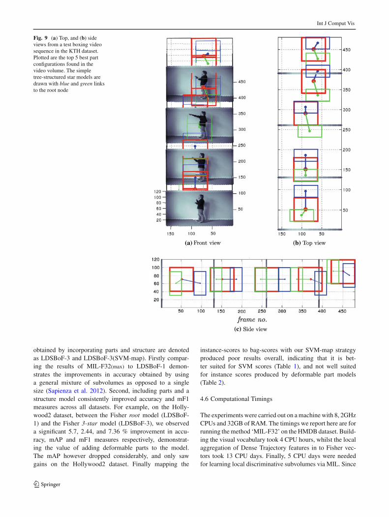
Fig. 9 (a) Top, and (b) sideviews from a test boxing videosequence in the KTH dataset.Plotted are the top 5 best partconfigurations found in thevideo volume. The simpletree-structured star models aredrawn with blue and green linksto the root node

obtained by incorporating parts and structure are denotedas LDSBoF-3 and LDSBoF-3(SVM-map). Firstly compar-ing the results of MIL-F32(max) to LDSBoF-1 demon-strates the improvements in accuracy obtained by usinga general mixture of subvolumes as opposed to a singlesize (Sapienza et al. 2012). Second, including parts and astructure model consistently improved accuracy and mF1measures across all datasets. For example, on the Holly-wood2 dataset, between the Fisher root model (LDSBoF-1) and the Fisher 3-star model (LDSBoF-3), we observeda significant 5.7, 2.44, and 7.36 % improvement in accu-racy, mAP and mF1 measures respectively, demonstrat-ing the value of adding deformable parts to the model.The mAP however dropped considerably, and only sawgains on the Hollywood2 dataset. Finally mapping the

instance-scores to bag-scores with our SVM-map strategyproduced poor results overall, indicating that it is bet-ter suited for SVM scores (Table 1), and not well suitedfor instance scores produced by deformable part models(Table 2).

4.6 Computational Timings

The experiments were carried out on a machine with 8, 2GHzCPUs and 32GB of RAM. The timings we report here are forrunning the method ‘MIL-F32’ on the HMDB dataset. Build-ing the visual vocabulary took 4 CPU hours, whilst the localaggregation of Dense Trajectory features in to Fisher vec-tors took 13 CPU days. Finally, 5 CPU days were neededfor learning local discriminative subvolumes via MIL. Since

123

Int J Comput Vis

the implementation is non optimised in MATLAB, we areconvinced that the computational timings can be cut consid-erably. Note that the low-level feature extraction, the localaggregation, and one-vs-all classification are easily paral-lelised.

4.7 Qualitative Localisation Discussion

In addition to action clip classification, the learnt localinstance models can also be used for action localisation, theresults of which are discussed in the next sections.

4.7.1 Bounding Box Detection with LDSBoF

The LDSBoF approach is able to predict the location of dis-criminative action parts by selecting the top scoring ‘root’and ‘part’ configurations in each video clip. This is clearlyseen in Fig. 9, where the front, top and side views of a boxingvideo sequence from the KTH dataset are plotted in space–time. Notice that the parts correspond to a spatial subdivisionof the root subvolume, and have connections to the root thatare deformable in both space and time.

The space–time plots of Figs. 10a–c show qualitativeresults obtained when detecting actions with LDSBoF mod-els on real-world movie sequences from the Hollywood2dataset. Due to the large variation in video clip length, wepicked the top 5 % detections, which do indeed correspondto discriminative parts of the action; additional examples ofwhich are shown in the attached multimedia material. Thus,our proposed method it is well suited for other action local-isation datasets (Laptev and Pérez 2007; Kläser et al. 2010;Gaidon et al. 2011), which we leave for future work.

4.7.2 Class-Specific Saliency

In contrast to object detection, in which the boundaries of anobject are well defined in space, the ambiguity and inherentvariability of actions means that not all actions are well cap-

Fig. 11 Action classification and localisation on the KTH dataset. (a)This boxing video sequence has been correctly classified as a boxingaction, and has overlaid the boxing action saliency map to indicatethe location of discriminative action parts. (b) This time, the actionclassified is that of a walking action. In this longer video sequence, theactor walks in and out of the camera shot, as shown by the dense redpoints over the locations in which the actor was present in the shot

tured by bounding boxes. As an alternative we propose touse the detection scores as a measure of action location andsaliency, as shown in Fig. 11. Recall that at test-time eachsubvolume is associated with a vector of scores denoting theresponse for each action category in that region. Since in ourframework, we also map the individual instance scores to aglobal video clip classification score (Sect. 3.3), the vectorof scores associated with each subvolume can be reduced tothat of the predicted video action class. It is therefore possi-ble to build an action-specific saliency map by aggregating

Fig. 10 Detected LDSBoF configurations in the challenging Holly-wood2 dataset. The three sequences from the Hollywood2 dataset showthe detections for the videos classified as, (a) GetOutOfCar, (b) Fight-

Person, and (c) StandUp. It is seen that in addition to class labels, eachaction in the video is localised via a 3-part deformable star model

123

Int J Comput Vis

Fig. 12 Action localisation results on the HMDB51 dataset, the mostchallenging action classification dataset to date. In (d), a girl is pouringliquid into a glass, and in (e) a person is pushing a car. Notice thatthe push action does not fire over the person’s moving legs but ratheron the contact zone between the person and the vehicle. Moreover thesaliency map in (b) is focused on the bow and not on the person’s elbowmovement

the predicted detection scores from all instances within thespace–time video. Thus in both Fig. 11a and b, the saliencymap is specific to the predicted global action class, and is dis-played as a sparse set of points for clarity, where the colour,from blue to red, and sparsity of the plotted points indicatethe action class membership strength. Moreover, the saliencymap indicates the action location in both space and time. Inboth videos of Fig. 11, irrelevant scene background, com-mon in most of the KTH classes, was pruned by the MILduring training, and therefore the learnt action models wereable to better detect relevant action instances. Notice that thesaliency map was able to capture both the consistent motionof the boxing action in Fig. 11a, as well as the intermittentwalking action of Fig. 11b.

The qualitative localisation results for the HMDB datasetare shown in Figs. 12 and 13, where the saliency maps drawnover the videos are those corresponding to the predicted

Fig. 13 Misclassifications in the HMDB dataset. The predicted classis shown first, followed by the ground truth class in brackets. Note thatthe localisation scores shown are of the predicted class. (a) A ‘kickball’ action that has frames of Britney Spears singing in the middle.(b) A ‘push’ action wrongly classified as ‘climb’. (c) The fast swingingmovement of the ‘baseball’ action was classified as ‘catch’. (d) A hugwas incorrectly classified as punch, and (e) a ‘punch’ was misclassifiedas ‘clap’. (f) In this case the wave action was misclassified as walk, eventhough President Obama was also walking. The algorithm was unableto cope with the situation in which two actions occur simultaneously

global action class. Note that such a saliency map does notrepresent a general measure of saliency (Vig et al. 2012),rather it is specific to the particular action class being consid-ered. This has the effect of highlighting discriminative partsof the action, for example, in the pushing action of Fig. 12e,the contact between the hands and vehicle is highlighted, lessso the leg’s motion. Likewise in Fig. 12d the pouring actionis highlighted, less so the arm’s motion. The videos of Fig. 13show the results obtained when the clip is incorrectly clas-sified. In this case, higher scores are located at the bordersof the video frame, since the instance scores for the wrongpredicted class are low over the video parts where the actionoccurs. In the HMDB dataset, apart from dealing with a widerange of action classes, our algorithm has to deal with signif-icant nuisance factors in the data, such as frames of ‘BritneySpears’ singing in between a ‘kick_ball’ action (Fig. 13a),and the possibility of multiple actions per video clip such asthe ‘walking’ and ‘waving’ actions in Fig. 13f. Extending theproposed framework in order to deal with multiple actionsper video is left for future work.

5 Conclusion

We proposed a novel general framework for action clip clas-sification and localisation based on the recognition of local

123

Int J Comput Vis

space–time subvolumes. A number of interesting insightsemerged. Our experiments qualitatively demonstrated thatit is possible to localise challenging actions captured ‘in thewild’, with weak annotation, whilst achieving state-of-the-art classification results. Since in our approach the detectionprimitives were space–time subvolumes, there was no needto perform spatial and temporal detection separately (Liuet al. 2009). Rather, each subvolume was associated with alocation in the video, and a decision score for each actionclass.

Even though our method is independent of the choice ofmid-level feature representation, we found that Fisher vec-tors performed the best when compared to kernel-mappedBoF histograms. The experimental results on four majoraction classification datasets further demonstrated that ourlocal subvolume approach outperformed the global baselineon the majority of performance measures. We expect thatby increasing the number of possible subvolumes and thedensity at which they are extracted, we will observe fur-ther improvements in classification and localisation accuracy.Further MIL performance gains may be obtained by multi-ple random initialisations, instead of assigning each instanceto the label of their parent bag, although at higher computa-tional cost. Investigating the importance of each cue in theSVM-map feature vector may also reveal improved mappingstrategies.

Our LDSBoF models coupled with Fisher vectors demon-strated the merits of incorporating action structure into mid-level feature representations, both quantitatively (Table 2)and qualitatively (Fig. 10). By using LDSBoF, we were ableto better model the variability of human actions in space–time, which is reflected in higher performance achieved by a3-part model compared to that of the root filter alone.

In the future, we will focus our attention on describingfurther action detail, such as whether a person is walking fastor slowly, or whether a person jumps high or low, via attributelearning. Furthermore, we plan to move towards denser fea-ture extraction to capture meaningful mid-level representa-tions with smaller subvolumes, extending LDSBoF to a pos-sibly variable and higher number of parts. Moreover we envi-sion initialising part anchor points from the feature distrib-utions to improve over a fixed grid. Our encouraging local-isation results demonstrate the potential for extending thismethod to larger and more challenging localisation datasets.

References

Andrews, S., Tsochantaridis, I., & Hofmann, T. (2003). Support vec-tor machines for multiple-instance learning. In Advances in NeuralInformation Processing Systems.

Blank, M., Gorelick, L., Shechtman, E., Irani, M., & Basri, R. (2005).Actions as space–time shapes. In Proceedings of International Con-ference on Computer Vision (pp. 1395–1402).

Boureau, Y. L., Bach, F., LeCun, Y., & Ponce, J. (2010). Learning mid-level features for recognition. In IEEE International Conference onComputer Vision and Pattern Recognition.

Bronstein, A., Bronstein, M., & Kimmel, R. (2009). Topology-invariantsimilarity of nonrigid shapes. International Journal of ComputerVision, 81(3), 281–301.

Dalal, N., Triggs, B., & Schmid, C. (2006). Human detection using ori-ented histograms of flow and appearance. In Proceedings of Euro-pean Conference Computer Vision.

Dollar, P., Rabaud, V., Cottrell, G., & Belongie, S. (2005). Behaviorrecognition via sparse spatio-temporal features. In Proceedings ofIEEE International Workshop on Visual Surveillance and Perfor-mance Evaluation of Tracking and Surveillance (pp. 65–72).

Duchenne, O., Laptev, I., Sivic, J., Bach, F., & Ponce, J. (2009). Auto-matic annotation of human actions in video. In Proceedings of Inter-national Conference on Computer Vision (pp. 1491–1498).

Felzenszwalb, P., & Huttenlocher, D. (2004). Distance transforms ofsampled functions. Technical report on Cornell Computing and Infor-mation Science.

Felzenszwalb, P., & Huttenlocher, D. (2005). Pictorial structures forobject recognition. International Journal of Computer Vision, 61(1),55–79.

Felzenszwalb, P., Girshick, R., McAllester, D., & Ramanan, D. (2010).Object detection with discriminatively trained part based models.IEEE Transactions on Pattern Analysis and Machine Intelligence,32(9), 1627–1645.

Fischler, M., & Elschlager, R. (1973). The representation and matchingof pictorial structures. IEEE Transactions on Computer, 22(1), 67–92.

Gaidon, A., Harchaoui, Z., & Schmid, C. (2011). Actom sequence mod-els for efficient action detection. In IEEE International Conferenceon Computer Vision and Pattern Recognition.

Gilbert, A., Illingworth, J., & Bowden, R. (2009). Fast realistic multi-action recognition using mined dense spatio-temporal features. InProceedings of International Conference on Computer Vision (pp.925–931).

Jhuang, H., Serre, T., Wolf, L., & Poggio, T. (2007). A biologicallyinspired system for action recognition. In Proceedings of Interna-tional Conference on Computer Vision.

Jiang, Z., Lin, Z., & Davis, L. S. (2012). Recognizing human actions bylearning and matching shape-motion prototype trees. IEEE Transav-tions on Pattern Analysis and Machine Intelligence, 34(3), 533–547.

Ke, Y., Sukthandar, R., & Hebert, M. (2010). Volumetric features forvideo event detection. International Journal of Computer Vision,88(3), 339–362.

Kläser, A., Marszałek, M., & Schmid, C. (2008). A spatio-temporaldescriptor based on 3D-gradients. In Proceedings of British MachineVision Conference.

Kläser, A., Marszałek, M., Schmid, C., & Zisserman, A. (2010). Humanfocused action localization in video. In International Workshop onSign, Gesture, Activity.

Kliper-Gross, O., Gurovich, Y., Hassner, T., & Wolf, L. (2012). Motioninterchange patterns for action recognition in unconstrained videos.InProceedings of European Conference Computer Vision.

Kuehne, H., Jhuang, H., Garrote, E., Poggio, T., & Serre, T. (2011).HMDB: A large video database for human motion recognition. InProceedings of International Conference on Computer Vision.

Laptev, I., & Lindeberg, T. (2003). Space–time interest points. In Pro-ceedings of International Conference on Computer Vision.

Laptev. I., & Pérez, P. (2007). Retrieving actions in movies. In Proceed-ings of International Conference on Computer Vision.

Laptev, I., Marszałek, M., Schmid, C., & Rozenfeld, B. (2008). Learningrealistic human actions from movies. In IEEE International Confer-ence on Computer Vision and Pattern Recognition.

Lazebnik, S., Schmid, C., & Ponce, J. (2006). Beyond bags of features:Spatial pyramid matching for recognizing natural scene categories.

123

Int J Comput Vis

In IEEE International Conference on Computer Vision and PatternRecognition.

Le, Q., Zou, W., Yeung, S., & Ng, A. (2011). Learning hierarchicalinvariant spatio-temporal features for action recognition with inde-pendent subspace analysis. In IEEE International Conference onComputer Vision and Pattern Recognition.

Lin, H. T., Lin, C. J., & Weng, R. C. (2007). A note on platts probabilisticoutputs for support vector machines. Machine Learning, 68(3), 267–276.

Liu, J., Luo, J., & Shah, M. (2009). Recognising realistic actionsfromvideos “in the wild”. In Proceedings of British Machine VisionConference.

Marszałek, M., Laptev, I., & Schmid, C. (2009). Actions in context.In IEEE International Conference on Computer Vision and PatternRecognition.

Muja, M., & Lowe, D. G. (2009). Fast approximate nearest neighborswith automatic algorithm configuration. In VISSAPP (pp. 331–340).

Parizi, S. N., Oberlin, J., & Felzenszwalb, P. (2012). Reconfigurablemodels for scene recognition. In IEEE International Conference onComputer Vision and Pattern Recognition.

Perronnin, F., Sánchez, J., & Mensink, T. (2010). Improving the fisherkernel for large-scale image classification. In Proceedings of Euro-pean Conference Computer Vision.

Perronnin, F., Akata, Z., Harchaoui, Z., & Schmid, C. (2012). Towardsgood practice in large-scale learning for image classification. In IEEEInternational Conference on Computer Vision and Pattern Recogni-tion.

Platt, J. (1999). Probabilistic outputs for support vector machines andcomparisons to regularized likelihood methods. In Advances in largemargin classifiers (Vol. 10(3), pp. 61–74). Cambridge, MA: MITPress

Poppe, R. (2010). A survey on vision-based human action recognition.Image and Vision Computing, 28, 976–990.

Rokhlin, V., Szlam, A., & Tygert, M. (2009). A randomized algorithmfor principal component analysis. SIAM Journal on Matrix Analysisand Applications, 31(3), 1100–1124.

Sapienza, M., Cuzzolin, F., & Torr, P. H. (2012). Learning discriminativespace-time actions from weakly labelled videos. In Proceedings ofBritish Machine Vision Conference.

Schüldt, C., Laptev, I., Caputo, B. (2004). Recognizing human actions:A local SVM approach. In IEEE International Conference on PatternRecognition.

Scovanner, P., Ali, S., & Shah, M. (2007). A 3-dimensional SIFTdescriptor and its application to action recognition. In Proceedingsof ACM Multimedia (pp. 357–360).

Shalev-Shwartz, S., Singer, Y., Srebro, N., & Cotter, A. (2011). Pega-sos: Primal estimated sub-gradient solver for svm. MathematicalProgramming, Series B, 127(1), 3–30.

Vedaldi, A., & Fulkerson, B. (2008). VLFeat: An open and portablelibrary of computer vision algorithms. http://www.vlfeat.org/

Vedaldi, A., & Zisserman, A. (2010). Efficient additive kernels viaexplicit feature maps. In IEEE International Conference on Com-puter Vision and Pattern Recognition.

Vig, E., Dorr, M., & Cox, D. (2012). Space-variant descriptor sam-pling for action recognition based on saliency and eye movements.In Proceedings of European Conference Computer Vision.

Viola, P., Platt, J., & Zhang, C. (2005). Multiple instance boosting forobject detection. In Advances in Neural Information Processing Sys-tems (pp. 1417–1426).

Wang, H., Ullah, M., Kläser, A., Laptev, I., & Schmid, C. (2009). Eval-uation of local spatio-temporal features for action recognition. InProceedings of British Machine Vision Conference.

Wang, H., Kläser, A., Schmid, C., & Liu, C. (2011). Action recognitionby dense trajectories. In IEEE International Conference on ComputerVision and Pattern Recognition.

Weinland, D., Ronfard, R., & Boyer, E. (2011). A survey of vision-basedmethods for action representation, segmentation and recognition.Computer Vision and Image Understanding, 115(2), 224–241.

Willems, G., Tuytelaars, T., & Gool, L. V. (2008). An efficient denseand scale-invariant spatio-temporal interest point detector. In Pro-ceedings of European Conference Computer Vision.

Yeffet, L., & Wolf, L. (2009). Local trinary patterns for human actionrecognition. In Proceedings of International Conference on Com-puter Vision.

123