Free Sample

In this package, you will find: • The author biography • A preview chapter from the book, Chapter 1 ‘Classification in Data Analysis’ • A synopsis of the book’s content • More information on Learning Apache Mahout Classification

About the Author Ashish Gupta has been working in the field of software development for the last 8 years. He has worked in different companies, such as SAP Labs and Caterpillar, as a software developer. While working for a start-up where he was responsible for predicting potential customers for new fashion apparels using social media, he developed an interest in the field of machine learning. Since then, he has worked on using big data technologies and machine learning for different industries, including retail, finance, insurance, and so on. He has a passion for learning new technologies and sharing the knowledge thus gained with others. He has organized many boot camps for the Apache Mahout and Hadoop ecosystem.

First of all, I would like to thank open source communities for their continuous efforts in developing great software for all. I would like to thank Merwyn D'Souza and Reshma Raman, my editors for this project. Special thanks to the reviewers of this book.

Nothing can be accomplished without the support of family, friends, and loved ones. I would like to thank my friends, family, and especially my wife and my son for their continuous support throughout the writing of this book.

Learning Apache Mahout Classification Thanks to the progress made in the hardware industries, our storage capacity has increased, and because of this, there are many organizations who want to store all types of events for analytics purposes. This has given birth to a new era of machine learning. The field of machine learning is very complex and writing these algorithms is not a piece of cake. Apache Mahout provides us with readymade algorithms in the area of machine learning and saves us from the complex task of algorithm implementation.

The intention of this book is to cover classification algorithms available in Apache Mahout. Whether you have already worked on classification algorithms using some other tool or are completely new to the field, this book will help you. So, start reading this book to explore the classification algorithms in one of the most popular open source projects which enjoys strong community support: Apache Mahout.

What This Book Covers Chapter 1, Classification in Data Analysis, provides an introduction to the classification concept in data analysis. This chapter will cover the basics of classification, similarity matrix, and algorithms available in this area.

Chapter 2, Apache Mahout, provides an introduction to Apache Mahout and its installation process. Further, this chapter will talk about why it is a good choice for classification.

Chapter 3, Learning Logistic Regression / SGD Using Mahout, discusses logistic regression and Stochastic Gradient Descent, and how developers can use Mahout to use SGD.

Chapter 4, Learning the Naïve Bayes Classification Using Mahout, discusses the Bayes Theorem, Naïve Bayes classification, and how we can use Mahout to build Naïve Bayes classifier.

Chapter 5, Learning the Hidden Markov Model Using Mahout, covers the HMM and how to use Mahout's HMM algorithms.

Chapter 6, Learning Random Forest Using Mahout, discusses the Random forest algorithm in detail, and how to use Mahout's Random forest implementation.

Chapter 7, Learning Multilayer Perceptron Using Mahout, discusses Mahout as an early level implementation of a neural network. We will discuss Multilayer Perceptron in this chapter. Further, we will use Mahout's implementation of MLP.

Chapter 8, Mahout Changes in the Upcoming Release, discusses Mahout as a work in progress. We will discuss the new major changes in the upcoming release of Mahout.

Chapter 9, Building an E-mail Classification System Using Apache Mahout, provides two use cases of e-mail classification—spam mail classification and e-mail classification based on the project the mail belongs to. We will create the model, and use this model in a program that will simulate the real working environment.

Classifi cation in Data Analysis

In the last decade, we saw a huge growth in social networking and e-commerce sites. I am sure that you must have got information about this book on Facebook, Twitter, or some other site. Chances are also high that you are reading an e-copy of this book after ordering it on your phone or tablet.

This must give you an idea of how much data we are generating over the Internet every single day. Now, in order to obtain all necessary information from the data, we not only create data but also store this data. This data is extremely useful to get some important insights into the business. The analysis of this data can increase the customer base and create profi ts for the organization. Take the example of an e-commerce site. You visit the site to buy some book. You get information about books on related topics or the same topic, publisher, or writer, and this helps you to take better decisions, which also helps the site to know more about its customers. This will eventually lead to an increase in sales.

Finding related items or suggesting a new item to the user is all part of the data science in which we analyze the data and try to get useful patterns.

Data analysis is the process of inspecting historical data and creating models to get useful information that is required to help in decision making. It is helpful in many industries, such as e-commerce, banking, fi nance, healthcare, telecommunications, retail, oceanography, and many more.

Let's take the example of a weather forecasting system. It is a system that can predict the state of the atmosphere at a particular location. In this process, scientists collect historical data of the atmosphere of that location and try to create a model based on it to predict how the atmosphere will evolve over a period of time.

Classifi cation in Data Analysis

[ 8 ]

In machine learning, classifi cation is the automation of the decision-making process that learns from examples of the past and emulates those decisions automatically. Emulating the decisions automatically is a core concept in predictive analytics. In this chapter, we will look at the following points:

• Understanding classifi cation• Working of classifi cation systems• Classifi cation algorithms• Model evaluation methods

Introducing the classifi cationThe word classifi cation always reminds us of our biology class, where we learned about the classifi cation of animals. We learned about different categories of animals, such as mammals, reptiles, birds, amphibians, and so on.

If you remember how these categories are defi ned, you will realize that there were certain properties that scientists found in existing animals, and based on these properties, they categorized a new animal.

Other real-life examples of classifi cation could be, for instance, when you visit the doctor. He/she asks you certain questions, and based on your answers, he/she is able to identify whether you have a certain disease or not.

Classifi cation is the categorization of potential answers, and in machine learning, we want to automate this process. Biological classifi cation is an example of multiclass classifi cation and fi nding the disease is an example of binary classifi cation.

In data analysis, we want to use machine learning concepts. To analyze the data, we want to build a system that can help us to fi nd out which class an individual item belongs to. Usually, these classes are mutually exclusive. A related problem in this area is fi nding out the probability that an individual belongs to a certain class.

Chapter 1

[ 9 ]

Classifi cation is a supervised learning technique. In this technique, machines—based on historical data—learn and gain the capabilities to predict the unknown. In machine learning, another popular technique is unsupervised learning. In supervised learning, we already know the output categories, but in unsupervised learning, we know nothing about the output. Let's understand this with a quick example: suppose we have a fruit basket, and we want to classify fruits. When we say classify, it means that in the training data, we already have output variables, such as size and color, and we know whether the color is red and the size is from 2.3" to 3.7". We will classify that fruit as an apple. Opposite to this, in unsupervised learning, we want to separate different fruits, and we do not have any output information in the training dataset, so the learning algorithm will separate different fruits based on different features present in the dataset, but it will not be able to label them. In other words, it will not be able to tell which one is an apple and which one is a banana, although it will be able to separate them.

Application of the classifi cation systemClassifi cation is used for prediction. In the case of e-mail categorization, it is used to classify e-mail as spam or not spam. Nowadays, Gmail is classifying e-mails as primary, social, and promotional as well. Classifi cation is useful in predicting credit card frauds, to categorize customers for eligibility of loans, and so on. It is also used to predict customer churn in the insurance and telecom industries. It is useful in the healthcare industry as well. Based on historical data, it is useful in classifying particular symptoms of a disease to predict the disease in advance. Classifi cation can be used to classify tropical cyclones. So, it is useful across all industries.

Working of the classifi cation systemLet's understand the classifi cation process in more detail. In the process of classifi cation, with the dataset given to us, we try to fi nd out informative variables using which we can reduce the uncertainty and categorize something. These informative variables are called explanatory variables or features.

Classifi cation in Data Analysis

[ 10 ]

The fi nal categories that we are interested are called target variables or labels. Explanatory variables can be any of the following forms:

• Continuous (numeric types)• Categorical• Word-like• Text-like

If numeric types are not useful for any mathematical functions, those will be counted as categorical (zip codes, street numbers, and so on).

So, for example, we have a dataset of customer's' loan applications, and we want to build a classifi er to fi nd out whether a new customer is eligible for a loan or not. In this dataset, we can have the following fi elds:

• Customer Age• Customer Income (PA)• Customer Account Balance• Loan Granted

From these fi elds, Customer Age, Customer Income (PA) and Customer Account Balance will work as explanatory variables and Loan Granted will be the target variable, as shown in the following screenshot:

Chapter 1

[ 11 ]

To understand the creation of the classifi er, we need to understand a few terms, as shown in the following diagram:

• Training dataset: From the given dataset, a portion of the data is used to create the training dataset (it could be 70 percent of the given data). This dataset is used to build the classifi er. All the feature sets are used in this dataset.

• Test dataset: The dataset that is left after the training dataset is used to test the created model. With this data, only the feature set is used and the model is used to predict the target variables or labels.

• Model: This is used to understand the algorithm used to generate the target variables.

While building a classifi er, we follow these steps:

• Collecting historical data• Cleaning data (a lot of activities are involved here, such as space removal,

and so on)

Classifi cation in Data Analysis

[ 12 ]

• Defi ning target variables• Defi ning explanatory variables• Selecting an algorithm• Training the model (using the training dataset)• Running test data• Evaluating the model• Adjusting explanatory variables• Rerunning the test

While preparing the model, one should take care of outlier detection. Outlier detection is a method to fi nd out items that do not conform to an expected pattern in a dataset. Outliers in an input dataset can mislead the training process of an algorithm. This can affect the model accuracy. There are algorithms to fi nd out these outliers in the datasets. Distance-based techniques and fuzzy-logic-based methods are mostly used to fi nd out outliers in the dataset. Let's talk about one example to understand the outliers.

We have a set of numbers, and we want to fi nd out the mean of these numbers:

10, 75, 10, 15, 20, 85, 25, 30, 25

Just plot these numbers and the result will be as shown in the following screenshot:

Clearly, the numbers 75 and 85 are outliers (far away in the plot from the other numbers).

Mean = sum of values/number of values = 32.78

Mean without the outliers: = 19.29

So, now you can understand how outliers can affect the results.

While creating the model, we can encounter two majorly occurring problems—Overfi tting and Underfi tting.

Chapter 1

[ 13 ]

Overfi tting occurs when the algorithm captures the noise of the data, and the algorithm fi ts the data too well. Generally, it occurs if we use all the given data to build the model using pure memorization. Instead of fi nding out the generalizing pattern, the model just memorizes the pattern. Usually, in the case of overfi tting, the model gets more complex, and it is allowed to pick up spurious correlations. These correlations are specifi c to training datasets and do not represent characteristics of the whole dataset in general.

The following diagram is an example of overfi tting. An outlier is present, and the algorithm considers that and creates a model that perfectly classifi es the training set, but because of this, the test data is wrongly classifi ed (both the rectangles are classifi ed as stars in the test data):

There is no single method to avoid overfi tting; however, we have some approaches, such as a reduction in the number of features and the regularization of a few of the features. Another way is to train the model with some dataset and test with the remaining dataset. A common method called cross-validation is used to generate multiple performance measures. In this way, a single dataset is split and used for the creation of performance measures.

Underfi tting occurs when the algorithm cannot capture the patterns in the data, and the data does not fi t well. Underfi tting is also known as high bias. It means your algorithm has such a strong bias towards its hypothesis that it does not fi t the data well. For an underfi tting error, more data will not help. It can increase the training error. More explanatory variables can help to deal with the underfi tting problem. More explanatory fi elds will expand the hypothesis space and will be useful to overcome this problem.

Both overfi tting and underfi tting provide poor results with new datasets.

Classifi cation in Data Analysis

[ 14 ]

Classifi cation algorithmsWe will now discuss the following algorithms that are supported by Apache Mahout in this book:

• Logistic regression / Stochastic Gradient Descent (SGD): We usually read regression along with classifi cation, but actually, there is a difference between the two. Classifi cation involves a categorical target variable, while regression involves a numeric target variable. Classifi cation predicts whether something will happen, and regression predicts how much of something will happen. We will cover this algorithm in Chapter 3, Learning Logistic Regression / SGD Using Mahout. Mahout supports logistic regression trained via Stochastic Gradient Descent.

• Naïve Bayes classifi cation: This is a very popular algorithm for text classifi cation. Naïve Bayes uses the concept of probability to classify new items. It is based on the Bayes theorem. We will discuss this algorithm in Chapter 4, Learning the Naïve Bayes Classifi cation Using Mahout. In this chapter, we will see how Mahout is useful in classifying text, which is required in the data analysis fi eld. We will discuss vectorization, bag of words, n-grams, and other terms used in text classifi cation.

• Hidden Markov Model (HMM): This is used in various fi elds, such as speech recognition, parts-of-speech tagging, gene prediction, time-series analysis, and so on. In HMM, we observe a sequence of emissions but do not have a sequence of states which a model uses to generate the emission. In Chapter 5, Learning the Hidden Markov Model Using Mahout, we will take one more algorithm supported by Mahout Hidden Markov Model. We will discuss HMM in detail and see how Mahout supports this algorithm.

• Random Forest: This is the most widely used algorithm in classifi cation. Random Forest consists of a collection of simple tree predictors, each capable of producing a response when presented with a set of explanatory variables. In Chapter 6, Learning Random Forest Using Mahout, we will discuss this algorithm in detail and also talk about how to use Mahout to implement this algorithm.

• Multi-layer Perceptron (MLP): In Chapter 7, Learning Multilayer Perceptron Using Mahout, we will discuss this newly implemented algorithm in Mahout. An MLP consists of multiple layers of nodes in a directed graph, with each layer fully connected to the next one. It is a base for the implementation of neural networks. We will discuss neural networks a little but only after a detailed discussion on MLP in Mahout.

Chapter 1

[ 15 ]

We will discuss all the classifi cation algorithms supported by Apache Mahout in this book, and we will also check the model evaluation techniques provided by Apache Mahout.

Model evaluation techniquesWe cannot have a single evaluation metric that can fi t all the classifi er models, but we can fi nd out some common issues in evaluation, and we have techniques to deal with them. We will discuss the following techniques that are used in Mahout:

• Confusion matrix• ROC graph• AUC• Entropy matrix

The confusion matrixThe confusion matrix provides us with the number of correct and incorrect predictions made by the model compared with the actual outcomes (target values) in the data. A confusion matrix is a N*N matrix, where N is the number of labels (classes). Each column is an instance in the predicted class, and each row is an instance in the actual class. Using this matrix, we can fi nd out how one class is confused with another. Let's assume that we have a classifi er that classifi es three fruits: strawberries, cherries, and grapes. Assuming that we have a sample of 24 fruits: 7 strawberries, 8 cherries, and 9 grapes, the resulting confusion matrix will be as shown in the following table:

Predicted classes by model

Actual class

Strawberries Cherries GrapesStrawberries 4 3 0Cherries 2 5 1Grapes 0 1 8

So, in this model, from the 8 strawberries, 3 were classifi ed as cherries. From the 8 cherries, 2 were classifi ed as strawberries, and 1 is classifi ed as a grape. From the 9 grapes, 1 is classifi ed as a cherry. From this matrix, we will create the table of confusion. The table of confusion has two rows and two columns that report about true positive, true negative, false positive, and false negative.

Classifi cation in Data Analysis

[ 16 ]

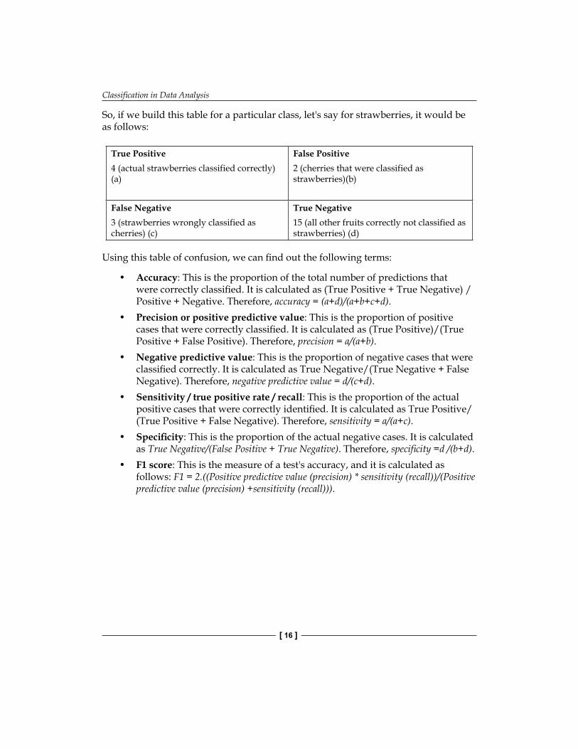
So, if we build this table for a particular class, let's say for strawberries, it would be as follows:

True Positive4 (actual strawberries classified correctly) (a)

False Positive2 (cherries that were classified as strawberries)(b)

False Negative3 (strawberries wrongly classified as cherries) (c)

True Negative15 (all other fruits correctly not classified as strawberries) (d)

Using this table of confusion, we can fi nd out the following terms:

• Accuracy: This is the proportion of the total number of predictions that were correctly classifi ed. It is calculated as (True Positive + True Negative) / Positive + Negative. Therefore, accuracy = (a+d)/(a+b+c+d).

• Precision or positive predictive value: This is the proportion of positive cases that were correctly classifi ed. It is calculated as (True Positive)/(True Positive + False Positive). Therefore, precision = a/(a+b).

• Negative predictive value: This is the proportion of negative cases that were classifi ed correctly. It is calculated as True Negative/(True Negative + False Negative). Therefore, negative predictive value = d/(c+d).

• Sensitivity / true positive rate / recall: This is the proportion of the actual positive cases that were correctly identifi ed. It is calculated as True Positive/(True Positive + False Negative). Therefore, sensitivity = a/(a+c).

• Specifi city: This is the proportion of the actual negative cases. It is calculated as True Negative/(False Positive + True Negative). Therefore, specifi city =d /(b+d).

• F1 score: This is the measure of a test's accuracy, and it is calculated as follows: F1 = 2.((Positive predictive value (precision) * sensitivity (recall))/(Positive predictive value (precision) +sensitivity (recall))).

Chapter 1

[ 17 ]

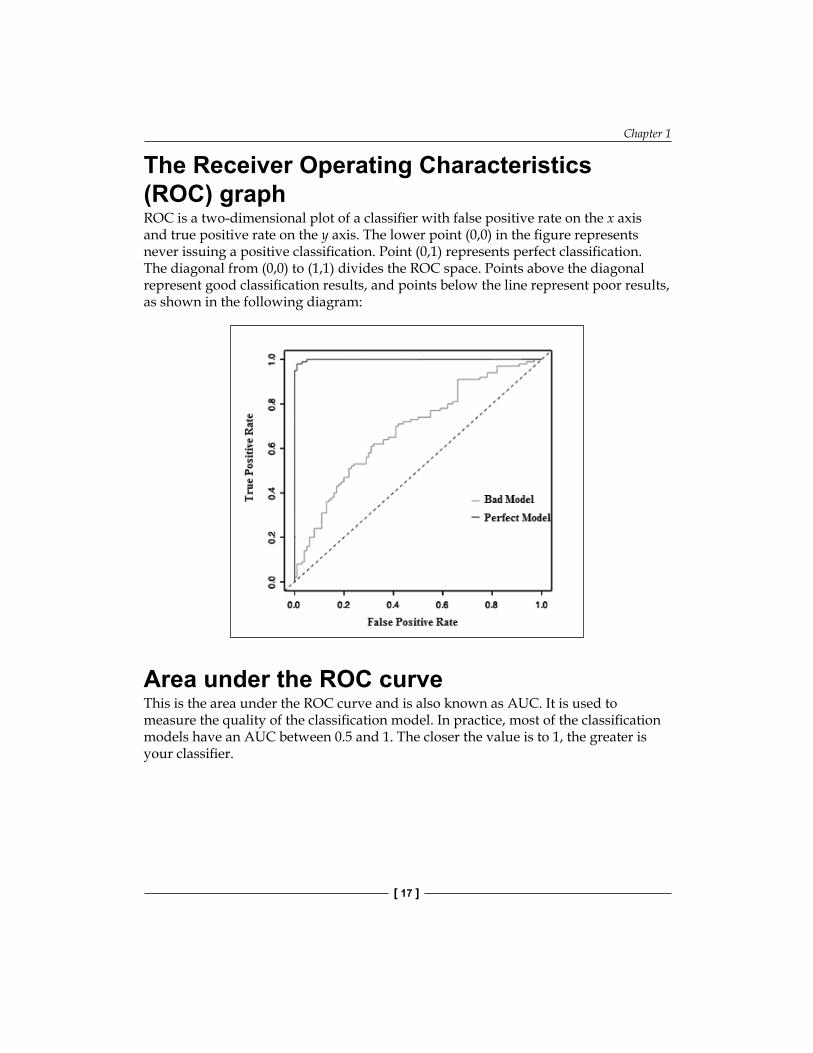
The Receiver Operating Characteristics (ROC) graphROC is a two-dimensional plot of a classifi er with false positive rate on the x axis and true positive rate on the y axis. The lower point (0,0) in the fi gure represents never issuing a positive classifi cation. Point (0,1) represents perfect classifi cation. The diagonal from (0,0) to (1,1) divides the ROC space. Points above the diagonal represent good classifi cation results, and points below the line represent poor results, as shown in the following diagram:

Area under the ROC curveThis is the area under the ROC curve and is also known as AUC. It is used to measure the quality of the classifi cation model. In practice, most of the classifi cation models have an AUC between 0.5 and 1. The closer the value is to 1, the greater is your classifi er.

Classifi cation in Data Analysis

[ 18 ]

The entropy matrixBefore going into the details of the entropy matrix, fi rst we need to understand entropy. The concept of entropy in information theory was developed by Shannon.

Entropy is a measure of disorder that can be applied to a set. It is defi ned as:

Entropy = -p1log(p1) – p2log(p2)- …….

Each p is the probability of a particular property within the set. Let's revisit our customer loan application dataset. For example, assuming we have a set of 10 customers from which 6 are eligible for a loan and 4 are not. Here, we have two properties (classes): eligible or not eligible.

P(eligible) = 6/10 = 0.6

P(not eligible) = 4/10 = 0.4

So, entropy of the dataset will be:

Entropy = -[0.6*log2(0.6)+0.4*log2(0.4)]

= -[0.6*-0.74 +0.4*-1.32]

= 0.972

Entropy is useful in acquiring knowledge of information gain. Information gain measures the change in entropy due to any new information being added in model creation. So, if entropy decreases from new information, it indicates that the model is performing well now. Information gain is calculated as:

IG (classes , subclasses) = entropy(class) –(p(subclass1)*entropy(subclass1)+ p(subclass2)*entropy(subclass2) + …)

Entropy matrix is basically the same as the confusion matrix defi ned earlier; the only difference is that the elements in the matrix are the averages of the log of the probability score for each true or estimated category combination. A good model will have small negative numbers along the diagonal and will have large negative numbers in the off-diagonal position.

Chapter 1

[ 19 ]

SummaryWe have discussed classifi cation and its applications and also what algorithm and classifi er evaluation techniques are supported by Mahout. We discussed techniques like confusion matrix, ROC graph, AUC, and entropy matrix.

Now, we will move to the next chapter and set up Apache Mahout and the developer environment. We will also discuss the architecture of Apache Mahout and fi nd out why Mahout is a good choice for classifi cation.

Where to buy this book You can buy Learning Apache Mahout Classification from the Packt Publishing website. Alternatively, you can buy the book from Amazon, BN.com, Computer Manuals and most internet book retailers.

Click here for ordering and shipping details.

www.PacktPub.com

Stay Connected:

Get more information Learning Apache Mahout Classification