Journal of Machine Learning Research 17 (2016) 1-25 Submitted 12/14; Revised 8/15; Published 4/16

Learning Algorithms for Second-Price Auctions with Reserve

Mehryar Mohri and Andres Munoz MedinaCourant Institute of Mathematical Sciences251 Mercer StreetNew York, NY, 10012

Editor: Kevin Murphy

AbstractSecond-price auctions with reserve play a critical role in the revenue of modern search engine and popularonline sites since the revenue of these companies often directly depends on the outcome of such auctions. Thechoice of the reserve price is the main mechanism through which the auction revenue can be influenced inthese electronic markets. We cast the problem of selecting the reserve price to optimize revenue as a learningproblem and present a full theoretical analysis dealing with the complex properties of the corresponding lossfunction. We further give novel algorithms for solving this problem and report the results of several experi-ments in both synthetic and real-world data demonstrating their effectiveness.

Keywords: Learning Theory, Auctions, Revenue Optimization

1. IntroductionOver the past few years, advertisement has gradually moved away from the traditional printed promotionto the more tailored and directed online publicity. The advantages of online advertisement are clear: sincemost modern search engine and popular online site companies such as Microsoft, Facebook, Google, eBay, orAmazon may collect information about the users’ behavior, advertisers can better target the population sectorfor which their brand is intended.

More recently, a new method for selling advertisements has gained momentum. Unlike the standardcontracts between publishers and advertisers where some amount of impressions are required to be fulfilledby the publisher, an Ad Exchange works in a way similar to a financial exchange where advertisers bid andcompete between each other for an ad slot. The winner then pays the publisher and his ad is displayed.

The design of such auctions and their properties are crucial since they generate a large fraction of therevenue of popular online sites. These questions have motivated extensive research on the topic of auctioningin the last decade or so, particularly in the theoretical computer science and economic theory communities.Much of this work has focused on the analysis of mechanism design, either to prove some useful property ofan existing auctioning mechanism, to analyze its computational efficiency, or to search for an optimal revenuemaximization truthful mechanism (see Muthukrishnan (2009) for a good discussion of key research problemsrelated to Ad Exchange and references to a fast growing literature therein).

One particularly important problem is that of determining an auction mechanism that achieves optimalrevenue (Muthukrishnan, 2009). In the ideal scenario where the valuation of the bidders is drawn i.i.d. froma given distribution, this is known to be achievable (see for example (Myerson, 1981)). But, even goodapproximations of such distributions are not known in practice. Game theoretical approaches to the design ofauctions have given a series of interesting results including (Riley and Samuelson, 1981; Milgrom and Weber,1982; Myerson, 1981; Nisan et al., 2007), all of them based on some assumptions about the distribution of thebidders, e.g., the monotone hazard rate assumption.

The results of these publications have set the basis for most Ad Exchanges in practice: the mechanismwidely adopted for selling ad slots is that of a Vickrey auction (Vickrey, 1961) or second-price auction withreserve price (Easley and Kleinberg, 2010). In such auctions, the winning bidder (if any) pays the maximumof the second-place bid and the reserve price. The reserve price can be set by the publisher or automaticallyby the exchange. The popularity of these auctions relies on the fact that they are incentive-compatible, i.e.,

c©2016 Mehryar Mohri, Andres Munoz Medina.

MOHRI AND MUNOZ MEDINA

bidders bid exactly what they are willing to pay. It is clear that the revenue of the publisher depends greatlyon how the reserve price is set: if set too low, the winner of the auction might end up paying only a smallamount, even if his bid was high; on the other hand, if it is set too high, then bidders may not bid higher thanthe reserve price and the ad slot will not be sold.

We propose a learning approach to the problem of determining the reserve price to optimize revenue insuch auctions. The general idea is to leverage the information gained from past auctions to predict a beneficialreserve price. Since every transaction on an Exchange is logged, it is natural to seek to exploit that data. Thiscould be used to estimate the probability distribution of the bidders, which can then be used indirectly to comeup with the optimal reserve price (Myerson, 1981; Ostrovsky and Schwarz, 2011). Instead, we will seek adiscriminative method making use of the loss function related to the problem and taking advantage of existinguser features.

Learning methods have been used in the past for the related problems of designing incentive-compatibleauction mechanisms (Balcan et al., 2008; Blum et al., 2004), for algorithmic bidding (Langford et al., 2010;Amin et al., 2012), and even for predicting bid landscapes (Cui et al., 2011). Another closely related problemfor which machine learning solutions have been proposed is that of revenue optimization for sponsored searchads and click-through rate predictions (Zhu et al., 2009; He et al., 2013; Devanur and Kakade, 2009). But, toour knowledge, no prior work has used historical data in combination with user features for the sole purposeof revenue optimization in this context. In fact, the only publications we are aware of that are directly relatedto our objective are (Ostrovsky and Schwarz, 2011) and (Cesa-Bianchi et al., 2013), which considers a moregeneral case than (Ostrovsky and Schwarz, 2011).

The scenario studied by Cesa-Bianchi et al. (2013) is that of censored information, which motivates theiruse of a regret minimization algorithm to optimize the revenue of the seller. Our analysis assumes insteadaccess to full information. We argue that this is a more realistic scenario since most companies do have accessto the full historical data. The learning scenario we consider is also more general since it includes the useof features, as is standard in supervised learning. Since user information is communicated to advertisers andbids are made based on that information, it is only natural to include user features in the formulation of thelearning problem. A special case of our analysis coincides with the no-feature scenario considered by Cesa-Bianchi et al. (2013), assuming full information. But, our results further extend those of this paper even in thatscenario. In particular, we present an O(m logm) algorithm for solving a key optimization problem used asa subroutine by these authors, for which they do not seem to give an algorithm. We also do not assume thatbuyers’ bids are sampled i.i.d. from a common distribution. Instead, we only assume that the full outcome ofeach auction is independent and identically distributed. This subtle distinction makes our scenario closer toreality as it is unlikely for all bidders to follow the same underlying value distribution. Moreover, even thoughour scenario does not take into account a possible strategic behavior of bidders between rounds, it allows forbidders to be correlated, which is common in practice.

This paper is organized as follows: in Section 2, we describe the setup and give a formal descriptionof the learning problem. We discuss the relations between the scenario we consider and previous work onlearning in auctions in Section 3. In particular, we show that, unlike previous work, our problem can be castas that of minimizing the expected value of a loss function, which is a standard learning problem. Unlike mostwork in this field, however, the loss function naturally associated to this problem does not admit favorableproperties such as convexity or Lipschitz continuity. In fact the loss function is discontinuous. Therefore, thetheoretical and algorithmic analysis of this problem raises several non-trivial technical issues. Nevertheless,we use a decomposition of the loss to derive generalization bounds for this problem (see Section 4). Thesebounds suggest the use of structural risk minimization to determine a learning solution benefiting from strongguarantees. This, however, poses a new challenge: solving a highly non-convex optimization problem. Similaralgorithmic problems have been of course previously encountered in the learning literature, most notably whenseeking to minimize a regularized empirical 0-1 loss in binary classification. A standard method in machinelearning for dealing with such issues consists of resorting to a convex surrogate loss (such as the hinge losscommonly used in linear classification). However, we show in Section 4.2 that no convex loss function iscalibrated for the natural loss function for this problem. That is, minimizing a convex surrogate could bedetrimental to learning. This fact is further empirically verified in Section 6.

The impossibility results of Section 4.2 prompt us to search for surrogate loss functions with weakerregularity properties such as Lipschitz continuity. We describe a loss function with precisely that propertywhich we further show to be consistent with the original loss. We also provide finite sample learning guar-antees for that loss function, which suggest minimizing its empirical value while controlling the complexity

2

LEARNING IN SECOND-PRICE AUCTIONS WITH RESERVE

of the hypothesis set. This leads to an optimization problem which, albeit non-convex, admits a favorabledecomposition as a difference of two convex functions (DC-programming). Thus, we suggest using the DC-programming algorithm (DCA) introduced by Tao and An (1998) to solve our optimization problem. Thisalgorithm admits favorable convergence guarantees to a local minimum. To further improve upon DCA, wepropose a combinatorial algorithm to cycle through different local minima with the guarantee of reducing theobjective function at every iteration. Finally, in Section 6, we show that our algorithm outperforms severaldifferent baselines in various synthetic and real-world revenue optimization tasks.

2. SetupWe start with the description of the problem and our formulation of the learning setup. We study second-priceauctions with reserve, the type of auctions adopted in many Ad Exchanges. In such auctions, the bidderssubmit their bids simultaneously and the winner, if any, pays the maximum of the value of the second-placebid and a reserve price r set by the seller. This type of auctions benefits from the same truthfulness property assecond-price auctions (or Vickrey auctions) Vickrey (1961): truthful bidding can be shown to be a dominantstrategy in such auctions. The choice of the reserve price r is the only mechanism through which the seller caninfluence the auction revenue. Its choice is thus critical: if set too low, the amount paid by the winner could betoo small; if set too high, the ad slot could be lost. How can we select the reserve price to optimize revenue?

We consider the problem of learning to set the reserve prices to optimize revenue in second-price auctionswith reserve. The outcome of an auction can be encoded by the highest and second-highest bids which wedenote by a vector b = (b(1), b(2)) ∈ B ⊂ R2

+. We will assume that there exists an upper bound M ∈(0,+∞) for the bids: supb∈B b

(1) = M . For a given reserve price r and bid pair b, by definition, the revenueof an auction is given by

Revenue(r,b) = b(2)1r<b(2) + r1b(2)≤r≤b(1) .

We consider the general scenario where a feature vector x ∈ X ⊂ RN is associated with each auction. Inthe auction theory literature, this feature vector is commonly referred to as public information. In the contextof online advertisement, this could be for example information about the user’s location, gender or age. Thelearning problem can thus be formulated as that of selecting out of a hypothesis set H of functions mappingX to R a hypothesis h with high expected revenue

E(x,b)∼D

[Revenue(h(x),b)], (1)

whereD is an unknown distribution according to which pairs (x,b) are drawn. Instead of the revenue, we willconsider a loss function L defined for all (r,b) by L(r,b) = −Revenue(r,b), and will equivalently seek ahypothesis h with small expected loss L(h) := E(x,b)∼D[L(h(x),b)]. As in standard supervised learningscenarios, we assume access to a training sample S = ((x1,b1), . . . , (xm,bm)) of size m ≥ 1 drawn i.i.d.according to D. We will denote by LS(h) the empirical loss LS(h) = 1

m

∑mi=1 L(h(xi,bi)). Notice that

we only assume that the auction outcomes are i.i.d. and not that bidders are independent of each other withthe same underlying bid distribution, as in some previous work (Cesa-Bianchi et al., 2013; Ostrovsky andSchwarz, 2011). In the next sections, we will present a detailed study of this learning problem, starting with areview of the related literature.

3. Previous workHere, we briefly discuss some previous work related to the study of auctions from a learning standpoint. One ofthe earliest contributions in this literature is that of Blum et al. (2004) where the authors studied a posted-priceauction mechanism where a seller offers some good at a certain price and where the buyer decides to eitheraccept that price or reject it. It is not hard to see that this type of auctions is equivalent to second-price auctionswith reserve with a single buyer. The authors consider a scenario of repeated interactions with different buyerswhere the goal is to design an incentive-compatible method of setting prices that is competitive with the bestfixed-priced strategy in hindsight. A fixed-price strategy is one that simply offers the same price to all buyers.Using a variant of the EXP3 algorithm of Auer et al. (2002), the authors designed a pricing algorithm achievinga (1+ ε)-approximation to the best fixed-price strategy. This same scenario was also studied by Kleinberg andLeighton (2003) who gave an online algorithm whose regret after T rounds is in O(T 2/3).

3

MOHRI AND MUNOZ MEDINA

A step further in the design of optimal pricing strategies was proposed by Balcan et al. (2008). One ofthe problems considered by the authors was that of setting prices for n buyers in a posted-price auction as afunction of their public information. Unlike the on-line scenario of Blum et al. (2004), Balcan et al. (2008)considered a batch scenario where all buyers are known in advance. However, the comparison class consideredwas no longer that of simple fixed-price strategies but functions mapping public information to prices. Thismakes the problem more challenging and closer to the scenario we consider. The authors showed that findinga (1 + ε)-optimal truthful mechanism is equivalent to finding an algorithm to optimize the empirical riskassociated to the loss function we consider (in the case b(2) ≡ 0). There are multiple connections between thiswork and our results. In particular, the authors pointed out that the discontinuity and asymmetry of the lossfunction presented several challenges to their analysis. We will see that, in fact, the same problems appear inthe derivation of our learning guarantees. But, we will present an algorithm for minimizing the empirical riskwhich was a crucial element missing in their results.

A different line of work by Cui et al. (2011) focused on predicting the highest bid of a second-price auction.To estimate the distribution of the highest bid, the authors partitioned the space of advertisers based on theircampaign objectives and estimated the distribution for each partition. Within each partition, the distribution ofthe highest bid was modeled as a mixture of log-normal distributions where the means and standard deviationsof the mixtures were estimated as a function of the data features. While it may seem natural to seek to predictthe highest bid, we show that this is not necessary and that accurate predictions of the highest bid do notnecessarily translate into algorithms achieving large revenue (see Section 6).

As already mentioned, the closest previous work to ours is that of Cesa-Bianchi et al. (2013), who studiedthe problem of directly optimizing the revenue under a partial information setting where the learner can onlyobserve the value of the second-highest bid, if it is higher than the reserve price. In particular, the highest bidremains unknown to the learner. This is a natural scenario for auctions such as those of eBay where only theprice at which an object is sold is reported. To do so, the authors expressed the expected revenue in terms ofthe quantity q(t) = P[b(2) > t]. This can be done as follows:

Eb

[Revenue(r,b)] = Eb(2)

[b(2)1r<b(2) ] + r P[b(2) ≤ r ≤ b(1)] (2)

=

∫ +∞

0

P[b(2)1r<b(2) > t] dt+ r P[b(2) ≤ r ≤ b(1)]

=

∫ r

0

P[r < b(2)] dt+

∫ ∞r

P[b(2) > t]dt+ r P[b(2) ≤ r ≤ b(1)]

=

∫ ∞r

P[b(2) > t] dt+ r(P[b(2) > r] + 1− P[b(2) > r]− P[b(1) < r])

=

∫ ∞r

P[b(2) > t] dt+ r P[b(1) ≥ r].

The main observation of Cesa-Bianchi et al. (2013) was that the quantity q(t) can be estimated from theobserved outcomes of previous auctions. Furthermore, if the buyers’ bids are i.i.d., then, one can expressP[b(1) ≥ r] as a function of the estimated value of q(r). This implies that the right-hand side of (2) can beaccurately estimated and therefore an optimal reserve price can be selected. Their algorithm makes calls toa procedure that maximizes the empirical revenue. The authors, however, did not describe an algorithm forthat maximization. A by-product of our work is an efficient algorithm for that procedure. The guarantees ofCesa-Bianchi et al. (2013) are similar to those presented in the next section in the special case of learningwithout features. However, our derivation is different since we consider a batch scenario while Cesa-Bianchiet al. (2013) treated an online setup for which they presented regret guarantees.

4. Learning GuaranteesThe problem we consider is an instance of the well known family of supervised learning problems. However,the loss function L does not admit any of the properties such as convexity or Lipschitz continuity often as-sumed in the analysis of the generalization error, as shown by Figure 1(a). Furthermore, L is discontinuousand, unlike the 0-1 loss function whose discontinuity point is independent of the label, its discontinuity de-pends on the outcome b of the auction. Thus, the problem of learning with the loss function L requires a newanalysis.

4

LEARNING IN SECOND-PRICE AUCTIONS WITH RESERVE

0 1 2 3 4 5 6 7-5

-4

-3

-2

-1

0

b(1)

b(2)

−b(2)

0 1 2 3 4 5 6 7-5

-4

-3

-2

-1

0

b(1)

b(2)

−b(2)

0 1 2 3 4 5 6 7-1

0

1

2

3

4

b(1)

(a) (b)

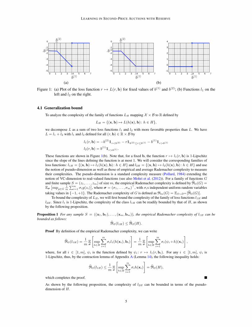
Figure 1: (a) Plot of the loss function r 7→ L(r,b) for fixed values of b(1) and b(2); (b) Functions l1 on theleft and l2 on the right.

4.1 Generalization bound

To analyze the complexity of the family of functions LH mapping X × B to R defined by

LH = {(x,b) 7→ L(h(x),b) : h ∈ H},

we decompose L as a sum of two loss functions l1 and l2 with more favorable properties than L. We haveL = l1 + l2 with l1 and l2 defined for all (r,b) ∈ R× B by

l1(r,b) = −b(2)1r<b(2) − r1b(2)≤r≤b(1) − b

(1)1r>b(1)

l2(r,b) = b(1)1r>b(1) .

These functions are shown in Figure 1(b). Note that, for a fixed b, the function r 7→ l1(r,b) is 1-Lipschitzsince the slope of the lines defining the function is at most 1. We will consider the corresponding families ofloss functions: l1H = {(x,b) 7→ l1(h(x),b) : h ∈ H} and l2H = {(x,b) 7→ l2(h(x),b) : h ∈ H} and usethe notion of pseudo-dimension as well as those of empirical and average Rademacher complexity to measuretheir complexities. The pseudo-dimension is a standard complexity measure (Pollard, 1984) extending thenotion of VC-dimension to real-valued functions (see also Mohri et al. (2012)). For a family of functions Gand finite sample S = (z1, . . . , zm) of size m, the empirical Rademacher complexity is defined by RS(G) =Eσ

[supg∈G

1m

∑mi=1 σig(zi)

], where σ = (σ1, . . . , σm)>, with σis independent uniform random variables

taking values in {−1,+1}. The Rademacher complexity of G is defined as Rm(G) = ES∼Dm [RS(G)].To bound the complexity of LH , we will first bound the complexity of the family of loss functions l1H and

l2H . Since l1 is 1-Lipschitz, the complexity of the class l1H can be readily bounded by that of H , as shownby the following proposition.

Proposition 1 For any sample S = ((x1,b1), . . . , (xm,bm)), the empirical Rademacher complexity of l1H can bebounded as follows:

RS(l1H) ≤ RS(H).

Proof By definition of the empirical Rademacher complexity, we can write

RS(l1H) =1

mEσ

[suph∈H

m∑i=1

σil1(h(xi),bi)

]=

1

mEσ

[suph∈H

m∑i=1

σi(ψi ◦ h)(xi)

],

where, for all i ∈ [1,m], ψi is the function defined by ψi : r 7→ l1(r,bi). For any i ∈ [1,m], ψi is1-Lipschitz, thus, by the contraction lemma of Appendix A (Lemma 14), the following inequality holds:

RS(l1H) ≤ 1

mEσ

[suph∈H

m∑i=1

σih(xi)

]= RS(H),

which completes the proof.

As shown by the following proposition, the complexity of l2H can be bounded in terms of the pseudo-dimension of H .

5

MOHRI AND MUNOZ MEDINA

Proposition 2 Let d = Pdim(H) denote the pseudo-dimension ofH , then, for any sample S=((x1,b1), . . . , (xm,bm)),the empirical Rademacher complexity of l2H can be bounded as follows:

RS(l2H) ≤M√

2d log emd

m.

Proof By definition of the empirical Rademacher complexity, we can write

RS(l2H) =1

mEσ

[suph∈H

m∑i=1

σib(1)i 1

h(xi)>b(1)i

]=

1

mEσ

[suph∈H

m∑i=1

σiΨi(1h(xi)>b(1)i

)

],

where, for all i ∈ [1,m], Ψi is the M -Lipschitz function x 7→ b(1)i x. Thus, by Lemma 14 combined with

Massart’s lemma (see for example Mohri et al. (2012)), we can write

RS(l2H) ≤ M

mEσ

[suph∈H

m∑i=1

σi1h(xi)>b(1)i

]≤M

√2d′ log em

d′

m,

where d′ = VCdim({(x,b) 7→ 1h(x)−b(1)>0 : (x,b) ∈ X × B}). Since the second bid component b(2)

plays no role in this definition, d′ coincides with VCdim({(x, b(1)) 7→ 1h(x)−b(1)>0 : (x, b(1)) ∈ X × B1}),where B1 is the projection of B ⊆ R2 onto its first component, and is upper-bounded by VCdim({(x, t) 7→1h(x)−t>0 : (x, t) ∈ X × R}), that is, the pseudo-dimension of H .

Propositions 1 and 2 can be used to derive the following generalization bound for the learning problem weconsider.

Theorem 3 For any δ > 0, with probability at least 1 − δ over the draw of an i.i.d. sample S of size m, the followinginequality holds for all h ∈ H:

L(h) ≤ LS(h) + 2Rm(H) + 2M

√2d log em

d

m+M

√log 1

δ

2m.

Proof By a standard property of the Rademacher complexity, sinceL = l1+l2, the following inequality holds:Rm(LH) ≤ Rm(l1H) + Rm(l2H). Thus, in view of Propositions 1 and 2, the Rademacher complexity ofLH can be bounded via

Rm(LH) ≤ Rm(H) +M

√2d log em

d

m.

The result then follows by the application of a standard Rademacher complexity bound (Koltchinskii andPanchenko, 2002).

This learning bound invites us to consider an algorithm seeking h ∈ H to minimize the empirical lossLS(h), while controlling the complexity (Rademacher complexity and pseudo-dimension) of the hypothesisset H . In the following section, we discuss the computational problem of minimizing the empirical loss andsuggest the use of a surrogate loss leading to a more tractable problem.

4.2 Surrogate Loss

As previously mentioned, the loss function L does not admit most properties of traditional loss functionsused in machine learning: for any fixed b, L(·,b) is not differentiable (at two points), it is not convex norLipschitz, and in fact it is discontinuous. For any fixed b, L(·,b) is quasi-convex,1 a property that is oftendesirable since there exist several solutions for quasi-convex optimization problems. However, in general, asum of quasi-convex functions, such as the sum

∑mi=1 L(·,bi) appearing in the definition of the empirical

loss, is not quasi-convex and a fortiori not convex.2 In general, such a sum may admit exponentially manylocal minima. This leads us to seek a surrogate loss function with more favorable optimization properties.

1. A function f : R→ R is said to be quasi-convex if for any α ∈ R the sub-level set {x : f(x) ≤ α} is convex.2. It is known that, under some separability condition, if a finite sum of quasi-convex functions on an open convex set is quasi-convex,

then all but perhaps one of them is convex (Debreu and Koopmans, 1982).

6

LEARNING IN SECOND-PRICE AUCTIONS WITH RESERVE

0 1 2 3 4 5 6 7

-5

-4

-3

-2

-1

0

1 b2

b1

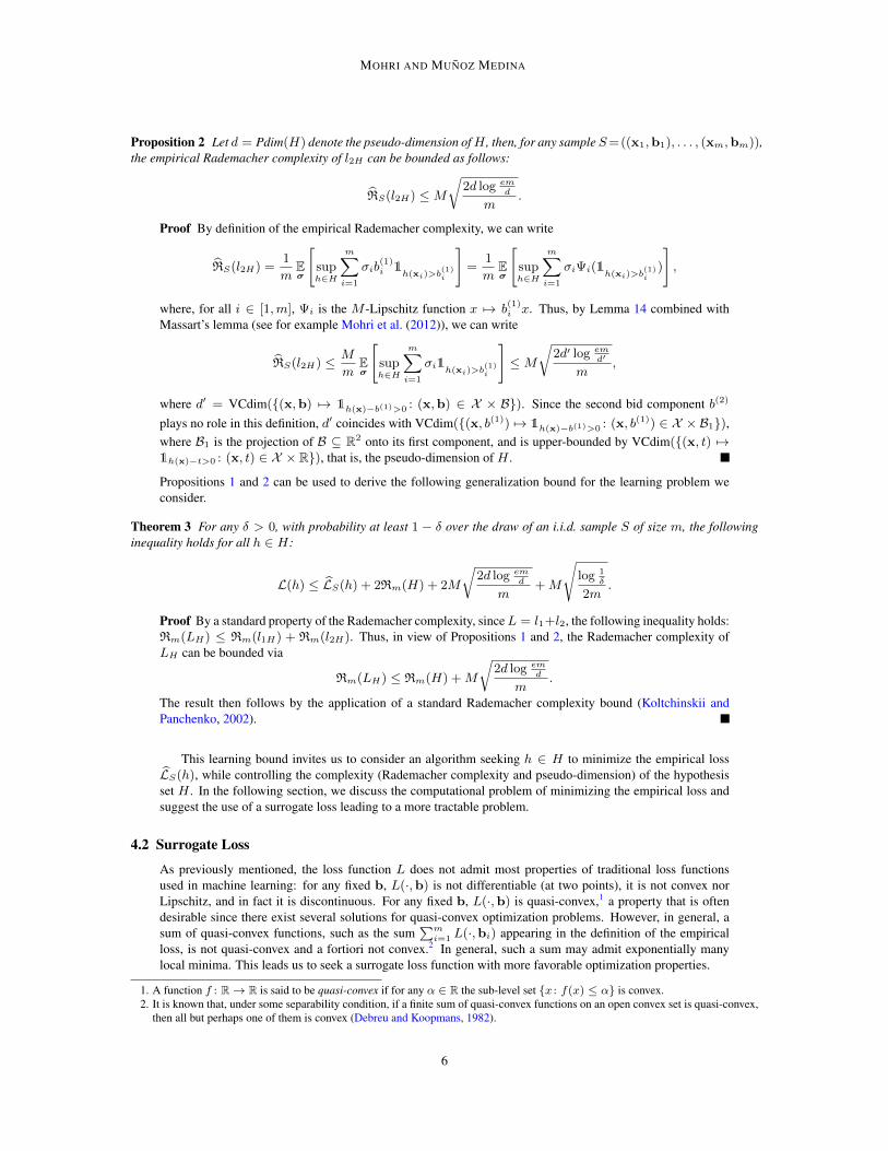
(a) (b)Figure 2: (a) Piecewise linear convex surrogate loss Lp. (b) Comparison of the sum of real losses∑m

i=1 L(·,bi) for m = 500 with the sum of convex surrogate losses. Note that the minimizersare significantly different.

A standard method in machine learning consists of replacing the loss function L with a convex upperbound (Bartlett et al., 2006). A natural candidate in our case is the piecewise linear function Lp shown inFigure 2(a). While this is a convex loss function, and thus convenient for optimization, it is not calibrated.That is, it is possible for rp ∈ argminEb[Lp(r,b)] to have a large expected true loss. Therefore, it does notprovide us with a useful surrogate. The calibration problem is illustrated by Figure 2(b) in dimension one,where the true objective function to be minimized

∑mi=1 L(r,bi) is compared with the sum of the surrogate

losses. The next theorem shows that this problem affects any non-constant convex surrogate. It is expressedin terms of the loss L : R×R+ → R defined by L(r, b) = −r1r≤b, which coincides with L when the secondbid is 0.

Definition 4 We say that a function Lc : [0,M ]× [0,M ]→ R is consistent with L if, for any distributionD, there existsa minimizer r∗ ∈ argminr Eb∼D[Lc(r, b)] such that r∗ ∈ argminr Eb∼D[L(r, b)].

Definition 5 We say that a sequence of functions (Ln)n∈N mapping [0,M ] × [0,M ] to R is weakly consistent with Lif there exists a sequence (rn)n∈N in R with rn ∈ argminr Eb∼D[Ln(r, b)] for all n ∈ N such that limn→+∞ rn = r∗

with r∗ ∈ argminEb∼D[L(r, b)].

Proposition 6 (Convex surrogates) Let Lc : [0,M ] × [0,M ] → R be a bounded function, convex with respect to itsfirst argument. If Lc is consistent with L, then Lc(·, b) is constant for any b ∈ [0,M ].

Proof The idea behind the proof is the following: for any two bids b1 < b2, there exists a distribution D withsupport {b1, b2} such that Eb∼D[L(r, b)] is minimized at both r = b1 and r = b2. We show this implies thatEb∼D[Lc(r, b)] must attain a minimum at both points too. By convexity of Lc, it follows that Eb∼D[Lc(r, b)]must be constant on the interval [b1, b2]. The main part of the proof will be showing that this implies thatthe function Lc(·, b1) must also be constant on the interval [b1, b2]. Finally, since the value of b2 was chosenarbitrarily, it will follow that Lc(·, b1) is constant.

Let 0 < b1 < b2 < M and, for any µ ∈ [0, 1], let Dµ denote the probability distribution with supportincluded in {b1, b2} defined byDµ(b1) = µ and let Eµ denote the expectation with respect to this distribution.A straightforward calculation shows that the unique minimizer of Eµ[L(r, b)] is given by b2 if µ > b2−b1

b2and

by b1 if µ < b2−b1b2

. Therefore, if Fµ(r) = Eµ[Lc(r, b)], it must be the case that b2 is a minimizer of Fµ forµ > b2−b1

b2and b1 is a minimizer of Fµ for µ < b2−b1

b2.

For a convex function f : R → R, we denote by f− its left-derivative and by f+ its right-derivative,which are guaranteed to exist. We will also denote here, for any b ∈ R, by g−(·, b) and g+(·, b) the left- andright-derivatives of the function g(·, b) and by g′(·, b) its derivative, when it exists. Recall that for a convexfunction f , if x0 is a minimizer, then f−(x0) ≤ 0 ≤ f+(x0). In view of that and the minimizing properties

7

MOHRI AND MUNOZ MEDINA

of b1 and b2, the following inequalities hold:

0 ≥ F−µ (b2) = µL−c (b2, b1) + (1− µ)L−c (b2, b2) for µ >b2 − b1b2

, (3)

0 ≤ F+µ (b1) ≤ F−µ (b2) for µ <

b2 − b1b2

, (4)

where the second inequality in (4) holds by convexity of Fµ and the fact that b1 < b2. By setting µ = b2−b1b2

,it follows from inequalities (3) and (4) that F−µ (b2) = 0 and F+

µ (b1) = 0. By convexity of Fµ, it follows thatFµ is constant on the interval (b1, b2). We now show this may only happen if Lc(·, b1) is also constant. Byrearranging terms in (3) and plugging in the expression of µ, we obtain the equivalent condition

(b2 − b1)L−c (b2, b1) = −b1L−c (b2, b2).

Since Lc is a bounded function, it follows that L−c (b2, b1) is bounded for any b1, b2 ∈ (0,M), therefore asb1 → b2 we must have b2L−c (b2, b2) = 0, which implies L−c (b2, b2) = 0 for all b2 > 0. In view of this,inequality (3) may only be satisfied if L−c (b2, b1) ≤ 0. However, the convexity of Lc implies L−c (b2, b1) ≥L−c (b1, b1) = 0. Therefore, L−c (b2, b1) = 0 must hold for all b2 > b1 > 0. Similarly, by definition of Fµ,the first inequality in (4) implies

µL+c (b1, b1) + (1− µ)L+

c (b1, b2) ≥ 0. (5)

Nevertheless, for any b2 > b1 we have 0 = L−c (b1, b1) ≤ L+c (b1, b1) ≤ L−c (b2, b1) = 0. Consequently,

L+c (b1, b1) = 0 for all b1 > 0. Furthermore, L+

c (b1, b2) ≤ L+c (b2, b2) = 0. Therefore, for inequality (5) to

be satisfied, we must have L+c (b1, b2) = 0 for all b1 < b2.

Thus far, we have shown that for any b > 0, if r ≥ b, then L−c (r, b) = 0, while L+c (r, b) = 0 for r ≤ b.

A simple convexity argument shows that Lc(·, b) is then differentiable and L′c(r, b) = 0 for all r ∈ (0,M),which in turn implies that Lc(·, b) is a constant function.

The result of the previous proposition can be considerably strengthened, as shown by the following theorem.As in the proof of the previous proposition, to simplify the notation, for any b ∈ R, we will denote by g′(·, b)the derivative of a differentiable function g(·, b).

Theorem 7 Let (Ln)n∈N denote a sequence of functions mapping [0,M ]×[0,M ] to R that are convex and differentiablewith respect to their first argument and satisfy the following conditions:

• supb∈[0,M ],n∈N max(|L′n(0, b)|, |L′n(M, b)| = K <∞;

• (Ln)n is weakly consistent with L;

• Ln(0, b) = 0 for all n ∈ N and for all b.

If the sequence (Ln)n converges pointwise to a function Lc, then Ln(·, b) converges uniformly to Lc(·, b) ≡ 0.

We defer the proof of this theorem to Appendix B and present here only a sketch of the proof. We first showthat the convexity of the functions Ln implies that the convergence to Lc must be uniform and that Lc isconvex with respect to its first argument. This fact and the weak consistency of the sequence Ln will thenimply that Lc is consistent with L and therefore must be constant by Proposition 6.

The theorem just presented shows that even a weakly consistent sequence of convex losses is uniformlyclose to a constant function and therefore not helpful to tackle the learning task we consider. This suggestssearching for surrogate losses that admit weaker regularity assumptions such as Lipschitz continuity.

Perhaps, the most natural surrogate loss function is then Lγ , an upper bound on L defined for all γ > 0by:

Lγ(r,b) = −b(2)1r≤b(2) − r1b(2)<r≤

((1−γ)b(1)

)∨b(2)

+(1− γ

γ∨ b(2)

b(1) − b(2)

)(r − b(1))1(

(1−γ)b(1))∨b(2)<r≤b(1)

,

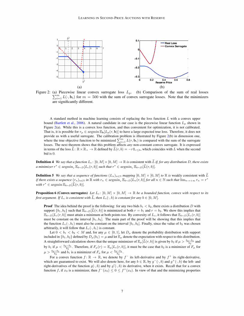
where c ∨ d = max(c, d). The plot of this function is shown in Figure 3(a). The max terms ensure that thefunction is well defined if (1−γ)b(1) < b(2). However, this turns out to be also a poor choice as Lγ is a loose

8

LEARNING IN SECOND-PRICE AUCTIONS WITH RESERVE

0 1 2 3 4 5

-4

-3

-2

-1

0

1b2 (1 ! !)b1

b1

0 1 2 3 4 5

-4

-3

-2

-1

0

1b2 (1 + !)b1

b1

(a) (b)

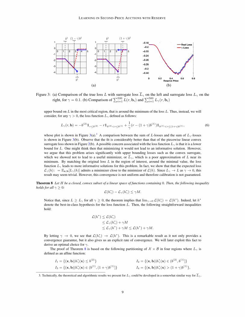
Figure 3: (a) Comparison of the true loss L with surrogate loss Lγ on the left and surrogate loss Lγ on theright, for γ = 0.1. (b) Comparison of

∑500i=1 L(r,bi) and

∑500i=1 Lγ(r,bi)

upper bound on L in the most critical region, that is around the minimum of the loss L. Thus, instead, we willconsider, for any γ > 0, the loss function Lγ defined as follows:

Lγ(r,b) = −b(2)1r≤b(2) − r1b(2)<r≤b(1) +

1

γ(r − (1 + γ)b(1))1b(1)<r≤(1+γ)b(1) , (6)

whose plot is shown in Figure 3(a).3 A comparison between the sum of L-losses and the sum of Lγ-lossesis shown in Figure 3(b). Observe that the fit is considerably better than that of the piecewise linear convexsurrogate loss shown in Figure 2(b). A possible concern associated with the loss functionLγ is that it is a lowerbound for L. One might think then that minimizing it would not lead to an informative solution. However,we argue that this problem arises significantly with upper bounding losses such as the convex surrogate,which we showed not to lead to a useful minimizer, or Lγ , which is a poor approximation of L near itsminimum. By matching the original loss L in the region of interest, around the minimal value, the lossfunction Lγ leads to more informative solutions for this problem. In fact, we show that that the expected lossLγ(h) : = Ex,b[Lγ(h)] admits a minimizer close to the minimizer of L(h). Since Lγ → L as γ → 0, thisresult may seem trivial. However, this convergence is not uniform and therefore calibration is not guaranteed.

Theorem 8 Let H be a closed, convex subset of a linear space of functions containing 0. Then, the following inequalityholds for all γ ≥ 0:

L(h∗γ)− Lγ(h∗γ) ≤ γM.

Notice that, since L ≥ Lγ for all γ ≥ 0, the theorem implies that limγ→0 L(h∗γ) = L(h∗). Indeed, let h∗

denote the best-in-class hypothesis for the loss function L. Then, the following straightforward inequalitieshold:

L(h∗) ≤ L(h∗γ)

≤ Lγ(h∗γ) + γM

≤ Lγ(h∗) + γM ≤ L(h∗) + γM.

By letting γ → 0, we see that L(h∗γ) → L(h∗). This is a remarkable result as it not only provides aconvergence guarantee, but it also gives us an explicit rate of convergence. We will later exploit this fact toderive an optimal choice for γ.

The proof of Theorem 8 is based on the following partitioning of X × B in four regions where Lγ isdefined as an affine function:

I1 = {(x,b)|h∗γ(x) ≤ b(2)} I2 = {(x,b)|h∗γ(x) ∈ (b(2), b(1)]}

I3 = {(x,b)|h∗γ(x) ∈ (b(1), (1 + γ)b(1)]} I4 = {(x,b)|h∗γ(x) > (1 + γ)b(1)},

3. Technically, the theoretical and algorithmic results we present for Lγ could be developed in a somewhat similar way for Lγ .

9

MOHRI AND MUNOZ MEDINA

Notice that Lγ and L differ only on I3. Therefore, we only need to bound the measure of this set which canbe done as in Lemma 15 (see Appendix C).Proof [Theorem 8]. We can express the difference as

Ex,b

[L(h∗γ(x),b)− Lγ(h∗γ(x),b)

]=

4∑k=1

Ex,b

[(L(h∗γ(x),b)− Lγ(h∗γ(x),b))1Ik (x,b)

]= E

x,b

[(L(h∗γ(x),b)− Lγ(h∗γ(x),b))1I3(x,b)

]= E

x,b

[ 1

γ((1 + γ)b(1) − h∗γ(x))1I3(x,b))

]. (7)

Furthermore, for (x,b) ∈ I3, we know that b(1) < h∗γ(x). Thus, we can bound (7) by Ex,b[h∗γ(x)1I3(x,b)],

which, by Lemma 15 in Appendix C, is upper bounded by γ Ex,b

[h∗γ(x)1I2(x,b)

]. Thus, the following

inequalities hold:

Ex,b

[L(h∗γ(x),b)

]− E

x,b

[Lγ(h∗γ(x),b)

]≤ γ E

x,b

[h∗γ(x)1I2(x,b)

]≤ γ E

x,b

[b(1)

1I2(x,b)]≤ γM,

using the fact that h∗γ(x) ≤ b(1) for (x,b) ∈ I2.

The 1/γ-Lipschitzness of Lγ can be used to prove the following generalization bound.

Theorem 9 Fix γ ∈ (0, 1] and let S denote a sample of size m. Then, for any δ > 0, with probability at least 1− δ overthe choice of the sample S, for all h ∈ H , the following holds:

Lγ(h) ≤ Lγ(h) +2

γRm(H) +M

√log 1

δ

2m. (8)

Proof Let Lγ,H denote the family of functions {(x,b)→ Lγ(h(x), b) : h ∈ H}. The loss function Lγ is 1γ

-Lipschitz since the slope of the lines defining it is at most 1

γ. Thus, using the contraction lemma (Lemma 14)

as in the proof of Proposition 1, gives Rm(Lγ,H) ≤ 1γRm(H). The application of a standard Rademacher

complexity bound to the family of functions Lγ,H then shows that for any δ > 0, with probability at least1− δ, for any h ∈ H , the following holds:

Lγ(h) ≤ Lγ(h) +2

γRm(H) +M

√log 1

δ

2m.

We conclude this section by showing that Lγ admits a stronger form of consistency. More precisely, we provethat the generalization error of the best-in-class hypothesis L∗ := L(h∗) can be lower bounded in terms ofthat of the empirical minimizer of Lγ , hγ : = argminh∈H Lγ(h).

Theorem 10 Let M = supb∈B b(1) and let H be a hypothesis set with pseudo-dimension d = Pdim(H). Then, for any

δ > 0 and a fixed value of γ > 0, with probability at least 1 − δ over the choice of a sample S of size m, the followinginequality holds:

L∗ ≤ L(hγ) ≤ L∗ +2γ + 2

γRm(H) + γM + 2M

√2d log εm

d

m+ 2M

√log 2

δ

2m.

Proof By Theorem 3, with probability at least 1− δ/2, the following holds:

L(hγ) ≤ LS(hγ) + 2Rm(H) + 2M

√2d log εm

d

m+M

√log 2

δ

2m. (9)

10

LEARNING IN SECOND-PRICE AUCTIONS WITH RESERVE

−a(1)

b(2)

−a(2)r

b(1)

a(3)r − a(4)

(1 + η)b(1) b(2)i b

(1)i

nk nk+1

(1 + η)b(1)i

Vi(nk,bi) = −a(2)i nk

Vi(nk+1,bi) = −a(2)i nk+1

(a) (b)

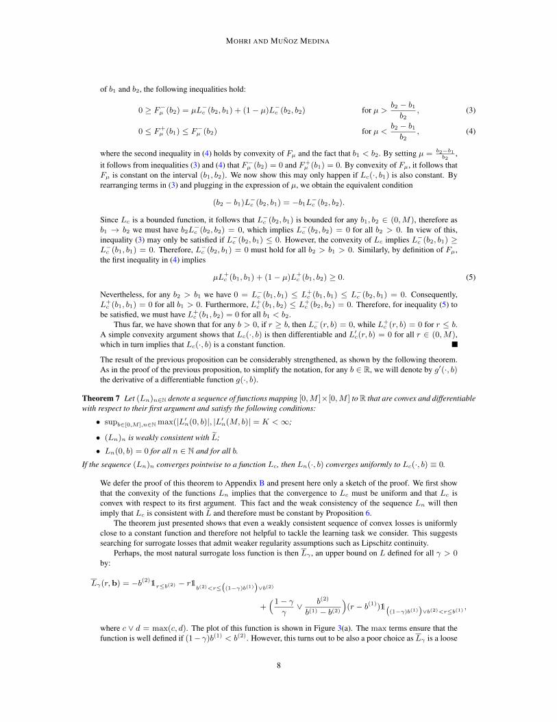
Figure 4: (a) Prototypical v-function. (b) Illustration of the fact that the definition of Vi(r,bi) does notchange on an interval [nk, nk+1].

Applying Lemma 15 with the empirical distribution induced by the sample, we can bound LS(hγ) byLγ(hγ) + γM . The first term of the previous expression is less than Lγ(h∗γ) by definition of hγ . More-over, the same analysis used in the proof of Theorem 9 shows that with probability 1− δ/2,

Lγ(h∗γ) ≤ Lγ(h∗γ) +2

γRm(H) +M

√log 2

δ

2m.

Finally, by definition of h∗γ and using the fact that L is an upper bound on Lγ , we can write Lγ(h∗γ) ≤Lγ(h∗) ≤ L(h∗). Thus,

LS(hγ) ≤ L(h∗) +2

γRm(H) +M

√log 2

δ

2m+ γM.

Replacing this inequality in (9) and applying the union bound yields the result.

This bound can be extended to hold uniformly over all γ at the price of a term in O(√

log log21γ√

m

). Thus, for

appropriate choices of γ as a function of m (for instance γ = 1/m1/4) we can guarantee the convergence ofL(hγ) to L∗, a stronger form of consistency (See Appendix C).

These results are reminiscent of the standard margin bounds with γ playing the role of a margin. Thesituation here is however somewhat different. Our learning bounds suggest, for a fixed γ ∈ (0, 1], to seeka hypothesis h minimizing the empirical loss Lγ(h) while controlling a complexity term upper boundingRm(H), which in the case of a family of linear hypotheses could be ‖h‖2K for some PSD kernel K. Sincethe bound can hold uniformly for all γ, we can use it to select γ out of a finite set of possible grid searchvalues. Alternatively, γ can be set via cross-validation. In the next section, we present algorithms for solvingthis regularized empirical risk minimization problem.

5. AlgorithmsIn this section, we show how to minimize the empirical risk under two regimes: first we analyze the no-featurescenario considered in Cesa-Bianchi et al. (2013) and then we present an algorithm to solve the more generalfeature-based revenue optimization problem.

5.1 No-Feature Case

We now present a general algorithm to optimize sums of functions similar to Lγ or L in the one-dimensionalcase.

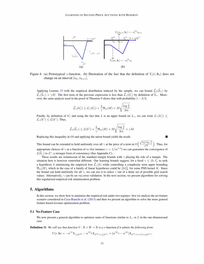
Definition 11 We will say that function V : R× B → R is a v-function if it admits the following form:

V (r,b) = −a(1)1r≤b(2) − a

(2)r1b(2)<r≤b(1) + (a(3)r − a(4))1b(1)<r<(1+η)b(1) ,

11

MOHRI AND MUNOZ MEDINA

with a(1) > 0 and η > 0 constants and a(2), a(3), a(4) defined by a(1) = ηa(3)b(2), a(2) = ηa(3), and a(4) =a(3)(1 + η)b(1).

Figure 4(a) illustrates this family of loss functions. A v-function is a generalization of Lγ and L. Indeed, anyv-function V satisfies V (r,b) ≤ 0 and attains its minimum at b(1). Finally, as can be seen straightforwardlyfrom Figure 3, Lγ is a v-function for any γ > 0. We consider the following general problem of minimizing asum of v-functions:

minr≥0

F (r) :=

m∑i=1

Vi(r,bi). (10)

Observe that this is not a trivial problem since, for any fixed bi, Vi(·,bi) is non-convex and that, in general,a sum of m such functions may admit many local minima. Of course, we can seek a solution that is ε-close tothe optimal reserve via a grid search over points ri = iε. However, the guarantees for that algorithm woulddepend on the continuity of the function. In particular, this algorithm might fail for the loss L. Instead, weexploit the particular structure of a v-function to exactly minimize F . The following proposition, which isproven in Appendix D, shows that the minimum is attained at one of the highest bids, which matches theintuition. Notice that for the loss function L this is immediate since if r is not a highest bid, one can raise thereserve price without increasing any of the component losses.

Proposition 12 Problem (10) admits a solution r∗ that satisfies r∗ = b(1)i for some i ∈ [1,m].

Problem (10) can thus be reduced to examining the value of the function for the m arguments b(1)i ,

i ∈ [1,m]. This yields a straightforward method for solving the optimization which consists of comput-ing F (b

(1)i ) for all i and taking the minimum. But, since the computation of each F (b

(1)i ) takes O(m), the

overall computational cost is in O(m2), which can be prohibitive for even moderately large values of m.Instead, we present a combinatorial algorithm to solve the optimization problem (10) in O(m logm). Let

N =⋃i{b

(1)i , b

(2)i , (1 + η)b

(1)i } denote the set of all boundary points associated with the functions V (·,bi).

The algorithm proceeds as follows: first, sort the set N to obtain the ordered sequence (n1, . . . , n3m), whichcan be achieved in O(m logm) using a comparison-based sorting algorithm. Next, evaluate F (n1) and com-pute F (nk+1) from F (nk) for all k.

The main idea of the algorithm is the following: since the definition of Vi(·, bi) can only change atboundary points (see also Figure 4(b)), computing F (nk+1) from F (nk) can be achieved in constant time.Indeed, since between nk and nk+1 there are only two boundary points, we can compute V (nk+1,bi) fromV (nk,bi) by calculating V for only two values of bi, which can be done in constant time. We now give amore detailed description and proof of correctness of our algorithm.

Proposition 13 There exists an algorithm to solve the optimization problem (10) in O(m logm).

Proof The pseudocode of the algorithm is given in Algorithm 1, where a(1)i , ..., a

(4)i denote the parameters

defining the functions Vi(r,bi). We will prove that, after running Algorithm 1, we can compute F (nj) inconstant time using:

F (nj) = c(1)j + c

(2)j nj + c

(3)j nj + c

(4)j . (11)

This holds trivially for n1 since by definition n1 ≤ b(2)i for all i and therefore F (n1) = −

∑mi=1 a

(1)i . Now,

assume that (11) holds for j, we prove that it must also hold for j + 1. Suppose nj = b(2)i for some i (the

cases nj = b(1)i and nj = (1 + η)b

(1)i can be handled in the same way). Then Vi(nj ,bi) = −a(1)

i and wecan write ∑

k 6=i

Vk(nj ,bk) = F (nj)− V (nj ,bi) = (c(1)j + c

(2)j nj + c

(3)j nj + c

(4)j ) + a

(1)i .

Thus, by construction we would have:

c(1)j+1 + c

(2)j+1nj+1 + c

(3)j+1nj+1 + c

(4)j+1 = c

(1)j + a

(1)i + (c

(2)j − a

(2)i )nj+1 + c

(3)j nj+1 + c

(4)j

= (c(1)j + c

(2)j nj+1 + c

(3)j nj+1 + c

(4)j ) + a

(1)i − a

(2)i nj+1

=∑k 6=i

Vk(nj+1,bk)− a(2)i nj+1,

12

LEARNING IN SECOND-PRICE AUCTIONS WITH RESERVE

Algorithm 1 Sorting

N :=⋃mi=1{b

(1)i , b

(2)i , (1 + η)b

(1)i };

n1, ..., n3m) = Sort(N );Set ci := (c

(1)i , c

(2)i , c

(3)i , c

(4)i ) = 0 for i = 1, ..., 3m;

Set c(1)1 = −∑m

i=1 a(1)i ;

for j = 2, ..., 3m doSet cj = cj−1;if nj−1 = b

(2)i for some i then

c(1)j = c

(1)j + a

(1)i ;

c(2)j = c

(2)j − a

(2)i ;

else if nj−1 = b(1)i for some i then

c(2)j = c

(2)j + a

(2)i ;

c(3)j = c

(3)j + a

(3)i ;

c(4)j = c

(4)j − a

(4)i ;

elsec(3)j = c

(3)j − a

(3)i ;

c(4)j = c

(4)j + a

(4)i ;

end ifend for

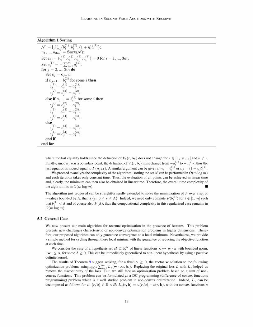
where the last equality holds since the definition of Vk(r,bk) does not change for r ∈ [nj , nj+1] and k 6= i.Finally, since nj was a boundary point, the definition of Vi(r,bi) must change from−a(1)

i to−a(2)i r, thus the

last equation is indeed equal to F (nj+1). A similar argument can be given if nj = b(1)i or nj = (1 + η)b

(1)i .

We proceed to analyze the complexity of the algorithm: sorting the setN can be performed inO(m logm)and each iteration takes only constant time. Thus, the evaluation of all points can be achieved in linear timeand, clearly, the minimum can then also be obtained in linear time. Therefore, the overall time complexity ofthe algorithm is in O(m logm).

The algorithm just proposed can be straightforwardly extended to solve the minimization of F over a set ofr-values bounded by Λ, that is {r : 0 ≤ r ≤ Λ}. Indeed, we need only compute F (b

(1)i ) for i ∈ [1,m] such

that b(1)i < Λ and of course also F (Λ), thus the computational complexity in this regularized case remains in

O(m logm).

5.2 General Case

We now present our main algorithm for revenue optimization in the presence of features. This problempresents new challenges characteristic of non-convex optimization problems in higher dimensions. There-fore, our proposed algorithm can only guarantee convergence to a local minimum. Nevertheless, we providea simple method for cycling through these local minima with the guarantee of reducing the objective functionat each time.

We consider the case of a hypothesis set H ⊂ RN of linear functions x 7→ w · x with bounded norm,‖w‖ ≤ Λ, for some Λ ≥ 0. This can be immediately generalized to non-linear hypotheses by using a positivedefinite kernel.

The results of Theorem 9 suggest seeking, for a fixed γ ≥ 0, the vector w solution to the followingoptimization problem: min‖w‖≤Λ

∑mi=1 Lγ(w · xi,bi). Replacing the original loss L with Lγ helped us

remove the discontinuity of the loss. But, we still face an optimization problem based on a sum of non-convex functions. This problem can be formulated as a DC-programming (difference of convex functionsprogramming) problem which is a well studied problem in non-convex optimization. Indeed, Lγ can bedecomposed as follows for all (r,b) ∈ R × B: Lγ(r,b) = u(r,b) − v(r,b), with the convex functions u

13

MOHRI AND MUNOZ MEDINA

and v defined by

u(r,b) = −r1r<b(1) + r−(1+γ)b(1)

γ1r≥b(1)

v(r,b) = (−r + b(2))1r<b(2) + r−(1+γ)b(1)

γ1r>(1+γ)b(1) .

Using the decomposition Lγ = u− v, our optimization problem can be formulated as follows:

minw∈RN

U(w)− V (w) subject to ‖w‖ ≤ Λ, (12)

where U(w) =∑mi=1 u(w ·xi,bi) and V (w) =

∑mi=1 v(w ·xi,bi), which shows that it can be formulated

as a DC-programming problem. The global minimum of the optimization problem (12) can be found using acutting plane method (Horst and Thoai, 1999), but that method only converges in the limit and does not admitknown algorithmic convergence guarantees.4 There exists also a branch-and-bound algorithm with exponentialconvergence for DC-programming (Horst and Thoai, 1999) for finding the global minimum. Nevertheless, in(Tao and An, 1997), it is pointed out that such combinatorial algorithms fail to solve real-world DC-programsin high dimensions. In fact, our implementation of this algorithm shows that the convergence of the algorithmin practice is extremely slow for even moderately high-dimensional problems. Another attractive solution forfinding the global solution of a DC-programming problem over a polyhedral convex set is the combinatorialsolution of Tuy (1964). However, this method requires explicitly specifying the slope and offsets for thepiecewise linear function corresponding to a sum of Lγ losses and incurs an exponential cost in time andspace.

An alternative consists of using the DC algorithm (DCA), a primal-dual sub-differential method of DinhTao and Hoai An Tao and An (1998), (see also Tao and An (1997) for a good survey). This algorithm isapplicable when u and v are proper lower semi-continuous convex functions as in our case. When v isdifferentiable, the DC algorithm coincides with the CCCP algorithm of Yuille and Rangarajan (2003), whichhas been used in several contexts in machine learning and analyzed by Sriperumbudur and Lanckriet (2012).

The general proof of convergence of the DC algorithm was given by Tao and An (1998). In some specialcases, the DC algorithm can be used to find the global minimum of the problem as in the trust region problem(Tao and An, 1998), but, in general, the DC algorithm or its special case CCCP are only guaranteed to convergeto a critical point (Tao and An, 1998; Sriperumbudur and Lanckriet, 2012). Nevertheless, the number ofiterations of the DC algorithm is relatively small. Its convergence has been shown to be in fact linear forDC-programming problems such as ours (Yen et al., 2012). The algorithm we are proposing goes one stepfurther than that of Tao and An (1998): we use DCA to find a local minimum but then restart our algorithmwith a new seed that is guaranteed to reduce the objective function. Unfortunately, we are not in the sameregime as in the trust region problem of Tao and An (1998) where the number of local minima is linear in thesize of the input. Indeed, here, the number of local minima can be exponential in the number of dimensionsof the feature space and it is not clear to us how the combinatorial structure of the problem could help us ruleout some local minima faster and make the optimization more tractable.

In the following, we describe more in detail the solution we propose for solving the DC-programmingproblem (12). The functions v and V are not differentiable in our context but they admit a sub-gradientat all points. We will denote by δV (w) an arbitrary element of the sub-gradient ∂V (w), which coincideswith ∇V (w) at points w where V is differentiable. The DC algorithm then coincides with CCCP, modulothe replacement of the gradient of V by δV (w). It consists of starting with a weight vector w0 ≤ Λ andof iteratively solving a sequence of convex optimization problems obtained by replacing V with its linearapproximation giving wt as a function of wt−1, for t = 1, . . . , T : wt ∈ argmin‖w‖≤Λ U(w)−δV (wt−1) ·w. This problem can be rewritten in our context as the following:

min‖w‖2≤Λ2,s

m∑i=1

si − δV (wt−1) ·w (13)

subject to (si≥−w · xi)∧[si≥

1

γ

(w · xi−(1 + γ)b

(1)i

)].

4. Some claims of Horst and Thoai (1999), e.g., Proposition 4.4 used in support of the cutting plane algorithm, are incorrect (Tuy,2002).

14

LEARNING IN SECOND-PRICE AUCTIONS WITH RESERVE

DC Algorithmw← w0 . initializationwhile v 6= w dov← DCA(w) . DC algorithmu← v

‖v‖η∗ ← min0≤η≤Λ

∑u·xi>0 Lγ(ηu · xi,bi)

w← η∗vend while

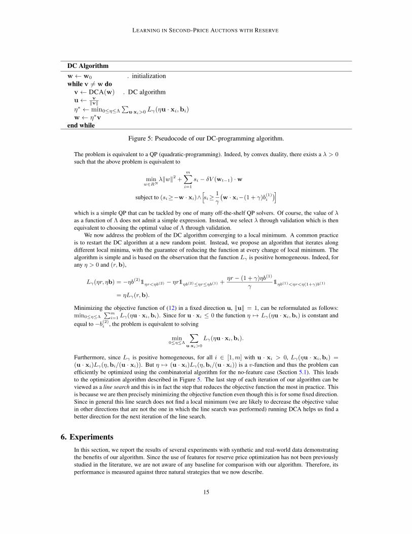
Figure 5: Pseudocode of our DC-programming algorithm.

The problem is equivalent to a QP (quadratic-programming). Indeed, by convex duality, there exists a λ > 0such that the above problem is equivalent to

minw∈RN

λ‖w‖2 +

m∑i=1

si − δV (wt−1) ·w

subject to (si≥−w · xi)∧[si≥

1

γ

(w · xi−(1 + γ)b

(1)i

)]which is a simple QP that can be tackled by one of many off-the-shelf QP solvers. Of course, the value of λas a function of Λ does not admit a simple expression. Instead, we select λ through validation which is thenequivalent to choosing the optimal value of Λ through validation.

We now address the problem of the DC algorithm converging to a local minimum. A common practiceis to restart the DC algorithm at a new random point. Instead, we propose an algorithm that iterates alongdifferent local minima, with the guarantee of reducing the function at every change of local minimum. Thealgorithm is simple and is based on the observation that the function Lγ is positive homogeneous. Indeed, forany η > 0 and (r,b),

Lγ(ηr, ηb) = −ηb(2)1ηr<ηb(2) − ηr1ηb(2)≤ηr≤ηb(1) +

ηr − (1 + γ)ηb(1)

γ1ηb(1)<ηr<η(1+γ)b(1)

= ηLγ(r,b).

Minimizing the objective function of (12) in a fixed direction u, ‖u‖ = 1, can be reformulated as follows:min0≤η≤Λ

∑mi=1 Lγ(ηu · xi,bi). Since for u · xi ≤ 0 the function η 7→ Lγ(ηu · xi,bi) is constant and

equal to −b(2)i , the problem is equivalent to solving

min0≤η≤Λ

∑u·xi>0

Lγ(ηu · xi,bi).

Furthermore, since Lγ is positive homogeneous, for all i ∈ [1,m] with u · xi > 0, Lγ(ηu · xi,bi) =(u · xi)Lγ(η,bi/(u · xi)). But η 7→ (u · xi)Lγ(η,bi/(u · xi)) is a v-function and thus the problem canefficiently be optimized using the combinatorial algorithm for the no-feature case (Section 5.1). This leadsto the optimization algorithm described in Figure 5. The last step of each iteration of our algorithm can beviewed as a line search and this is in fact the step that reduces the objective function the most in practice. Thisis because we are then precisely minimizing the objective function even though this is for some fixed direction.Since in general this line search does not find a local minimum (we are likely to decrease the objective valuein other directions that are not the one in which the line search was performed) running DCA helps us find abetter direction for the next iteration of the line search.

6. ExperimentsIn this section, we report the results of several experiments with synthetic and real-world data demonstratingthe benefits of our algorithm. Since the use of features for reserve price optimization has not been previouslystudied in the literature, we are not aware of any baseline for comparison with our algorithm. Therefore, itsperformance is measured against three natural strategies that we now describe.

15

MOHRI AND MUNOZ MEDINA

As mentioned before, a standard solution for solving this problem would be the use of a convex surrogateloss. In view of that, we compare against the solution of the regularized empirical risk minimization of theconvex surrogate loss Lα shown in Figure 2(a) parametrized by α ∈ [0, 1] and defined by

Lα(r,b)=

{−r if r < b(1) + α(b(2) − b(1))(

(1−α)b(1)+αb(2)

α(b(1)−b(2))

)(r − b(1)) otherwise.

A second alternative consists of using ridge regression to estimate the first bid and of using its prediction asthe reserve price. A third algorithm consists of minimizing the loss while ignoring the feature vectors xi, i.e.,solving the problem minr≤Λ

∑ni=1 L(r,bi). It is worth mentioning that this third approach is very similar

to what advertisement exchanges currently use to suggest reserve prices to publishers. By using the empiricalversion of equation (2), we see that this algorithm is equivalent to finding the empirical distribution of bidsand optimizing the expected revenue with respect to this empirical distribution as in (Ostrovsky and Schwarz,2011) and (Cesa-Bianchi et al., 2013).

6.1 Artificial Data Sets

We generated 4 different synthetic data sets with different correlation levels between features and bids. Forall our experiments, the feature vectors x ∈ R21 were generated in as follows: x ∈ R20 was sampledfrom a standard Gaussian distribution and x = (x, 1) was created by adding an offset feature. We nowdescribe the bid generating process for each of the experiments as a function of the feature vector x. Forour first three experiments, shown in Figure 6(a)-(c), the highest bid and second highest bid were set tomax

(∣∣∣∑21i=1 xi

∣∣∣ + ε1,∣∣∣∑21

i=1xi2

∣∣∣ + ε2)

+and min

(∣∣∣∑21i=1 xi

∣∣∣ + ε1,∣∣∣∑21

i=1xi2

∣∣∣ + ε2)

+respectively,

where εi is a Gaussian random variable with mean 0. The standard deviation of the Gaussian noise was variedover the set {0, 0.25, 0.5}.

For our last artificial experiment, we used a generative model motivated by previous empirical observa-tions (Ostrovsky and Schwarz, 2011; Lahaie and Pennock, 2007): bids were generated by sampling two valuesfrom a log-normal distribution with means x ·w and x·w

2and standard deviation 0.5, with w a random vector

sampled from a standard Gaussian distribution.For all our experiments, the parameters λ, γ and α were selected respectively from the sets {2i|i ∈

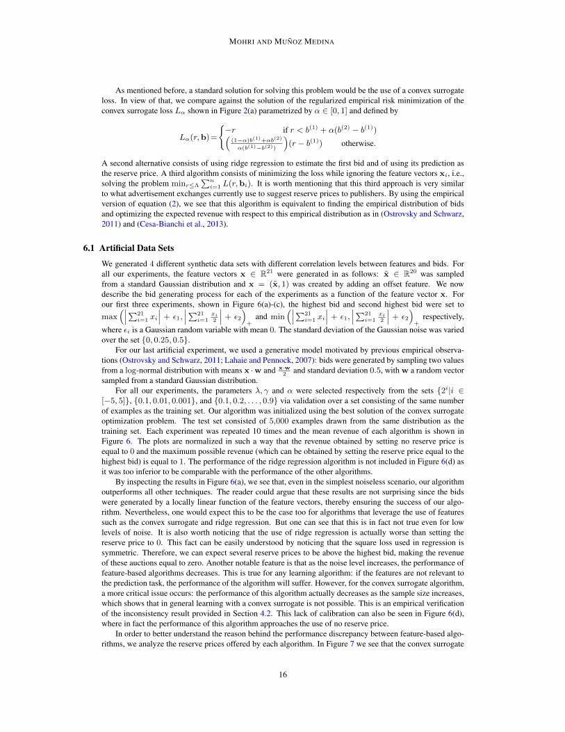
[−5, 5]}, {0.1, 0.01, 0.001}, and {0.1, 0.2, . . . , 0.9} via validation over a set consisting of the same numberof examples as the training set. Our algorithm was initialized using the best solution of the convex surrogateoptimization problem. The test set consisted of 5,000 examples drawn from the same distribution as thetraining set. Each experiment was repeated 10 times and the mean revenue of each algorithm is shown inFigure 6. The plots are normalized in such a way that the revenue obtained by setting no reserve price isequal to 0 and the maximum possible revenue (which can be obtained by setting the reserve price equal to thehighest bid) is equal to 1. The performance of the ridge regression algorithm is not included in Figure 6(d) asit was too inferior to be comparable with the performance of the other algorithms.

By inspecting the results in Figure 6(a), we see that, even in the simplest noiseless scenario, our algorithmoutperforms all other techniques. The reader could argue that these results are not surprising since the bidswere generated by a locally linear function of the feature vectors, thereby ensuring the success of our algo-rithm. Nevertheless, one would expect this to be the case too for algorithms that leverage the use of featuressuch as the convex surrogate and ridge regression. But one can see that this is in fact not true even for lowlevels of noise. It is also worth noticing that the use of ridge regression is actually worse than setting thereserve price to 0. This fact can be easily understood by noticing that the square loss used in regression issymmetric. Therefore, we can expect several reserve prices to be above the highest bid, making the revenueof these auctions equal to zero. Another notable feature is that as the noise level increases, the performance offeature-based algorithms decreases. This is true for any learning algorithm: if the features are not relevant tothe prediction task, the performance of the algorithm will suffer. However, for the convex surrogate algorithm,a more critical issue occurs: the performance of this algorithm actually decreases as the sample size increases,which shows that in general learning with a convex surrogate is not possible. This is an empirical verificationof the inconsistency result provided in Section 4.2. This lack of calibration can also be seen in Figure 6(d),where in fact the performance of this algorithm approaches the use of no reserve price.

In order to better understand the reason behind the performance discrepancy between feature-based algo-rithms, we analyze the reserve prices offered by each algorithm. In Figure 7 we see that the convex surrogate

16

LEARNING IN SECOND-PRICE AUCTIONS WITH RESERVE

(a)

-0.2-0.1

0 0.1 0.2 0.3 0.4 0.5 0.6 0.7

100 200 400 800 1600

Rev

enu

e

Sample size

NF CVX DC Reg

(b)

-0.2

-0.1

0

0.1

0.2

0.3

0.4

0.5

100 200 400 800 1600

Rev

enu

e

Sample size

NF CVX DC Reg

(c)-0.15

-0.1-0.05

0 0.05

0.1 0.15

0.2 0.25

0.3 0.35

0.4

100 200 400 800 1600

NF CVX DC Reg

(d)

-0.2-0.15

-0.1-0.05

0 0.05

0.1 0.15

0.2

200 300 400 600 800 1000120016002400

Rev

enu

e

Sample size

DC CVX NF

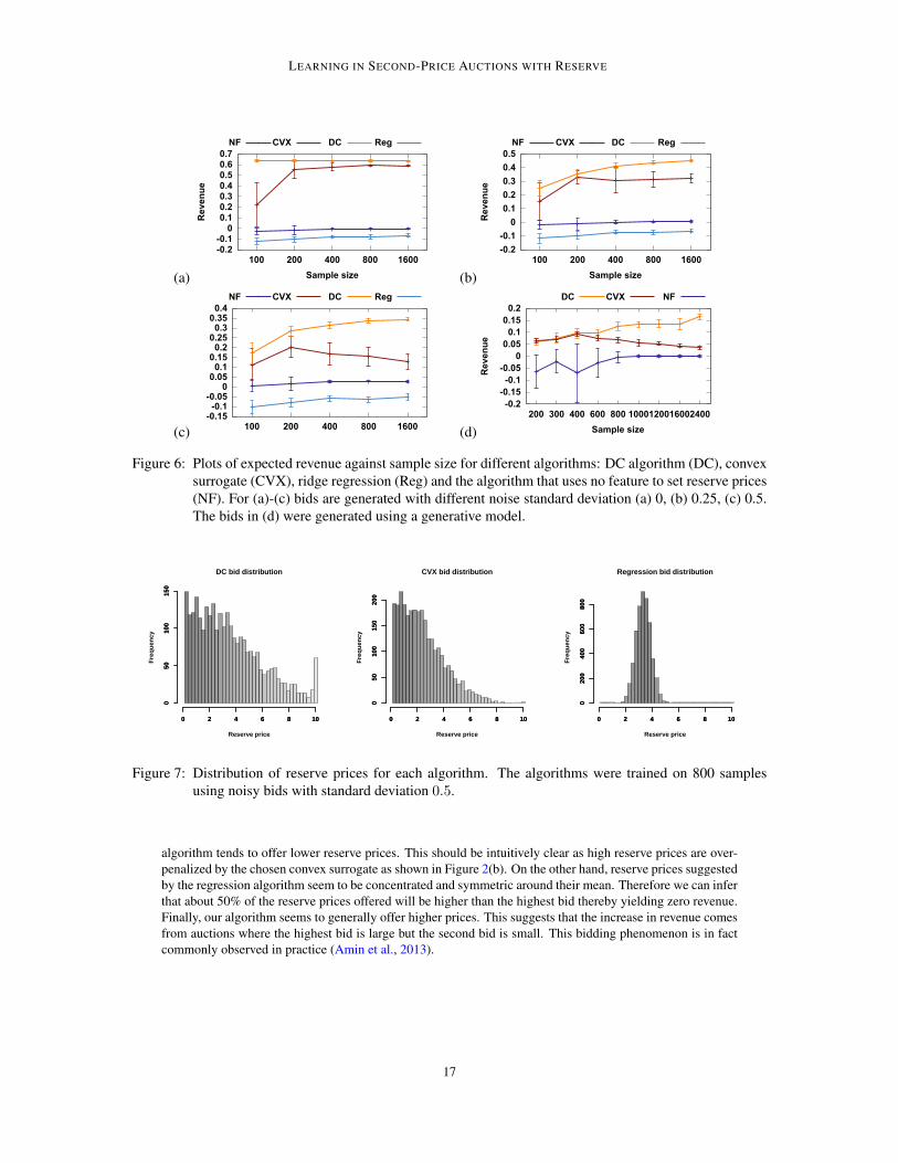
Figure 6: Plots of expected revenue against sample size for different algorithms: DC algorithm (DC), convexsurrogate (CVX), ridge regression (Reg) and the algorithm that uses no feature to set reserve prices(NF). For (a)-(c) bids are generated with different noise standard deviation (a) 0, (b) 0.25, (c) 0.5.The bids in (d) were generated using a generative model.

0 2 4 6 8 10

050

100

150

050

100

150

0 2 4 6 8 10

Reserve price

Fre

quen

cy

DC bid distribution

0 2 4 6 8 10

050

100

150

200

050

100

150

200

0 2 4 6 8 10

Reserve price

Fre

quen

cy

CVX bid distribution

0 2 4 6 8 10

020

040

060

080

00

200

400

600

800

0 2 4 6 8 10

Reserve price

Fre

quen

cyRegression bid distribution

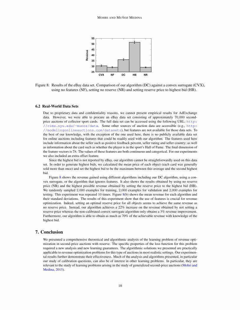
Figure 7: Distribution of reserve prices for each algorithm. The algorithms were trained on 800 samplesusing noisy bids with standard deviation 0.5.

algorithm tends to offer lower reserve prices. This should be intuitively clear as high reserve prices are over-penalized by the chosen convex surrogate as shown in Figure 2(b). On the other hand, reserve prices suggestedby the regression algorithm seem to be concentrated and symmetric around their mean. Therefore we can inferthat about 50% of the reserve prices offered will be higher than the highest bid thereby yielding zero revenue.Finally, our algorithm seems to generally offer higher prices. This suggests that the increase in revenue comesfrom auctions where the highest bid is large but the second bid is small. This bidding phenomenon is in factcommonly observed in practice (Amin et al., 2013).

17

MOHRI AND MUNOZ MEDINA

25

30

35

40

45

50

55

CVX NF DC HB NR

Rev

enu

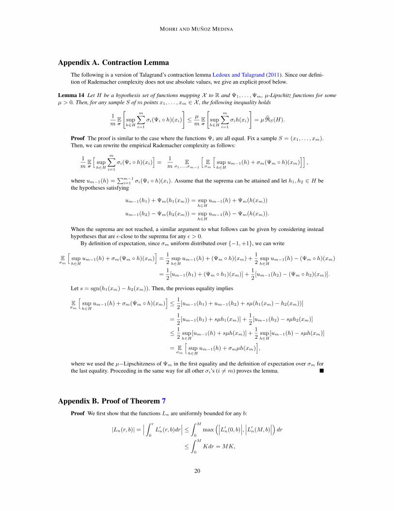
eFigure 8: Results of the eBay data set. Comparison of our algorithm (DC) against a convex surrogate (CVX),

using no features (NF), setting no reserve (NR) and setting reserve price to highest bid (HB).

6.2 Real-World Data Sets

Due to proprietary data and confidentiality reasons, we cannot present empirical results for AdExchangedata. However, we were able to procure an eBay data set consisting of approximately 70,000 second-price auctions of collector sport cards. The full data set can be accessed using the following URL: http://cims.nyu.edu/˜munoz/data. Some other sources of auction data are accessible (e.g., http://modelingonlineauctions.com/datasets), but features are not available for those data sets. Tothe best of our knowledge, with the exception of the one used here, there is no publicly available data setfor online auctions including features that could be readily used with our algorithm. The features used hereinclude information about the seller such as positive feedback percent, seller rating and seller country; as wellas information about the card such as whether the player is in the sport’s Hall of Fame. The final dimension ofthe feature vectors is 78. The values of these features are both continuous and categorical. For our experimentswe also included an extra offset feature.

Since the highest bid is not reported by eBay, our algorithm cannot be straightforwardly used on this dataset. In order to generate highest bids, we calculated the mean price of each object (each card was generallysold more than once) and set the highest bid to be the maximum between this average and the second highestbid.

Figure 8 shows the revenue gained using different algorithms including our DC algorithm, using a con-vex surrogate, or the algorithm that ignores features. It also shows the results obtained by using no reserveprice (NR) and the highest possible revenue obtained by setting the reserve price to the highest bid (HB).We randomly sampled 2,000 examples for training, 2,000 examples for validation and 2,000 examples fortesting. This experiment was repeated 10 times. Figure 8(b) shows the mean revenue for each algorithm andtheir standard deviations. The results of this experiment show that the use of features is crucial for revenueoptimization. Indeed, setting an optimal reserve price for all objects seems to achieve the same revenue asno reserve price. Instead, our algorithm achieves a 22% increase on the revenue obtained by not setting areserve price whereas the non-calibrated convex surrogate algorithm only obtains a 3% revenue improvement.Furthermore, our algorithm is able to obtain as much as 70% of the achievable revenue with knowledge of thehighest bid.

7. ConclusionWe presented a comprehensive theoretical and algorithmic analysis of the learning problem of revenue opti-mization in second-price auctions with reserve. The specific properties of the loss function for this problemrequired a new analysis and new learning guarantees. The algorithmic solutions we presented are practicallyapplicable to revenue optimization problems for this type of auctions in most realistic settings. Our experimen-tal results further demonstrate their effectiveness. Much of the analysis and algorithms presented, in particularour study of calibration questions, can also be of interest in other learning problems. In particular, they arerelevant to the study of learning problems arising in the study of generalized second-price auctions (Mohri andMedina, 2015).

18

LEARNING IN SECOND-PRICE AUCTIONS WITH RESERVE

AcknowledgmentsWe thank Afshin Rostamizadeh and Umar Syed for several discussions about the topic of this work and ICMLand JMLR reviewers for useful comments. We also warmly thank Jay Grossman for providing us access tothe eBay data set used in this paper. Finally, we thank Le Thi Hoai An for extensive discussions on DCprogramming. This work was partly funded by the NSF award IIS-1117591.

19

MOHRI AND MUNOZ MEDINA

Appendix A. Contraction LemmaThe following is a version of Talagrand’s contraction lemma Ledoux and Talagrand (2011). Since our defini-tion of Rademacher complexity does not use absolute values, we give an explicit proof below.

Lemma 14 Let H be a hypothesis set of functions mapping X to R and Ψ1, . . . ,Ψm, µ-Lipschitz functions for someµ > 0. Then, for any sample S of m points x1, . . . , xm ∈ X , the following inequality holds

1

mEσ

[suph∈H

m∑i=1

σi(Ψi ◦ h)(xi)

]≤ µ

mEσ

[suph∈H

m∑i=1

σih(xi)

]= µ RS(H).

Proof The proof is similar to the case where the functions Ψi are all equal. Fix a sample S = (x1, . . . , xm).Then, we can rewrite the empirical Rademacher complexity as follows:

1

mEσ

[suph∈H

m∑i=1

σi(Ψi ◦ h)(xi)]

=1

mE

σ1,...,σm−1

[Eσm

[suph∈H

um−1(h) + σm(Ψm ◦ h)(xm)]],

where um−1(h) =∑m−1i=1 σi(Ψi ◦ h)(xi). Assume that the suprema can be attained and let h1, h2 ∈ H be

the hypotheses satisfying

um−1(h1) + Ψm(h1(xm)) = suph∈H

um−1(h) + Ψm(h(xm))

um−1(h2)−Ψm(h2(xm)) = suph∈H

um−1(h)−Ψm(h(xm)).

When the suprema are not reached, a similar argument to what follows can be given by considering insteadhypotheses that are ε-close to the suprema for any ε > 0.

By definition of expectation, since σm uniform distributed over {−1,+1}, we can write

Eσm

[suph∈H

um−1(h) + σm(Ψm ◦ h)(xm)]

=1

2suph∈H

um−1(h) + (Ψm ◦ h)(xm) +1

2suph∈H

um−1(h)− (Ψm ◦ h)(xm)

=1

2[um−1(h1) + (Ψm ◦ h1)(xm)] +

1

2[um−1(h2)− (Ψm ◦ h2)(xm)].

Let s = sgn(h1(xm)− h2(xm)). Then, the previous equality implies

Eσm

[suph∈H

um−1(h) + σm(Ψm ◦ h)(xm)]≤ 1

2[um−1(h1) + um−1(h2) + sµ(h1(xm)− h2(xm))]

=1

2[um−1(h1) + sµh1(xm)] +

1

2[um−1(h2)− sµh2(xm)]

≤ 1

2suph∈H

[um−1(h) + sµh(xm)] +1

2suph∈H

[um−1(h)− sµh(xm)]

= Eσm

[suph∈H

um−1(h) + σmµh(xm)],

where we used the µ−Lipschitzness of Ψm in the first equality and the definition of expectation over σm forthe last equality. Proceeding in the same way for all other σi’s (i 6= m) proves the lemma.

Appendix B. Proof of Theorem 7Proof We first show that the functions Ln are uniformly bounded for any b:

|Ln(r, b)| =∣∣∣ ∫ r

0

L′n(r, b)dr∣∣∣ ≤ ∫ M

0

max(∣∣∣L′n(0, b)

∣∣∣, ∣∣∣L′n(M, b)∣∣∣) dr

≤∫ M

0

Kdr = MK,

20

LEARNING IN SECOND-PRICE AUCTIONS WITH RESERVE

where the first inequality holds since, by convexity, the derivative of Ln with respect to r is an increasingfunction.

Next, we show that the sequence (Ln)n∈N is also equicontinuous. It will follow then by the theoremof Arzela-Ascoli that the sequence Ln(·, b) converges uniformly to Lc(·, b). Let r1, r2 ∈ [0,M ], for anyb ∈ [0,M ] we have

|Ln(r1, b)− Ln(r2, b)| ≤ supr∈[0,M ]

∣∣L′n(r, b)∣∣ |r1 − r2|

= max(∣∣L′n(0, b)

∣∣ , ∣∣L′n(M, b))∣∣) |r1 − r2|

≤ K|r1 − r2|,

where, again, the convexity of Ln was used for the first equality. Let Fn(r) = Eb∼D[Ln(r, b)] and F (r) =Eb∼D[Lc(r, b)]. Fn is a convex function as the expectation of a convex function. By the theorem of Arzela-Ascoli, the sequence (Fn)n admits a uniformly convergent subsequence. Furthermore, by the dominatedconvergence theorem, we have (Fn(r))n converges pointwise to F (r). Therefore, the uniform limit of Fnmust be F . This implies that

minr∈[0,M ]

F (r) = limn→+∞

minr∈[0,M ]

Fn(r) = limn→+∞

Fn(rn) = F (r∗),

where the first and third equalities follow from the uniform convergence of Fn to F . The last equation impliesthatLc is consistent with L. Furthermore, the functionLc(·, b) is convex since it is the uniform limit of convexfunctions. It then follows by Proposition 6 that Lc(·, b) ≡ Lc(0, b) = 0.

Appendix C. Consistency of LγLemma 15 LetH be a closed, convex subset of a linear space of functions containing 0 and let h∗γ = argminh∈H Lγ(h).Then, the following inequality holds:

Ex,b

[h∗γ(x)1I2(x,b)

]≥ 1

γEx,b

[h∗γ(x)1I3(x,b)

].

Proof Let 0 < λ < 1. Since H is a convex set, it follows that λh∗γ ∈ H . Furthermore, by the definition ofh∗γ , we must have:

Ex,b

[Lγ(h∗γ(x),b)

]≤ E

x,b

[Lγ(λh∗γ(x),b)

]. (14)

If h∗γ(x) < 0, then Lγ(h∗γ(x),b) = Lγ(λh∗γ(x)) = −b(2) by definition of Lγ . If on the other handh∗γ(x) > 0, since λh∗γ(x) < h∗γ(x), we must have that for (x,b) ∈ I1 Lγ(h∗γ(x),b) = Lγ(λh∗γ(x),b) =

−b(2) too. Moreover, from the fact that Lγ ≤ 0 and Lγ(h∗γ(x),b) = 0 for (x,b) ∈ I4 it follows thatLγ(h∗γ(x),b) ≥ Lγ(λh∗γ(x),b) for (x,b) ∈ I4, and therefore the following inequality trivially holds:

Ex,b

[Lγ(h∗γ(x),b)(1I1(x,b) + 1I4(x,b))

]≥ E

x,b

[Lγ(λh∗γ(x),b)(1I1(x,b) + 1I4(x,b))

]. (15)

Subtracting (15) from (14) we obtain

Ex,b

[Lγ(h∗γ(x),b)(1I2(x,b) + 1I3(x,b))

]≤ E

x,b

[Lγ(λh∗γ(x),b)(1I2(x,b) + 1I3(x,b))

].

Rearranging terms shows that this inequality is equivalent to

Ex,b

[(Lγ(λh∗γ(x),b)− Lγ(h∗γ(x),b))1I2(x,b)

]≥ E

x,b

[(Lγ(h∗γ(x),b)− Lγ(λh∗γ(x),b))1I3(x,b)

](16)

Notice that if (x,b) ∈ I2, then Lγ(h∗γ(x),b) = −h∗γ(x). If λh∗γ(x) > b(2) too then Lγ(λh∗γ(x),b) =

−λh∗γ(x). On the other hand if λh∗γ(x) ≤ b(2) then Lγ(λh∗γ(x),b) = −b(2) ≤ −λh∗γ(x). Thus

E(Lγ(λh∗γ(x),b)− Lγ(h∗γ(x),b))1I2(x,b)) ≤ (1− λ)E(h∗γ(x)1I2(x,b)) (17)

This gives an upper bound for the left-hand side of inequality (16). We now seek to derive a lower bound onthe right-hand side. To do so, we analyze two different cases:

21

MOHRI AND MUNOZ MEDINA

1. λh∗γ(x) ≤ b(1);

2. λh∗γ(x) > b(1).

In the first case, we know that Lγ(h∗γ(x),b) = 1γ

(h∗γ(x) − (1 + γ)b(1)) > −b(1) (since h∗γ(x) > b(1) for(x,b) ∈ I3). Furthermore, if λh∗γ(x) ≤ b(1), then, by definition Lγ(λh∗γ(x),b) = min(−b(2),−λh∗γ(x)) ≤−λh∗γ(x). Thus, we must have:

Lγ(h∗γ(x),b)− Lγ(λh∗γ(x),b) > λh∗γ(x)− b(1) > (λ− 1)b(1) ≥ (λ− 1)M, (18)

where we used the fact that h∗γ(x) > b(1) for the second inequality and the last inequality holds since λ−1 <0.

We analyze the second case now. If λh∗γ(x) > b(1), then for (x,b) ∈ I3 we have Lγ(h∗γ(x),b) −Lγ(λh∗γ(x),b) = 1

γ(1− λ)h∗γ(x). Thus, letting ∆(x,b) = Lγ(h∗γ(x),b)− Lγ(λh∗γ(x),b), we can lower

bound the right-hand side of (16) as:

Ex,b

[∆(x,b)1I3(x,b)

]= E

x,b

[∆(x,b)1I3(x,b)1{λh∗γ(x)>b(1)}

]+ E

x,b

[∆(x,b)1I3(x,b)1{λh∗γ(x)≤b(1)}

]≥ 1− λ

γEx,b

[h∗γ(x)1I3(x,b)1{λh∗γ(x)>b(1)}

]+ (λ− 1)M P

[h∗γ(x) > b(1) ≥ λh∗γ(x)

],

(19)

where we have used (18) to bound the second summand. Combining inequalities (16), (17) and (19) anddividing by (1− λ) we obtain the bound

Ex,b

[h∗γ(x)1I2(x,b)

]≥ 1

γEx,b

[h∗γ(x)1I3(x,b)1{λh∗γ(x)>b(1)}

]−M P

[h∗γ(x) > b(1) ≥ λh∗γ(x)

].

Finally, taking the limit λ→ 1, we obtain

Ex,b

[h∗γ(x)1I2(x,b)

]≥ 1

γEx,b

[h∗γ(x)1I3(x,b)

].

Taking the limit inside the expectation is justified by the bounded convergence theorem and P[h∗γ(x) > b(1) ≥λh∗γ(x)]→ 0 holds by the continuity of probability measures.

Proposition 16 For any δ > 0, with probability at least 1 − δ over the choice of a sample S of size m, the followingholds for all γ ∈ (0, 1] and h ∈ H:

Lγ(h) ≤ Lγ(h) +2

γRm(H) +M

[√log log2

1γ

m+

√log 1

δ

2m

].

Proof Consider two sequences (γk)k≥1 and (εk)k≥1, with εk ∈ (0, 1). By Theorem 9, for any fixed k ≥ 1,

P[Lγk (h)− Lγk (h)>

2

γkRm(H) +Mεk

]≤ exp(−2mε2k).

Choose εk = ε+√

log km

, then, by the union bound,

P[∃k : Lγk (h)− Lγk (h) >

1

γkRm(H) +Mεk

]≤∑k≥1

exp[− 2m(ε+

√(log k)/m)2]

≤(∑k≥1

1/k2) exp(−2mε2)

=π2

6exp(−2mε2) ≤ 2 exp(−2mε2).

22

LEARNING IN SECOND-PRICE AUCTIONS WITH RESERVE

For any γ ∈ (0, 1], there exists k ≥ 1 such that γ ∈ (γk, γk−1) with γk = 1/2k. For such a k,1

γk−1≤ 1

γ, γk−1 ≤ γ

2, and

√log(k − 1) =

√log log2(1/γk−1) ≤

√log log2(1/γ). Since for any h ∈ H ,

Lγk−1(h) ≤ Lγ(h), we can write

P[L(h)−Lγ(h)>

2

γRm(H)+M

(K(γ) + ε

)]≤ exp(−2mε2),

where K(γ) =

√log log2

1γ

m. This concludes the proof.

Corollary 17 Let H be a hypothesis set with pseudo-dimension d = Pdim(H). Then, for any δ > 0 and any γ > 0,with probability at least 1− δ over the choice of a sample S of size m, the following inequality holds:

L(hγ) ≤ L∗ +2γ + 2

γRm(H) + γM +M

[2

√2d log εm

d

m+ 2

√log 2

δ

2m+

√log log2

1γ

m

].

The proof follows the same steps as Theorem 10 and uses the results of Proposition 16. Notice that, by settingγ = 1

m1/4 , we can guarantee the convergence of L(hγ) to L∗. Indeed, with this choice, the bound can beexpressed as follows:

L(hγ) ≤ L∗ + (2 +m1/4)Rm(H) +1

m1/4M +M

[2

√2d log εm

d

m+ 2

√log 2

δ

2m+

√log log2 m

1/4

m

].

Furthermore, when H has finite pseudo-dimension, it is known that <m(H) is in O(

1

m1/2

). Thus, this shows

that L(hγ) = L∗ +O(

1

m1/4

).

Appendix D. Proof of Proposition 12Proof From the definition of v-function, it is immediate that Vi is differentiable everywhere except at thethree points n(1)

i = b(2)i , n

(2)i = b

(1)i and n(3)

i = (1 + η)b(1)i . Let r∗ be a minimizer of F . If r∗ 6= n

(j)i

for every j ∈ {1, 2, 3} and i ∈ {1, . . . ,m}, then F must be differentiable at r∗ and F ′(r∗) = 0. Now,let n∗ = max{n(j)

i |n(j)i < r∗}. Since F is a linear function over the interval (n∗, r∗], we must have

F ′(r) = F ′(r∗) = 0 for every r ∈ (n∗, r∗]. Thus, F reduces to a constant over this interval and continuityof F implies that F (n∗) = F (r∗).

We conclude the proof by showing that n∗ is equal to b(1)i for some i. Suppose this is not the case and letU

be an open interval around n∗ satisfying b(1)i /∈ U for all i. It is not hard to verify that Vi is a concave function

over every interval not containing b(1)i . In particular Vi is concave over U for any i and, as a sum of concave

functions, F is concave too over the interval U . Moreover, by definition, n∗ minimizes F restricted to U . Thisimplies that F is constant over U as a non-constant concave function cannot reach its minimum over an openset. Finally, let b∗ = argmini |n∗− b

(1)i |. Since U was an arbitrary open interval, it follows that there exists r

arbitrarily close to b∗ such that F (r) = F (n∗). By the continuity of F , we must then have F (b∗) = F (n∗).

23

MOHRI AND MUNOZ MEDINA

ReferencesKareem Amin, Michael Kearns, Peter Key, and Anton Schwaighofer. Budget optimization for sponsored search: Censored

learning in MDPs. In Proceedings of UAI 2012, pages 54–63, 2012.

Kareem Amin, Afshin Rostamizadeh, and Umar Syed. Learning prices for repeated auctions with strategic buyers. InProceedings of NIPS 2012, pages 1169–1177, 2013.

Peter Auer, Nicolo Cesa-Bianchi, Yoav Freund, and Robert E. Schapire. The nonstochastic multiarmed bandit problem.SIAM J. Comput., 32(1):48–77, 2002.

Maria-Florina Balcan, Avrim Blum, Jason D. Hartline, and Yishay Mansour. Reducing mechanism design to algorithmdesign via machine learning. J. Comput. Syst. Sci., 74(8):1245–1270, 2008.

Peter L Bartlett, Michael I Jordan, and Jon D McAuliffe. Convexity, classification, and risk bounds. Journal of theAmerican Statistical Association, 101(473):138–156, 2006.

Avrim Blum, Vijay Kumar, Atri Rudra, and Felix Wu. Online learning in online auctions. Theor. Comput. Sci., 324(2-3):137–146, 2004.

Nicolo Cesa-Bianchi, Claudio Gentile, and Yishay Mansour. Regret minimization for reserve prices in second-priceauctions. In Proceedings of SODA 2013, pages 1190–1204, 2013.

Ying Cui, Ruofei Zhang, Wei Li, and Jianchang Mao. Bid landscape forecasting in online ad exchange marketplace. InProceedings of KDD 2011, pages 265–273, 2011.

Gerard Debreu and Tjalling C. Koopmans. Additively decomposed quasiconvex functions. Mathematical Programming,24, 1982.

Nikhil R. Devanur and Sham M. Kakade. The price of truthfulness for pay-per-click auctions. In Proceedings of EC2009, pages 99–106, 2009.

David A. Easley and Jon M. Kleinberg. Networks, Crowds, and Markets - Reasoning About a Highly Connected World.Cambridge University Press, 2010.

Di He, Wei Chen, Liwei Wang, and Tie-Yan Liu. Online learning for auction mechanism in bandit setting. DecisionSupport Systems, 56:379–386, 2013.

R Horst and Nguyen V Thoai. DC programming: overview. Journal of Optimization Theory and Applications, 103(1):1–43, 1999.

Robert D. Kleinberg and Frank Thomson Leighton. The value of knowing a demand curve: Bounds on regret for onlineposted-price auctions. In Proceedings of FOCS 2003, pages 594–605, 2003.

V. Koltchinskii and D. Panchenko. Empirical margin distributions and bounding the generalization error of combinedclassifiers. Annals of Statistics, 30(1):1–50, 2002.

Sebastien Lahaie and David M. Pennock. Revenue analysis of a family of ranking rules for keyword auctions. InProceedings of EC 2007, pages 50–56, 2007.

John Langford, Lihong Li, Yevgeniy Vorobeychik, and Jennifer Wortman. Maintaining equilibria during exploration insponsored search auctions. Algorithmica, 58(4):990–1021, 2010.

Michel Ledoux and Michel Talagrand. Probability in Banach Spaces. Classics in Mathematics. Springer-Verlag, Berlin,2011. Isoperimetry and processes, Reprint of the 1991 edition.

P.R. Milgrom and R.J. Weber. A theory of auctions and competitive bidding. Econometrica: Journal of the EconometricSociety, pages 1089–1122, 1982.

Mehryar Mohri and Andres Munoz Medina. Non-parametric revenue optimization for generalized second-price auctions.In Proceedings of UAI 2015, Amsterdam, The Netherlands, 2015.

24

LEARNING IN SECOND-PRICE AUCTIONS WITH RESERVE

Mehryar Mohri, Afshin Rostamizadeh, and Ameet Talwalkar. Foundations of Machine Learning. MIT Press, Cambridge,MA, 2012.

S Muthukrishnan. Ad exchanges: Research issues. Internet and Network Economics, pages 1–12, 2009.

R.B. Myerson. Optimal auction design. Mathematics of Operations Research, 6(1):58–73, 1981.

Noam Nisan, Tim Roughgarden, Eva Tardos, and Vijay V. Vazirani, editors. Algorithmic Game Theory. CambridgeUniversity Press, Cambridge, 2007.

Michael Ostrovsky and Michael Schwarz. Reserve prices in internet advertising auctions: a field experiment. In Pro-ceedings of EC 2011, pages 59–60, 2011.

David Pollard. Convergence of Stochastic Processes. Springer Series in Statistics. Springer-Verlag, New York, 1984.

J.G. Riley and W.F. Samuelson. Optimal auctions. The American Economic Review, pages 381–392, 1981.

Bharath K. Sriperumbudur and Gert R. G. Lanckriet. A proof of convergence of the concave-convex procedure usingZangwill’s theory. Neural Computation, 24(6):1391–1407, 2012.

Pham Dinh Tao and Le Thi Hoai An. Convex analysis approach to DC programming: theory, algorithms and applications.Acta Mathematica Vietnamica, 22(1):289–355, 1997.

Pham Dinh Tao and Le Thi Hoai An. A DC optimization algorithm for solving the trust-region subproblem. SIAMJournal on Optimization, 8(2):476–505, 1998.

Hoang Tuy. Concave programming under linear constraints. Translated Soviet Mathematics, 5:1437–1440, 1964.

Hoang Tuy. Counter-examples to some results on DC optimization. Technical report, Institute of Mathematics, Hanoi,Vietnam, 2002.

William Vickrey. Counterspeculation, auctions, and competitive sealed tenders. The Journal of Finance, 16(1):8–37,1961.

Ian E.H. Yen, Nanyun Peng, Po-Wei Wang, and Shou-De Lin. On convergence rate of concave-convex procedure. InProceedings of the NIPS 2012 Optimization Workshop, 2012.

Alan L. Yuille and Anand Rangarajan. The concave-convex procedure. Neural Computation, 15(4):915–936, 2003.

Yunzhang Zhu, Gang Wang, Junli Yang, Dakan Wang, Jun Yan, Jian Hu, and Zheng Chen. Optimizing search enginerevenue in sponsored search. In Proceedings of ACM-SIGIR 2009, pages 588–595, 2009.

25