Learn About Time Series ACF and PACF in SPSS With Data ...

Learn About Time Series ACF and

PACF in SPSS With Data From the

USDA Feed Grains Database

(1876–2015)

© 2017 SAGE Publications, Ltd. All Rights Reserved.

This PDF has been generated from SAGE Research Methods Datasets.

Learn About Time Series ACF and

PACF in SPSS With Data From the

USDA Feed Grains Database

(1876–2015)

Student Guide

Introduction

This dataset example introduces researchers to plotting an autocorrelation

function (ACF) and a partial autocorrelation function (PACF) for a single time

series variable. ACFs and PACFs help researchers understand the temporal

dynamics of an individual time series. This example uses a subset of data from the

United States Department of Agriculture (USDA) Database. It examines trends in

annual oats yield per acre in bushels from 1876 to 2015. Understanding temporal

dynamics in grain yields could help policy makers, farmers, and economists make

better forecasts of future yields.

What Is an ACF and a PACF?

When a single variable is measured repeatedly over time it is referred to as a

time series. Values of a time series may be correlated with previous values in

the same series in many different ways. Such correlation over time, often called

autocorrelation, represents the temporal dynamics of a time series. Researchers

often use a class of statistical models called autoregressive integrated moving

average (ARIMA) models to analyze the temporal dynamics of an individual time

series. As a first step, they must explore the ACF and PACF for the series.

SAGE

2017 SAGE Publications, Ltd. All Rights Reserved.

SAGE Research Methods Datasets Part

1

of 13 Learn About Time Series ACF and PACF in SPSS With Data From the

USDA Feed Grains Database (1876–2015)

(See the SAGE Research Methods Datasets example for ARIMA models for

more information.) An ACF and a PACF might also help researchers examine

whether any over-time correlation exists in the residuals for a traditional time

series analysis, but here we focus on analyzing a single variable directly.

An ACF measures and plots the average correlation between data points in a time

series and previous values of the series measured for different lag lengths. For

example, the correlation at the first lag is measured as the correlation between

values of the time series measured at time t with all of the values for the series

measured at time t − 1. The correlation at the second lag measures the correlation

between values of the time series measured at time t with all of the values

for the series measured at time t − 2. This continues for as many lags as the

research determines, but often includes 15 to 20 lags. (Some recommend setting

the number of lags to 10 × log10(N) for a single time series where N = the length

of the time series and log10 is the base10 logarithm function.)

A PACF is similar to an ACF except that each correlation controls for any

correlation between observations of a shorter lag length. Thus, the value for the

ACF and the PACF at the first lag are the same because both measure the

correlation between data points at time t with data points at time t − 1. However,

at the second lag, the PACF measures the correlation between data points at time

t with data points at time t − 2 after controlling for the correlation between data

points at time t with those at time t − 1.

For example, suppose that in a single time series the average correlation between

data points measured at time t with data points measured at time t − 1 is 0.8, but

that there is no other pattern of correlation besides that among the data points.

The value of the ACF at the first lag would equal 0.8. The value of the ACF at the

second lag would equal 0.64, but only because values at time t are correlated with

values at time t − 1 at 0.8 and values at time t − 1 are correlated with values at

SAGE



1



time t − 2 at 0.8. Thus, values at time t are correlated with values at time t − 2

at the level of 0.8 × 0.8 = 0.64. The values of the ACF would continue to decline

toward zero as the lag length increased. This is illustrated in Figure 1.

Figure 1: Illustrative example of an ACF with a correlation between

observations at a single lag equal to 0.8.

For the same data, the value of the PACF at the first lag would also be equal to

0.8. However, the value of the PACF at the second lag would be equal to zero,

plus or minus some random error because there would be no correlation between

data points at time t and data point at time t − 2 after accounting for the fact that

they are both correlated with data points at time t − 1. This is illustrated in Figure

2.

SAGE



1



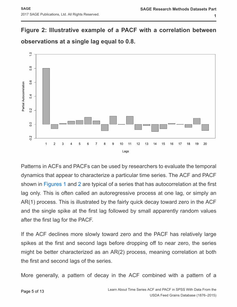
Figure 2: Illustrative example of a PACF with a correlation between

observations at a single lag equal to 0.8.

Patterns in ACFs and PACFs can be used by researchers to evaluate the temporal

dynamics that appear to characterize a particular time series. The ACF and PACF

shown in Figures 1 and 2 are typical of a series that has autocorrelation at the first

lag only. This is often called an autoregressive process at one lag, or simply an

AR(1) process. This is illustrated by the fairly quick decay toward zero in the ACF

and the single spike at the first lag followed by small apparently random values

after the first lag for the PACF.

If the ACF declines more slowly toward zero and the PACF has relatively large

spikes at the first and second lags before dropping off to near zero, the series

might be better characterized as an AR(2) process, meaning correlation at both

the first and second lags of the series.

More generally, a pattern of decay in the ACF combined with a pattern of a

SAGE



1



limited number of spikes followed by a quick drop toward zero suggests that the

series has an autoregressive process. The number of large spikes in the PACF

suggest the order of the autoregressive process – e.g. how many lags produce

independent correlations.

If a researcher observes a pattern of gradual decay in the PACF and a limited

number of spikes followed by a sharp drop to near zero in the ACF (especially

with significant negative spike for the first lag in the ACF), this suggests that

the series is better thought of as having a moving average. A moving average

effect in a time series is best thought of as an effect that impacts the values of

a series immediately and for some finite number of future periods. This contrasts

with an autoregressive process where an effect impacts future values at a steadily

declining rate through the correlation of values over time. The order of the moving

average process is suggested by how many spikes in the ACF are sufficiently

large. Thus, just like a series might have an AR(1), AR(2), or higher-order

autoregressive process, a series might also have an MA(1), MA(2), or higher-

order moving average process.

Note that the patterns that appear in ACFs and PACFs for real data are rarely

as clear as those described here. When in doubt, researchers often advocate for

the simplest structure that is consistent with the patterns revealed in the ACF and

PACF for a given time series.

Using our example of oats yield per acre, if events like droughts impacted yields

in the years in which a drought took place, but as soon as the drought ended the

impact of the drought ended, that would characterize a moving average process.

In contrast, if a new fertilizer was applied to fields in a given year and that

led to increases in yields that year, but continued to have an impact on future

yields at some steadily diminishing rate, that would characterize an autoregressive

process.

SAGE



1



A third pattern might be observed in ACFs and PACFs. If the values of the ACF

never decay all the way to zero or do so very slowly, the time series may have

a trend, which would make the series non-stationary. A stationary time series is

one where the main statistical properties of the series, such as its mean, variance,

autocorrelation, etc. are constant throughout the entire series. A trend in the data,

such as a steady increase on average over time in the values of the series,

violates the idea of a constant mean. Researchers cannot accurately diagnose

the dynamics of a non-stationary series by looking at ACFs and PACFs. The

most common treatment for non-stationarity in a time series is to calculate the

first difference of the series (also called differencing the series). You calculate the

first difference of a series by taking each observation and subtracting from it its

previous value. You then examine the ACF and the PACF of the series of first

differences to determine the remaining dynamics in the series.

Many time series might exhibit seasonal patterns or cycles in addition to the

overall AR and/or MA processes described here. For example, many economic

variables measured daily, monthly, or quarterly show seasonal cycles associated

with ebbs and flows in consumer or business behavior – holiday shopping being

a prime example. For simplicity we limit our focus to general AR and/or MA

processes.

Because ACFs and PACFs focus on computing correlations, they are most

appropriate for use when examining a continuous variable. In theory, continuous

variables are variables that can take on any numerical value within their range.

In practice, variables that take on a large number of different values within their

range are treated as continuous. Variables like age measured in years, income

measured in dollars, or unemployment measured in percentages are all good

examples.

Illustrative Example: U.S. Oats Yield per Acre, 1876–2015

SAGE



1



This example explores annual oats yield in the United States from 1876 to 2015

measured in bushels per acre. The research question is just a simple descriptive

one:

What are the temporal dynamics in annual oats yield in the U.S. over

time?

The Data

This example uses one variable from the USDA Database:

• Average oats yield in the U.S. in a given year (oatsyield), measured in

bushels per acre.

Oats yield per acre ranges from a low of 18.5 bushels per acre to a high of nearly

68 bushels per acre, with a mean of almost 40 and a standard deviation of 13.7.

There are 140 time points in the dataset, so there are 140 observations. Oats yield

per acre is a continuous variable, and it is measured once per year without gaps

for 140 years. This makes this variable appropriate for producing an ACF and a

PACF to evaluate its temporal dynamics.

Analyzing the Data

Figure 3 presents an ACF for the time series of oats yield in the United States

from 1876 to 2015 measured in bushels per acre.

Figure 3: ACF for annual oats yield per acre in the United States from

1876 to 2015, USDA Database.

SAGE



1



The ACF shows strong positive statistically significant correlations at up to 16

lags that never decay to zero. This suggests that the series is non-stationary and

should be differenced. As a result, there is no need yet to examine the PACF for

the series.

Figures 4 and 5 present the ACF and PACF of average oats yield per acre after

taking the first difference of the series.

Figure 4: ACF for first difference of oats yield per acre in the United

States from 1876 to 2015, USDA Database.

SAGE



1



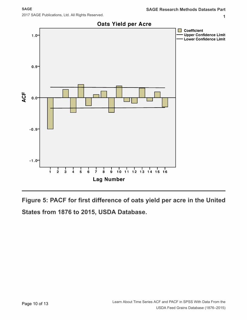
Figure 5: PACF for first difference of oats yield per acre in the United

States from 1876 to 2015, USDA Database.

SAGE



1



Figure 4 shows a moderately large negative spike at the first lag followed by

correlations that bounce around between being positive and negative and all of

which are either not statistically significant or just barely cross the threshold of

statistical significance. At the same time, Figure 5 shows what mostly looks like

a steady decay in the partial correlations toward zero. A reasonable conclusion

is that the first difference of annual oats yield is best characterized as following a

first-order moving average process.

Presenting the Results

Results for the ACF and PACF of a time series can be presented as follows:

SAGE



1



“We used a subset of data from the USDA Database reporting feed grain

production in the United States from 1876 to 2015 to evaluate the following

research question:

What are the temporal dynamics in annual oats yield in the U.S. over

time?

Figure 3 presents an autoregressive correlation function (ACF) for the time series

of annual oats yield in the United States from 1876 to 2015 measured in bushels

per acre. Figure 3 shows a series of correlations that remain large and statistically

significant out to 16 lags. The failure of the ACF to decay toward zero suggests

that the series is non-stationary and should be differenced, thereby eliminating

the need to examine the partial autoregressive correlation function (PACF) for

the series. Figures 4 and 5 present the ACF and PACF, respectively, of first

differences of annual oats yield in the U.S. The ACF in Figure 4 shows a significant

negative spike at the first lag followed by correlations that are either statistically

insignificant or nearly so. The corresponding PACF in Figure 5 shows was looks

mostly like a steady decay toward zero after the first few lags. Together, Figures

4 and 5 suggest that the series of first differences in oats yield follow a first-order

moving average process. Further analysis of the temporal dynamics of annual

oats yield should be conducted by estimating an ARIMA model.”

Review

ACFs and PACFs allow researchers to explore and identify the temporal dynamics

of an individual time series. Those dynamics may be characterized by an

autoregressive process and/or a moving average process, and may also show

evidence of non-stationarity.

You should know:

SAGE



1



• What types of variable are suitable for constructing ACFs and PACFs.

• How to produce and interpret an ACF and a PACF.

• How to report the results of an ACF and PACF for a single time series.

Your Turn

You can download this sample dataset along with a guide showing how to produce

an ACF and a PACF using statistical software. The sample dataset also includes

variables named cornyield and barleyyield, which measure the yield per acre of

corn and barley, respectively, measured in bushels over the same 140-year time

period in the United States. See if you can reproduce the results presented here,

and try producing your own ACF and PACF using one of these two new variables.

SAGE



1



Learn About Time Series ACF and PACF in SPSS With Data ...

Documents

Transcript of Learn About Time Series ACF and PACF in SPSS With Data ...