MNRAS 000, 1–15 (2013) Preprint 23 November 2015 Compiled using MNRAS LATEX style file v3.0

LEAP: the large European array for pulsars

C.G.Bassa1,2?, G.H. Janssen1,2, R.Karuppusamy3,2, M.Kramer3,2,K. J. Lee4,3,2, K. Liu3,5,2, J.McKee2, D. Perrodin6,2, M.Purver2,S. Sanidas7,2, R. Smits1,2, B.W. Stappers21ASTRON, the Netherlands Institute for Radio Astronomy, Postbus 2, 7990 AA, Dwingeloo, The Netherlands2Jodrell Bank Centre for Astrophysics, The University of Manchester, Manchester, M13 9PL, United Kingdom3Max Planck Institut fur Radioastronomie, Auf dem Hugel 69, 53121 Bonn, Germany4Kavli institute for astronomy and astrophysics, Peking University, Beijing 100871, P. R. China5Station de Radioastronomie de Nancay, Observatoire de Paris, 18330 Nancay, France6INAF - Osservatorio Astronomico di Cagliari, via della Scienza 5, 09047 Selargius (CA), Italy7Anton Pannekoek Institute for Astronomy, University of Amsterdam, Science Park 904, 1098 XH Amsterdam, The Netherlands

Accepted 2015 November 20. Received 2015 November 20; in original form 2015 July 30.

ABSTRACTThe Large European Array for Pulsars (LEAP) is an experiment that harvests the col-lective power of Europe’s largest radio telescopes in order to increase the sensitivityof high-precision pulsar timing. As part of the ongoing effort of the European PulsarTiming Array (EPTA), LEAP aims to go beyond the sensitivity threshold needed todeliver the first direct detection of gravitational waves. The five telescopes presentlyincluded in LEAP are: the Effelsberg telescope, the Lovell telescope at Jodrell Bank,the Nancay radio telescope, the Sardinia Radio Telescope and the Westerbork Synthe-sis Radio Telescope. Dual polarization, Nyquist-sampled time-series of the incomingradio waves are recorded and processed offline to form the coherent sum, resulting ina tied-array telescope with an effective aperture equivalent to a 195 -m diameter circu-lar dish. All observations are performed using a bandwidth of 128 MHz centered at afrequency of 1396 MHz. In this paper, we present the design of the LEAP experiment,the instrumentation, the storage and transfer of data, and the processing hardwareand software. In particular, we present the software pipeline that was designed toprocess the Nyquist-sampled time-series, measure the phase and time delays betweeneach individual telescope and a reference telescope and apply these delays to formthe tied-array coherent addition. The pipeline includes polarization calibration andinterference mitigation. We also present the first results from LEAP and demonstratethe resulting increase in sensitivity, which leads to an improvement in the pulse arrivaltimes.

Key words: gravitational waves — pulsars: general — methods: data analysis —techniques: interferometric

1 INTRODUCTION

Fundamental physics and our understanding of the Universeare at an important crossroad. We can now compute theevolution of the Universe back in time until a small fractionof a second after the Big Bang, and the experimental evi-dence for our standard model of particle physics has beenexemplified by the detection of the Higgs boson (Chatrchyanet al. 2012; Aad et al. 2012). At the centre of the theoret-ical understanding of both of these branches of physics are

? email: bassa@astron.nl

Einstein’s theory of general relativity (GR) and the laws ofquantum mechanics. Both theories are extremely successful,having passed observational and experimental tests with fly-ing colours (e.g. Kramer et al. 2006). Nevertheless, they seemto be incompatible, and attempts to formulate a new theoryof quantum gravity, which would unite the classical worldof gravitation with the intricacies of quantum mechanics,remain an important challenge. In this quest it is thereforehugely important to know whether GR is the right theoryof gravity after all.

Because gravity is a rather weak force, it usually re-quires massive astronomical bodies to test the predictions

c© 2013 The Authors

arX

iv:1

511.

0659

7v1

[as

tro-

ph.I

M]

20

Nov

201

5

2 Bassa et al.

of Einstein’s theory. One of these predictions involves theessential concept that space and time are combined to formspace-time that is curved in the presence of mass. As massesmove and accelerate, ripples in space-time are created thatpropagate through the Universe. These gravitational waves(GWs) are known to exist from the observed decay of theorbital period in compact systems of two orbiting stars asthe GWs carry energy away (e.g. Taylor & Weisberg 1982;Kramer et al. 2006). After inferring their existence indirectlyin this way, the next great challenge is the direct detectionof GWs.

The frequency range for which we can expect GW emis-sion from a variety of sources covers more than 20 orders ofmagnitude. Efforts to measure the displacement of masseson Earth as GWs pass through terrestrial laboratories areongoing worldwide, with the operation and upgrade of de-tectors such as (Advanced) LIGO (Abbott et al. 2009), (Ad-vanced) Virgo (Accadia et al. 2012) or GEO600 (Grote &LIGO Scientific Collaboration 2010). These detectors probeGWs at kHz-frequencies and are therefore sensitive to sig-nals from merging binary neutron stars or black hole sys-tems. At slightly lower GW frequencies, a space-based in-terferometer like the proposed eLISA observatory will besensitive to Galactic binaries and coalescing binary blackholes with masses in the range of 104 to 106 M� (Amaro-Seoane et al. 2013).

To reach a much lower GW frequency range (comple-mentary to the frequency range covered by ground-baseddetectors), we can use observations of radio pulsars. Radiopulsars are spinning neutron stars that emit beams of radioemission along their magnetic axes. The pulses of radiationdetected by radio telescopes correspond to the passing of thenarrow beam across the telescope with each rotation. Thefact that these pulses arrive with such regularity, from thebest pulsars, means that they act like cosmic clocks. In aPulsar Timing Array (PTA) experiment, we can use thesemost stable pulsars, millisecond pulsars (MSPs), as the armsof a huge Galactic gravitational wave detector, to enable adirect detection of GWs (Detweiler 1979; Hellings & Downs1983).

There are currently three major PTA experiments. InAustralia, the Parkes Pulsar Timing Array (Manchesteret al. 2013) is utilising the 64-m Parkes telescope. In NorthAmerica, NANOGrav is making use of the 100-m GreenBank Telescope (GBT) and the 305-m Arecibo telescope(Demorest et al. 2013). In Europe, the largest number oflarge radio telescopes is available: the European Pulsar Tim-ing Array (EPTA) has access to the 100-m Effelsberg tele-scope in Germany, the 76-m Lovell telescope at JodrellBank in the UK, the 94-m equivalent Westerbork SynthesisTelescope (WSRT) in the Netherlands, the 94-m equivalentNancay Radio Telescope (NRT) in France and, as the latestaddition, the 64-m Sardinia Radio Telescope (SRT) in Italy.For a recent summary of the details of the mode of operationof the EPTA, its source list and experimental achievements(e.g. the derived limits for the signal strength of a stochasticgravitational wave background or the energy scale of cosmicstring networks) and major theoretical studies, we refer toKramer & Champion (2013); Lentati et al. (2015); Desvigneset al. (submitted). All three experiments also work togetherwithin the International Pulsar Timing Array (IPTA, Hobbset al. 2010; Manchester & IPTA 2013).

Despite the apparent simplicity of a PTA experiment,the timing precision required for the detection of GWs isvery much at the limit of what is technically possible to-day. Indeed, all ongoing efforts summarised above currentlyfail to achieve the needed sensitivity (Demorest et al. 2013;Lentati et al. 2015; Shannon et al. 2013). As timing pre-cision increases essentially with telescope sensitivity (up toa point where the changing interstellar medium along theline-of-sight and the intrinsic pulse jitter become dominant,e.g. Liu et al. 2011; Cordes & Shannon 2010), an increasein telescope sensitivity is needed. In the future, radio as-tronomers expect to operate a new radio telescope known asthe Square-Kilometre-Array (SKA). The study of the low-frequency GW sky is one of the major SKA Key ScienceProjects (Janssen et al. 2014). The SKA sensitivity will beso large (ultimately up to two orders of magnitude higherthan that of the largest steerable dishes) that GW studiesmay become routine and will open up an era of GW astron-omy that will allow us to study the universe in a completelydifferent way.

In this paper, we present the first comprehensive intro-duction to the Large European Array for Pulsars (LEAP),a new experiment that uses a novel method and observ-ing mode to harvest the collective power of Europe’s largestradio telescopes in order to obtain a “leap” in the PTA sen-sitivity. The long-term aim for LEAP is to go beyond thesensitivity threshold needed to obtain the first direct detec-tion of GWs. LEAP represents the next logical, intermediatestep between the current state-of-the-art of pulsar timingand the sensitivities achievable with the SKA. The effortsand technical advances that LEAP brings (as described be-low) are essential steps towards the exploitation of the SKAand its study of the nHz-GW sky.

The LEAP experiment is introduced in §2; in §3 wedescribe the participating telescopes and the instruments;in §4 the pipelines involved in the calibration and analysisof the data are explained. The observing strategy is outlinedin §5 and initial results are presented in §6. We conclude in§7.

2 EXPERIMENTAL DESIGN

The goal of the LEAP project is to enhance the sensitiv-ity of pulsar timing observations by combining the signalsof the five largest European radio telescopes. The combina-tion of individual telescope signals can be done in two ways:coherently and incoherently. In the incoherent addition sig-nals are added after detection (squaring of the signal) henceremoving the phase information of the electromagnetic sig-nal received by the individual telescopes, so that the signal-to-noise ratio (S/N) increases with the square-root of thenumber of added telescopes1. By adapting proven techniquesfrom existing Very Long Baseline Interferometry (VLBI) ex-periments (e.g. Thompson et al. 1991), the phase delays be-tween the signals received at the individual telescopes canbe determined and corrected for, allowing for the coherentaddition of the signals (e.g. as described for LOFAR in Stap-pers et al. 2011). In this mode, the telescopes form a “tied

1 In the case of telescopes with identical apertures and receivers,

and uncorrelated noise.

MNRAS 000, 1–15 (2013)

LEAP: the large European array for pulsars 3

array” beam that is pointed to a specific sky position (herethat of a millisecond pulsar). In the standard operation modedescribed below, LEAP forms a single tied-array beam. Inthis case, the S/N of the LEAP observation is the (optimal)linear sum of the S/Ns of the individual telescopes.

Forming the coherent LEAP tied-array beam sharesmany similarities with a multi-element interferometer. Inboth cases, the individual telescopes observe the same sourceover an identical range of observing frequencies and correctthe signals of the individual telescopes for (differences in)the delays due to geometry, atmosphere, instruments andclocks. In an interferometer, the correlated signals are ul-timately used to form images with high spatial resolution,while for a tied-array, the signals from the individual tele-scopes are added coherently in phase to form the coherentsum. For short baselines of up to several kilometers, such asfor multi-element interferometers like the Australian Tele-scope Compact Array (ATCA), the Jansky Very Large Ar-ray (JVLA), the Giant Metre Radio Telescope (GMRT), theLow Frequency Array (LOFAR) and the Westerbork Syn-thesis Radio Telescope (WSRT), these corrections can beapplied in analog or digital hardware, or software, produc-ing the tied-array signal in (or near) real-time (e.g. Karup-pusamy et al. 2008; Roy et al. 2012). For longer baselines,it is usually required to store the digitized Nyquist-sampledtime-series and process the data offline. This approach isused in imaging observations for long baseline interferom-eters such as global VLBI observations or usually that ofthe European VLBI Network. Recent progress with the newSFXC software correlator would allow the formation of atied-array out of the telescopes participating in the Euro-pean VLBI Network (Kettenis & Keimpema 2014; Keim-pema et al. 2015).

The LEAP project forms a tied-array telescope specifi-cally designed to provide high S/N observations of the MSPsthat are in the EPTA (see Table 2 in Kramer & Champion2013, and also Desvignes et al. 2015). Due to the availabil-ity of sensitive L-band (1.4 GHz) receivers at all EPTA tele-scopes, LEAP observations are obtained at 1396 MHz withan overlapping bandwidth of 128 MHz. During monthly ob-serving sessions, both pulsars and suitable phase calibratorsare observed, and the data are recorded to disk. These disksare then shipped to Jodrell Bank Observatory, where thedata are correlated (in order to determine the relative phasedelays) and coherently added using software running on ahigh-performance computer cluster.

3 TELESCOPES AND INSTRUMENTS

3.1 Telescopes

We describe here in more detail the telescopes presently in-volved in LEAP:

The 100-m telescope located in Effelsberg, Germany,is a fully-steerable parabolic dish with an altitude-azimuthmount, and is operated by the Max-Planck Institut furRadioastronomie. For LEAP observations, depending onscheduling constraints, one of the two L-band (1.4 GHz)receivers (multi-beam or single-pixel) is used. Both re-ceivers provide signals corresponding to the two hands ofcircular polarization at their outputs. The receivers use

cryogenically-cooled low noise amplifiers (LNAs) based onhigh electron mobility transistors (HEMT), resulting in asystem temperature of 24 K. At L-band (1.4 GHz), the tele-scope has a gain of 1.5 K Jy−1.

The 250-foot (76.2-m) Lovell telescope at Jodrell BankObservatory has a parabolic surface with an altitude-azimuth mount. The telescope is operated by the JodrellBank Centre for Astrophysics at the University of Manch-ester. A cryogenically-cooled receiver that is placed at theprimary focus and is capable of observing a 500 MHz wideband between 1.3 and 1.8 GHz with a system temperature of25 K. This receiver has linear feeds, but uses a quarter-waveplate to produce two hands of circular polarization. The tele-scope gain for L-band (1.4 GHz) observations is 1 K Jy−1 at45◦ of elevation.

The Nancay radio telescope is a transit telescope of theKrauss design, in which the radiation is reflected via a mov-able flat mirror onto a spherical mirror, and then received ata movable focus cabin. The telescope has an equivalent di-ameter of 94 m. Depending on the declination of the source,the telescope can track sources for approximately 1 hour.The L-band receiver covers the frequency range from 1.1to 1.9 GHz with a system temperature of 35 K, and has atelescope gain of 1.4 K Jy−1 at these frequencies.

The 64-m Sardinia Radio Telescope located in SanBasilio, Sardinia, is a fully-steerable parabolic dish withan altitude-azimuth mount and a modern active surfacethat makes it one of the most technologically-advanced tele-scopes in the world. It is the newest addition to the LEAPproject. The SRT joined LEAP in July 2013 during its sci-entific validation phase. LEAP observations are done usinga cryogenically-cooled dual-band 1.4 GHz and 350 MHz con-focal receiver at the primary focus of the telescope. TheL-band receiver has a bandwidth of 500 MHz (ranging from1.3 to 1.8 GHz), a system temperature of 20 K and has linearfeeds. The corresponding telescope gain is 0.63 K Jy−1.

The Westerbork Synthesis Radio Telescope is an inter-ferometer used as a tied-array consisting of 14 equatorially-mounted, 25-m diameter, fully-steerable parabolic dishes(Baars & Hooghoudt 1974). The telescopes are equippedwith multi-frequency front-ends (MFFEs) that cover fre-quencies from 110 MHz to 9 GHz in both polarizations al-most continuously. For LEAP observations, the MFFEs aretuned to receive linearly polarized signals from eight over-lapping 20 MHz subbands between 1.3 and 1.46 GHz. Theoverlaps are necessary to match the subbands generated bythe other four LEAP telescopes. The subbands from the 25-m telescopes are separately sampled at 2-bit resolution andare then digitally combined in the tied-array adder module(TAAM), after applying the appropriate geometric delay ineach sampled subband signal. This coherently-added signalis equivalent to the signal from a 94-m diameter parabolicdish, and results in a system temperature of 27 K and a tele-scope gain of 1.2 K/Jy. Since the WSRT is currently in theprocess of transitioning to the new APERTIF observing sys-tem (Verheijen et al. 2008), for LEAP observations we haveused a varying number of 10 to 13 of the available 25-mdishes.

MNRAS 000, 1–15 (2013)

4 Bassa et al.

3.2 Instruments

To form the LEAP tied-array each observatory required aninstrument capable of recording Nyquist-sampled time-seriesover the LEAP bandwidth. These time-series are typicallyreferred to as baseband data and represent the voltages mea-sured at the telescope and sampled at the Nyquist samplingrate. For the LEAP project, these baseband recording in-struments are required to sample the two polarizations ofthe radio signal at 8-bit resolution over 128 MHz of band-width, and thus need to be capable of recording data at arate of 4 Gb s−1.

At the start of the project, VLBI baseband recordinginstruments were available at Effelsberg, Jodrell Bank andWSRT. We decided not to use those for LEAP as they usedifferent signal chains compared to the pulsar instrumentsin operation at those telescopes. Instead, we built on ourexperience gained with the PuMa II instrument at WSRT(see below), to design and build instruments for the othertelescope capable of recording baseband data. This approachallowed us to use these instruments for regular/EPTA pul-sar timing observations using DSPSR (van Straten & Bailes2011) to perform real-time coherent dedispersion and fold-ing. As such, instrumental time-offsets are minimized.

At WSRT, the TAAM generates Nyquist-sampleddata of 8 × 20 MHz subbands at a resolution of 8 bits.The PuMa II instrument (Karuppusamy et al. 2008) thenrecords the baseband data onto disks attached to separatestorage nodes. At Nancay, the BON512 instrument (Cog-nard et al. 2013) uses a ROACH FPGA board2 to sample,digitise and polyphase-filter an input bandwidth of 512 MHzat 8 bits into a flexible number of preset subbands. For stan-dard pulsar observations, the baseband data of each of thesesubbands are sent over 10Gb Ethernet to processing nodeswhere GPUs perform real-time coherent dedispersion andfolding. For the LEAP project, the disk space in one of theprocessing nodes was expanded to 55 TB to allow the base-band recording of 8× 16 MHz subbands.

At Effelsberg, Jodrell Bank and Sardinia, basebandrecording instruments were designed and built specificallyfor LEAP. These also utilise a ROACH FPGA board whereiADC analog-to-digital converters perform the digitisationand Nyquist sampling of two polarizations at 8-bit resolu-tion and for a bandwidth of up to 512 MHz. The ROACHFPGA runs firmware based on the PASP3 library blocksto perform a polyphase filterbank and generate subbands,which are subsequently packetised as UDP packets and sentover the 10Gb Ethernet network interfaces of the ROACHboard. The UDP packets are received by a cluster of com-puters where the baseband data are recorded to disk usingthe PSRDADA software4. Absolute timing is achieved bystarting the streaming of data from the ROACH at the risingedge of a one-pulse-per-second timing signal provided by theobservatory clocks. At the observatories, the ROACH iADC

2 Reconfigurable Open Architecture Computing Hardware(ROACH) FPGA board developed by the Collaboration for As-

tronomy Signal Processing and Electronics Research (CASPER)group; http://casper.berkeley.edu/3 Packetised Astronomy Signal Processor library developed by

the CASPER group.4 http://psrdada.sourceforge.net/

boards are operated at clock speeds that fully sample thebandwidth provided by the front-end, and produce at least8 subbands with a bandwidth of 16 MHz. The analog signalchain at the observatories are set up so that the center fre-quencies of these subbands are 1340, 1356, 1372, 1388, 1404,1420, 1436 and 1452 MHz, respectively.

The baseband data generated during LEAP observa-tions from WSRT, Nancay, Effelsberg and Sardinia are sentto Jodrell Bank, where the correlation and further process-ing is done on a dedicated computer cluster, as described inSects. 3.3 and 4.

3.3 Storage and processing hardware

To facilitate the storage and transfer of data from the re-mote observatories to Jodrell Bank, storage computers withremovable disks were installed at Effelsberg, WSRT and Sar-dinia. During LEAP observations, the raw baseband data ofeach telescope are recorded onto the disks of the instrument.At the end of the observing run, the data are transferred tothe local storage machine and the removable disks are thenshipped to Jodrell Bank, where they are placed into similarstorage computers for offline processing. After processing hasfinished, the removable disks are shipped back to the remoteobservatories for re-use.

The baseband data obtained at Jodrell Bank are imme-diately transferred over the internal network to one of thestorage computers, while the presence of a fast data-link be-tween Nancay and Jodrell Bank allows the data obtained atNancay to be transferred directly over the internet to one ofthe storage computers at Jodrell Bank.

At Jodrell Bank, a high performance computer clusteris used to correlate and coherently add the baseband datafrom the individual telescopes. The cluster consists of 40nodes, each with two Quad core Intel Xeon processors, 8 GBof RAM and 2 TB of storage.

4 DATA PROCESSING PIPELINE ANDCALIBRATION

A software correlator and beamformer were developedspecifically for the LEAP project to process the single-telescope baseband data and form the coherent addition ofthese data. The correlator and beamformer are part of a dataprocessing pipeline that automates most of the processing.

4.1 Data processing pipeline

A flowchart of the LEAP processing pipeline is shown inFig. 1. The processing starts once the baseband data of each16 MHz subband from all LEAP telescopes from one of theobserving sessions are online at the central storage machineat Jodrell Bank Observatory.

During the first processing stage, the data from eachtelescope are correlated to find the exact time and phaseoffsets between the telescopes. This is achieved by first ap-plying an initial time offset corresponding to the geomet-ric delay, the clock delay and the hardware delay by sim-ply shifting one of the time-series by an integer number ofsamples with respect to the other. The remaining time de-lay is a fraction of a time sample (see § 4.2). The baseband

MNRAS 000, 1–15 (2013)

LEAP: the large European array for pulsars 5

Figure 1. A flowchart of the LEAP data processing pipeline. Each observatory stores the baseband data from single-telescope LEAP

observations on disk. The data are then transferred to the central storage machine at Jodrell Bank Observatory. There, polarizationcalibration and RFI mitigation filters are applied to the single-telescope data, which are then correlated, resulting into a fringe-solution

for each of LEAP’s baselines (ten telescope pairs in total). At this stage, we apply the fringe-solution to each telescope’s baseband data

(again after polarization calibration and RFI mitigation), correlate the time-series again, and check the resulting ‘visibilities’ to verifythat the fringe-solution is indeed correct. The baseband data (to which the fringe-solution is applied) are then added together in phase,

forming the LEAP tied-array. The added baseband data are processed as normal timing data. The data is then dedispersed and folded(using DSPSR) and template matching is performed to produce the final pulse times-of-arrival (TOAs).

data are then Fourier-transformed (channelized) to the fre-quency domain to form complex frequency channels. This isperformed in time segments of typically 100 samples, lead-ing to 100 frequency channels for each time-segment. Thepolyphase filters implemented in the digital instruments atEffelsberg, Jodrell Bank, Nancay and Sardinia provide com-plex valued time-series, requiring the complex-to-complexFourier transform to channelize the data. In the case ofWSRT, real-valued time-series are created and the real-to-complex Fourier transform is used to generate the channel-ized complex time-series. When converted to the frequencydomain, the polarization is converted from linear to circularand the polarization calibration is applied (§ 4.3). At thisstage the RFI mitigation methods are also applied (§ 4.5).The remaining fractional delay is corrected for by rotatingthe complex values of each frequency channel in phase. Thecorresponding complex time-series for each baseline pair andfrequency channel are then correlated to form ’visibilities’.As such, the correlator is of the FX design, where the Fouriertransform (F) is followed by the correlation (X), similar toother software correlators like DiFX (Deller et al. 2007) andSFXC Keimpema et al. (2015).

The visibilities are averaged in time, allowing the resid-ual time and phase offsets between each pair of telescopesto be extracted by applying the global fringe fitting methodfrom Schwab & Cotton (1983). An initial Fourier transformmethod is used to find a fringe solution to within one sam-ple. This solution is then applied to a least-squares algorithmthat makes use of phase closure and involves minimizing thedifference between model phases and measured phases bysolving for the phase offset of each telescope (fringe phase),the time slope (fringe delay) and the phase drift (fringe rate).The fits are performed independently on both left-hand-

circular and right-hand-circular polarizations. The resultingfringe rates are averaged over both polarizations.

During the second processing stage, the exact time andphase offsets with respect to a reference telescope are appliedto the baseband data from each telescope. An amplitudescaling is also applied to these data to ensure maximumsensitivity (see Sect. 4.4).

4.2 Phase calibration and pulsar gating

Creating the LEAP tied-array beam requires the basebanddata from each telescope to be corrected for an appropri-ate time delay and phase shift before they can be addedcoherently. The time and phase delays between the time-series from individual telescopes consists of four components.First, the largest delays are due to differences in geome-try that result in different path lengths that the signal hasto travel. Second, there are differences between each ob-servatory’s local clocks. The third component consists ofinstrument-specific delays due to cables and electronic com-ponents. Finally, the atmosphere (both ionosphere and tro-posphere) introduces a delay as a time-varying phase-shiftof the radio-wavefront, which depends on the time-varyingconditions of the local atmosphere as well as the wavelengthsof the radio waves5.

The geometric delays can be largely corrected for byusing the known terrestrial positions of the telescopes, tele-scope pointing models and celestial position of the source(calibrator or pulsar). The long baselines in LEAP meanthat our tied-array beam is very small and it is therefore

5 The chosen observing frequency for LEAP of 1.4 GHz lies in a

regime where both tropospheric and ionosperic effects are small.

MNRAS 000, 1–15 (2013)

6 Bassa et al.

essential to have an accurate position for the right epoch. Itis therefore vital to include any known proper motion termswhen calculating the true position for the observing epoch.For LEAP, these delays are calculated using the CALC6

program (Ryan & Vandenberg 1980). For our pipeline, wemake use of a C-based wrapper for CALC, which is part ofthe DiFX software correlator (Deller et al. 2007). Applyingthe geometric delays and clock delays requires a referencelocation and a reference time standard. We have chosen toreference the time series of the individual telescopes to theEffelsberg telescope. This choice was made primarily becausethe Effelsberg telescope is the one with the largest aperture.Because the time and phase delays are determined on base-lines that include Effelsberg, the corrections are relative, notabsolute. As a consequence, the corrected and subsequentlyadded baseband time-series can be treated for further anal-ysis as if they were observed by Effelsberg in terms of thegeometric delays and clock offsets normally used in pulsartiming.

The delays from the signal-path and the atmosphereare measured by correlating the baseband data of the tele-scopes using the purpose-built LEAP software. An initialfringe-solution of the residual time and phase differences be-tween each pair of telescopes is found by correlating a cal-ibrator source. However, the calibrator source is typicallyoffset by about 5◦ from the pulsar and separated in timeby several minutes. Because of this, the conditions of theionosphere/troposphere for the calibrator observation willbe different than for the pulsar observation, leading to a dif-ferent fringe-solution. Thus, when the fringe-solution fromthe calibrator is applied to the pulsar data, it does not yieldperfect coherence (see Fig. 2). In addition, the conditions ofthe ionosphere/troposphere can change unpredictably on atimescale of minutes, as shown in Fig. 3. This means thatthe observation would need to be interrupted to observe thecalibrator at least once every 15 minutes (or even every 5minutes in case the ionospheric conditions are very poor).As part of the processing pipeline, we therefore developeda procedure to allow the phase-calibration to be performedon the pulsar signal itself. This method of calibrating on thetarget is called self-calibration and widely used in interfer-ometry.

To do this, we implemented a pulse binning techniqueto optimize the sensitivity. The visibilities within each in-dividual pulse are integrated into bins with a size equal toa fraction of the pulse period. This is done for each fre-quency channel. The bins from each individual pulse are thenadded (folded) to the corresponding bins from all previouspulses, using TEMPO to predict the exact pulse period. Atime-shift is applied to each individual channel to correct forthe dispersion delay. This results in average visibilities foreach pulsar phase bin, for each frequency channel and foreach baseline. Finally, the bins containing the on-pulse sig-nal are selected (this is the process of gating) and averagedtogether. This yields visibilities for each baseline where onlythe on-pulse signal of the pulsar contributes, and increasesthe signal-to-noise ratio roughly by a factor equal to thereciprocal of the square-root of the duty cycle. This proce-

6 CALC is part of the Mark-5 VLBI Analysis Software

Calc/Solve

dure allows the fringes to be tracked over time on the pulsarsignal itself as the conditions of the ionosphere/tropospherechange, removing the need to switch between pulsar andcalibrator during the observation. Phase calibrating on thetarget source uses the positional information of the pulsar,and hence this approach can not be used for astrometry.

Once the total time and phase delays for each tele-scope with respect to the reference telescope have been de-termined, they are applied to the raw data in two stages.First, the baseband data from each telescope are aligned tothe nearest integer sample (62.5 ns for a complex sampledsubband of 16 MHz). The remaining fractional time delay(a fraction of a sample) plus the measured delay in phase,is corrected for by phase rotating the complex values of thechannelized time-series. After these corrections, the channel-ized time-series from each telescope correspond in both timeand phase with the time-series from the reference telescope.These channelized time-series can thus be added togethercoherently.

Finding a fringe-solution after correlating the time-series from the telescopes can be impeded by a lack ofpulsar signal, rapidly changing conditions of the iono-sphere/troposhere, extreme cases of RFI, or – in the caseof Nancay – by an irregular clock-drift7. In those instanceswhere no fringe-solution can be obtained, the time-series areadded incoherently. The time series are then corrected forthe known time-delays by applying the geometric delay cor-rection, the clock correction, the instrumental delays and thefringe-solution from the calibrator, which aligns the signalsto within a few tens of ns. Once the signals are time-aligned,they are added without consideration of the relative phaseof the electromagnetic signal received by the individual tele-scopes. This is achieved by simply adding the power of thebaseband data. For incoherent addition, the signal-to-noiseratio increases with the square-root of the number of addedtelescopes8.

4.3 Polarization calibration

To maximize the coherency of the tied-array beam, it iscrucial to perform accurate polarization calibration that re-moves the effects introduced by the telescope, receiver andinstrument. This is particularly important for LEAP, as eachof the individual telescopes is of a different design, uses dif-ferent receivers and feeds, and we are observing pulsars forwhich parts of the average pulse profiles are up to 100%-polarized. In Fig. 4 we compare uncalibrated pulse profileswith profiles after calibration using the method describedbelow.

Here we briefly describe the LEAP polarization cali-bration scheme, the details of which will be presented ina forthcoming paper. In LEAP, polarization calibration is

7 The rubidium clock that is providing the timing signals for theLEAP pulsar backend has typically two correction values per day

with respect to the time standard at Paris-Meudon Observatory.

The clock drift can be as large as 10 ns within one hour, and cansometimes deviate from linear drift.8 In the case of telescopes with identical apertures and receivers,

and uncorrelated noise.

MNRAS 000, 1–15 (2013)

LEAP: the large European array for pulsars 7

-3

-2

-1

0

1

2

3

1340 1360 1380 1400 1420 1440 1460

Fri

nge-

phas

e (r

ad)

Frequency (MHz)

-3

-2

-1

0

1

2

3

1340 1360 1380 1400 1420 1440 1460

Fri

nge-

phas

e (r

ad)

Frequency (MHz)

Figure 2. Fringe solution from a calibrator versus the fringe

solution from the pulsar itself. These two panels show thevisibility phase between the baseband time-series from Effels-

berg and WSRT from the first 5 minutes of an observation of

PSR J1022+1001, taken on February 24, 2015. The x-axis showsthe observing frequency from 1332 to 1460 MHz. The y-axis shows

the visibility phase between the two time-series for each frequency

channel (in units of radians). The top graph shows the visibilityphase from the calibrator (taken 6 min before the pulsar observa-

tion), applied to the pulsar observation. The bottom graph shows

the fringe from the pulsar observation itself. A visibility phase ofzero over the whole bandwidth means that the two signals are

perfectly in phase and will thus add fully coherent. A residual

time-offset between the two time-series will show up as a slope.The phase-calibrator is offset from the pulsar by 3◦ on the sky.

performed for each telescope independently, before corre-lating and finding the fringes. Performing polarization cal-ibration has two major benefits. First, it helps to improvethe S/N of fringe solutions, i.e. to determine accurate phaseoffsets between telescopes. Second, performing polarizationcalibration after coherent addition is complicated, since ex-tra phases have been introduced in the addition process. Infact, the expected S/N of an un-calibrated fringe will be 22%lower than the calibrated one, assuming random differentialphase between the two hands of polarization and a 100%polarized signal. It is thus hard to evaluate the polarizationperformance of each telescope, and check the data integrityindividually.

For single telescope systems, the distortion of polar-

-10

-8

-6

-4

-2

0

0 500 1000 1500 2000 2500 3000

frin

gep

has

e (r

ad)

time (s)

EB-JB LHCEB-JB RHC

EB-WB LHCEB-WB RHC

Figure 3. The evolution of the fringe-phase over time. The fourlines show the drift in the fringe-phase in radians of a calibra-

tor observation for the two baselines Effelsberg-Jodrell Bank and

Effelsberg-WSRT for both polarizations: left-hand circular (LHC)and right-hand circular (RHC). It demonstrates that both the ab-

solute value of the fringe-phase as well as the time-derivative of

the fringe-phase (called fringe-drift) can change significantly on atimescale of minutes.

ization can be described by seven system parameters9.For a quasi-monochromatic wave, there are two majorparametrization schemes. In Britton’s scheme (Britton2000), there are: the total gain, spinor transformation axes(four parameters) and the transformation rotation angles(two parameters). In Hamaker’s scheme (Hamaker et al.1996), there are: the total gain, the gain-phase imbalance(two parameters), leakage amplitude and phase (four pa-rameters). The two descriptions are equivalent. We adoptthe Hamaker scheme in the LEAP pipeline, however we donot assume that the polarization distortions are small, sincewe are working with an inhomogeneous array.

The aforementioned system parameters can be mea-sured by comparing the observed full-Stokes pulsar pulseprofile to the standard profile templates. The standard χ2

fitting minimizing the differences between the template andthe modeled profile is used to fit for the system parame-ters of each frequency channel. In this way, the pulsar it-self is also used as the polarization calibrator in our obser-vations. PSR J1022+1001 and/or PSR B1933+16, for whichthe pulse profiles show significant amounts of both linear andcircular polarization components, are normally used for po-larization calibration. Our approach is similar to the matrixtemplate matching method by van Straten (2006), exceptthat we calibrate baseband data directly.

There are three major steps in our algorithm. First,the observed pulse profile is aligned with a template pro-file (using the algorithm of Taylor 1992). Next, non-linearχ2-fitting is used to derive the system parameters. Thesesystem parameters are then applied to the observed profilein order to estimate the post-calibrated profile. These stepsare repeated until the solution converges, that is when the

9 The 2× 2 complex Jones matrix has 8 real parameters that are

required to specify it. However, the total phase shift is determined

by fringe fitting, so only 7 parameters are required. The numberof parameters can be reduced to 6 if one is not interested in the

gain calibration.

MNRAS 000, 1–15 (2013)

8 Bassa et al.

Figure 4. Pulsar profiles of PSR J1022+1001 as observed with the individual telescopes before and after polarization calibration. The

solid, dashed, and dotted curves, are for total intensity, linear polarization, and circular polarization respectively. The top row are theprofile without calibration, and the bottom row are the calibrated ones. The EB, JB, NCY, and WB abbreviations indicate the Effelsberg,

Jodrell, Nancay, and Westerbork telescopes. Here the y-axis, flux, takes an arbitrary unit, and x-axis is pulse phase. The calibrated profiles

clearly show much better consistency.

fractional changes of the system parameters are smaller than10−7. Our results show that the above iteration convergesmost of the time, and that we can measure both the sys-tem parameters and the phase offsets between the templateand measured pulse profile at the same time. This proce-dure is similar to using a noise diode as a calibrator. How-ever, because of the change of polarization angle across thepulse profile, we are no longer limited to the case of single-axial calibration, and are able to fix the whole set of systemparameters, including leakage terms. Indeed, we need to in-clude such terms to fully calibrate the Nancay data. Figure 5shows the improvement in visibility phases after calibratingthe polarization.

4.4 Amplitude calibration

To ensure maximum S/N of the added data, we have to applyan appropriate weight to the baseband data from each of thetelescopes, where we have to consider that the final addeddata are written as 8-bit samples. To achieve this, we selecta reference telescope and measure the noise-levels from thebaseband data from each telescope and set the weights suchthat all samples are scaled to the noise-levels of the referencetelescope. We then take the S/N from the average intensityprofiles from the individual telescopes and scale the weightswith an additional factor given by:

Wtel =

√S/Ntel

S/Nref

,

where S/Ntel is the S/N of the telescope and S/Nref is theS/N of the reference telescope. This ratio of the S/N includesthe telescopes’ system temperature relative to that of thereference telescope. The voltage samples from each of thetelescopes are then multiplied by the corresponding weightbefore the addition, which maximizes the S/N of the addeddata. At this stage, the samples are floating point numbers.After the addition, a final scaling is applied such that thestandard deviation of the samples becomes one third of thedynamic range of 8-bit data. This ensures minimal clippingand optimal use of the dynamic range when the data is con-verted to 8-bit and written to disk.

4.5 Interference mitigation

In case of significant radio frequency interference (RFI), wehave implemented two methods to clean the data. The RFImitigation step is optional and performed right after thecalibration. These RFI mitigation methods are applied tothe channelized data from the individual telescopes beforecoherent addition.

The first form of RFI-mitigation consists of selectingand masking frequency channels that contain narrow-bandRFI. These channels are selected via a simple algorithm thatlooks for channels with an integrated power exceeding eithera given threshold or deviating significantly from its neigh-bors. These channels are then masked by replacing the con-tent with Gaussian noise with mean and rms determinedfrom neighboring time samples.

A second technique can be applied to data contain-

MNRAS 000, 1–15 (2013)

LEAP: the large European array for pulsars 9

1364 1366 1368 1370 1372 1374 1376 1378 1380

f (MHz)

−100

−50

0

50

100

150

200

250

300

∆Φ

(◦)

un-calibrated, rms = 35◦

calibrated rms = 20◦

−100 −50 0 50 100

∆Φ (◦)

0

2

4

6

8

10

12

14

16

18

Cou

nts

un-calibratedcalibrated

Figure 5. This figure illustrates the effects of the polarization

calibration for a 10-second integration of a 16 MHz subband of

the Effelsberg-Nancay baseline. The top panel shows the visibilityphase ∆Φ as a function of frequency with and without applying

of the polarization calibration. A histogram of these phase delays

with and without applying the polarization calibration is shownin the bottom panel. For this example, the average S/N of the

visibilities shows an 18% increase after polarization calibration,and the corresponding phase error is reduced by 40%, i.e. the rms

level of the visibility phase reduced is from 35◦ to 20◦.

ing time-varying RFI, or broadband RFI. This techniqueimplements the method of spectral kurtosis (Nita & Gary2010a,b) to remove RFI from some observations. It providesunbiased RFI removal with a resolution of 6.25 ms in timeand 0.16 MHz in frequency. In each frequency channel andat each telescope, the distribution of a time-series of 1000samples of total power is assessed for similarity to that ex-pected from Gaussian-distributed amplitudes. This is doneusing an estimator that measures the variance divided bythe square of the mean for these power samples. When thepower is derived from Gaussian amplitudes of zero mean,the estimator has a probability density function (PDF) thatis independent of the variance of those amplitudes. It cantherefore be used to distinguish RFI on the premise thatnon-Gaussian amplitudes are caused by RFI. The PDF isused to determine three-sigma limits for the estimator, anda block of 2000 amplitude samples (1000 in each polariza-tion channel) is masked if it gives an estimator value outsidethese limits. This excludes 0.27% of RFI-free data, whileexcluding most RFI-contaminated data. The amplitudes ofRFI-contaminated samples are replaced by artificial Gaus-

0 0.50.40.30.20.1 10.90.80.70.6

0 0.50.40.30.20.1 10.90.80.70.6

Pulse phase

02

40

24

Ap

pro

xim

ate

Ela

pse

d T

ime

(m

in)

Figure 6. Pulsar phase-vs-time plot of coherently-added LEAP

data of PSR J1022+1001, without (top) and with the spectralkurtosis RFI mitigation method (bottom). The observation was

taken on July 27, 2013 with Effelsberg, Jodrell Bank, Nancay, andWSRT. There was significant broadband RFI from the Nancay

observation, which dramatically changed the baseline of the

coherently-added integration profile, as shown in the top panel.After applying the filter to Nancay data only, the resulting LEAP

data are significantly improved.

sian noise with the same variance as nearby samples, in orderto maintain a constant noise level in the correlated ampli-tudes regardless of the number of telescopes contributingto each sample. As before, the masked data is replaced byGaussian noise.

We cannot generally define the percentage of RFI-contaminated data that is excluded, because we do notknow, a priori, the PDF of the estimator derived from thesedata. Some RFI-contaminated data may not be excluded iftheir PDF closely mimics that of Gaussian amplitudes. How-ever, our practical application has shown it to be effective inautomatically removing the vast majority of the dominantRFI that would otherwise spoil our correlations (see Fig. 6).It is also possible that a very strong pulsar signal could bemisinterpreted as RFI by the spectral kurtosis method butthat does not happen when using the time and frequencyresolutions employed by LEAP.

5 OBSERVING STRATEGY

LEAP observations are crucial in that they complementthe regular, more frequent multi-frequency observations ofthe EPTA by adding time-of-arrival measurements with thehighest possible precision. Observing sessions for LEAP arescheduled with an approximately monthly cadence, each ses-sion lasting a minimum of 24 hours. During each observingsession, a set of millisecond pulsars and phase calibratorsare observed simultaneously with each of the five radio tele-scopes. Since the first observations of June 2010, the ob-serving time per session, number of pulsars per session, andnumber of participating telescopes per session have steadilyincreased.

Initial testing to aid in software development used eight

MNRAS 000, 1–15 (2013)

10 Bassa et al.

Table 1. Pulsars and calibrators observed for the LEAP project. Notes: a) PSR J1518+4904 cannot be observed simultaneously with

all five telescopes, therefore the Jodrell Bank, Effelsberg, and Sardinia telescopes observe PSR J1738+0333 instead. b) PSR B1933+16 is

used for polarization calibration as explained in Sect. 4.3 and is not included in the PTA list. Telescope codes: E: Effelsberg; J: JodrellBank; N: Nancay; S: Sardinia; W: WSRT.

Pulsar Calibrator length (min) telescopes Pulsar Calibrator length (min) telescopes

J0029+0554 3 EJNSW J1719+0817 3 EJNSWJ0030+0451 40 EJNSW J1713+0747 50 EJNSW

J0037+0808 3 EJNSW J1719+0817 3 EJNSW

J0606−0024 3 EJNSW J1740+0311 3 EJSJ0613−0200 60 EJNSW J1738+0333a 60 EJS

J0616−0306 3 EJNSW J1740+0311 3 EJS

J0619+0736 3 EJSW J1740−0811 3 EJNSWJ0621+1002 45 EJSW J1744−1134 45 EJNSW

J0619+0736 3 EJSW J1752−1011 3 EJNSW

J0743+1714 3 EJSW J1821−0502 3 EJNSWJ0751+1807 40 EJSW J1832−0836 35 EJNSW

J0743+1714 3 EJSW J1832−1035 3 EJNSW

J0927−2034 3 EJNSW J1847+0810 3 EJNSWJ0931−1902 40 EJNSW B1855+09 50 EJNSW

J0932−2016 3 EJNSW J1847+0810 3 EJNSW

J0957+5522 3 EJSW J1926−1005 3 EJSWJ1012+5307 45 EJSW J1918−0642 20 EJSW

J0957+5522 3 EJSW J1926−1005 3 EJSW

J1015+1227 3 EJNSW B1933+16b 5 EJNSWJ1022+1001 45 EJNSW B1937+21 45 EJNSW

J1025+1253 3 EJNSW J1946+2300 3 EJNSW

J1028−0844 3 EJSW J2006−1222 3 EJNSWJ1024−0719 45 EJSW J2010−1323 55 EJNSW

J1028−0844 3 EJSW J2011−1546 3 EJNSW

J1506+4933 3 NW J2130−0927 3 EJNSWJ1518+4904a 60 NW J2145−0750 45 EJNSW

J1535+4957 3 NW J2155−1139 3 EJNSW

J1554−2704 3 EJNSW J2232+1143 3 EJNSWJ1600−3053 60 EJNSW J2234+0944 35 EJNSW

J1607−3331 3 JNSW J2241+0953 3 EJNSW

J1641+2257 3 EJSW J2303+1431 3 EJNSWJ1640+2224 50 EJSW J2317+1439 40 EJNSW

J1641+2257 3 EJSW J2327+1524 3 EJNSW

J1638−1415 3 EJNSWJ1643−1224 35 EJNSW

J1638−1415 3 EJNSW

of the single 25-m WSRT dishes, obtaining 20 MHz of band-width for a set of 6 millisecond pulsars. These data were usedto test software beamforming and allow a comparison withthe output of the WSRT hardware beamformer. The firstlong-baseline observations were obtained in June 2011 usingWSRT and Effelsberg. These observations initially used fivesubbands of 20 MHz, but switched to the 8× 16 MHz setupstarting in February 2012, when the Lovell telescope at Jo-drell Bank was included in the LEAP array. The Nancaytelescope first joined in May 2012, initially with 4× 16 MHzsubbands, and since December 2012 with the full 128 MHzbandwidth. Test observations with the SRT were obtained inJuly 2013 for one 16 MHz subband. Tests with one subbandwere then performed monthly until January 2014. Finally,thanks to the successful installation of an 8-node computercluster, the telescope joined full-length and full-bandwidthLEAP sessions in March 2014.

Through a memorandum of understanding between the

participating telescopes and institutes, observing time at Jo-drell Bank, Nancay and SRT is guaranteed, while for Effels-berg and WSRT, the observing runs are proposed throughthe peer-review process at these telescopes. The long-termscheduling at Effelsberg and WSRT thus guides the schedul-ing of the LEAP observing sessions, which are matched bythe Lovell, Nancay and Sardinia telescopes.

Besides the principal requirement that the observedsources be simultaneously visible from all sites, the observ-ing schedule takes the individual telescope constraints intoaccount for each LEAP session. The primary observing con-straint is set by the transit design of Nancay, where sourcesare visible for 60 to 90 minutes around culmination, depend-ing on the declination of the source. The altitude-azimuthmounts of the Effelsberg, Lovell and Sardinia telescopes usu-ally do not allow observations at very small local zenith-angles (i.e. LEAP observations avoid zenith angles of lessthan 10◦), and have slew limits at certain azimuths related

MNRAS 000, 1–15 (2013)

LEAP: the large European array for pulsars 11

to cable wrapping. The equatorial design of WSRT limits ob-servations to hour angles from −6 to +6 h around transit foreach source. Furthermore, WSRT requires a 3-min initializa-tion time between observations to configure the tied-array.This initialization time overlaps with the slewing time for alltelescopes, as well as with a minimum observing length re-quirement of 6 min for all observations done with the LovellTelescope. The slewing rates, minimum observing time andinitialization time mostly impact the calibrator observationsbefore and after each pulsar observation, which are generallyonly three minutes long. To obtain the most efficient overallobserving schedule and a maximum overlap between all tele-scopes for each observation, LEAP requires all observationsto end at the same time.

Besides the telescope constraints, the visibility of MSPssuitable for pulsar timing array experiments also provides astringent constraint on the schedule. To first order, the mostsuitable pulsars are clustered towards the inner Galacticplane, with very few pulsars at right ascensions between 01h

and 05h. Furthermore, to maximize the number of sourcesthat are visible at Nancay, it is beneficial to include sourcesseparated equally in right ascension. To maximize the num-ber of suitable MSPs observable by LEAP, we moved awayfrom continuous 24-hour observing sessions. Since the springof 2013, we observe in two sessions, spanning right ascensionranges from 06h00m to 01h30m and 15h30m to 21h00m. Thetwo parts of a full LEAP run are usually separated by onlya day. Table 1 lists the pulsars and phase calibrators ob-served by LEAP. The current selection of pulsars is basedon an optimization of using the best pulsars observed bythe EPTA (Desvignes et al. submitted), while following theobserving restrictions explained above. This results in somehigh-quality pulsars in crowded areas of the sky being ob-served by less than 5 telescopes, or not being included at all;this also means that some pulsars that are not necessarilythe best PTA sources are included in the list.

6 RESULTS

Processing of LEAP data is presently ongoing. During thesecond half of 2014 the processing pipeline reached a level ofmaturity that allowed us to transition to a scheme wherebythe data of one epoch was processed and analyzed beforethe data of the next epoch was obtained. Here, we presentresults obtained from data from these epochs, as well as datafrom a few specific epochs prior to the second half of 2014,which have been processed during the development phase ofthe pipeline.

6.1 Coherence

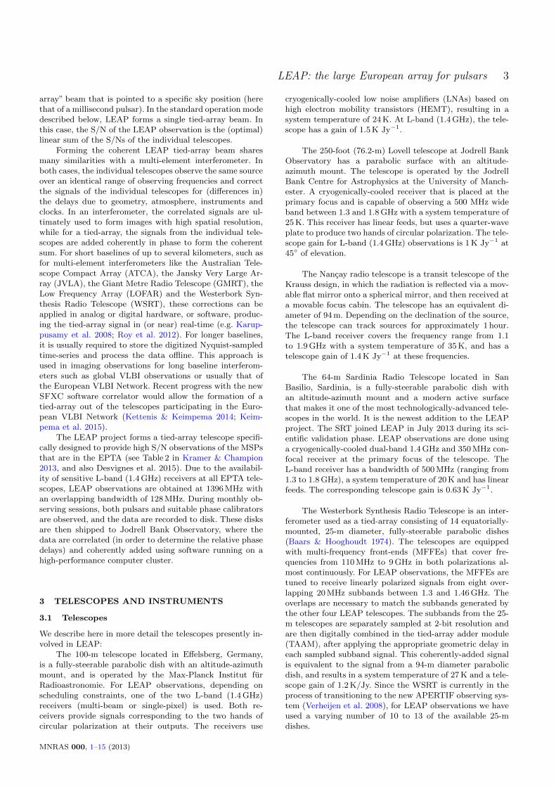
The correlation and addition of single-telescope basebanddata using the LEAP data reduction pipeline producesLEAP data with the expected coherence. An example of suchcoherence is shown in Fig. 7, where we present the pulse pro-file of PSR J1022+1001 from LEAP data compared to theprofiles from single-telescope data (all scaled to the off-pulserms). In Fig. 8 we present the S/Ns of all the LEAP profilesfor PSR J1022+1001, compared to those of the individualdishes, for the months in which the pulsar signal was strongenough to perform coherent addition. Full coherent addition

Figure 7. Pulsar profiles of PSR J1022+1001 from individual

telescopes and their coherent addition, normalized based on theiroff-pulse rms. The raw data were obtained at MJD 56500, with

an integration time of 30 minutes. The peak signal-to-noise ratios

of Effelsberg, Jodrell Bank, Nancay, WSRT and LEAP, are 97,51, 42, 30, 220, respectively, which corresponds to a near perfect

coherency.

is achieved when the time series of the individual telescopesare perfectly in phase. The LEAP S/N should then be sim-ilar to the sum of the S/Ns of the individual telescopes.Fig. 7 and 8 show that the S/N for LEAP is close to thesum of the S/Ns of the individual telescopes, demonstratingthat LEAP is achieving full coherent addition when thereis sufficient signal. Deviations from the maximum S/N canbe caused by an inaccurate fringe-solution (possibly due toresidual RFI or due to a non-linear phase-drift), or due toimproper polarization or amplitude calibration (see Sect. 4.3and 4.4).

With LEAP observing there are three possible datacombinations. The most sensitive of these is clearly whenwe combine all the dishes involved coherently over the fullLEAP bandwidth. In the few cases where coherent additionis not possible the incoherent sum of the available dishes,over the LEAP bandwidth, gives us the best sensitivity. Thisassumes that a sufficient number of dishes (i.e. more than2) is involved in the sum. Otherwise, the incoherent combi-nation of the TOAs, as opposed to the raw data, from thewide bandwidth observations from the individual telescopesis used. This is because the sensitivity of the incoherent sumscales as the square-root of the number of dishes while thesensitivity of the combination of the TOAs determined fromthe wide-band data scales as the square-root of the ratio ofthe bandwidth available to the dishes over that available toLEAP. In all cases we end up with a better result for theoverall sensitivity compared to what would be possible witha single telescope observation from one of the LEAP dishes.

Based on the LEAP observations that have been fullyprocessed at the time of submission of this paper, 51% ofthe sources were processed coherently with more than 80%coherency, 8% were processed coherently with 60 to 80% co-herency, and the remaining 41% were processed incoherently.The reasons for the poor coherency achieved for some of thepulsars are a combination of poor S/N due to scintillation,imperfect polarization calibration, large or non-linear fringedrifts due to ionospheric conditions or the Nancay clock, andRFI across the LEAP band.

While these coherence numbers are lower than hoped,we have already improved our polarization calibration rou-tines and our RFI mitigation procedures as described else-

MNRAS 000, 1–15 (2013)

12 Bassa et al.

0

500

1000

1500

2000

55967

56192

56500

56945

57009

57077

S/N

MJD

LEAP

EB

JB

NRT

SRT

WSRT

Figure 8. S/Ns from LEAP vs. S/Ns from the individual tele-

scopes for PSR J1022+1001 for the observations where coherentaddition could be performed. The earliest observation shown is

from February 2012, the last observation shown is from February

2015. The graph shows that the LEAP data provides the expectedimprovement in S/N, meaning that the sum of the S/Ns of the

individual telescopes is roughly identical to the S/N of LEAP.

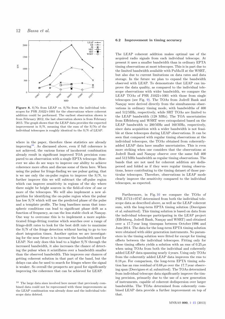
where in the paper, therefore these statistics are alreadyimproving10. As discussed above, even if full coherence isnot achieved, the various forms of incoherent combinationalready result in significant improved TOA precision com-pared to an observation with a single EPTA telescope. How-ever we also do see ways to improve our ability to achievecoherence more often and discuss some of them here. Whenusing the pulsar for fringe-finding we use pulsar gating, thatis we use only the on-pulse region to improve the S/N, tofurther improve this we will subtract the off-pulse regionwhich can improve sensitivity in regions of the sky wherethere might be bright sources in the field-of-view of one ormore of the telescopes. We will also implement a new al-gorithm for identifying the on-pulse region when the pulsarhas low S/N which will use the predicted phase of the pulseand a template profile. The long baselines mean that iono-spheric conditions can lead to significant phase drift as afunction of frequency, as can the less stable clock at Nancay.One way to overcome this is to implement a more sophis-ticated fringe-fitting routine which searches over a range offringe-drift rates to look for the best drift rate to maximisethe S/N of the fringe detection without having to go to tooshort integration times. Another option we are investigat-ing for the near future is to increase the bandwidth used forLEAP. Not only does this lead to a higher S/N through theincreased bandwidth, it also increases the chance of detect-ing the pulsar when it scintillates over a bandwidth smallerthan the observed bandwidth. This improves our chances ofgetting coherent solution in that part of the band, but thedelays can also be used to search for fringes where the signalis weaker. So overall the prospects are good for significantlyimproving the coherence that can be achieved for LEAP.

10 The large data sizes involved here meant that previously com-bined data could not be reprocessed with these improvements asthe LEAP combination was already done and the individual tele-

scope data deleted.

6.2 Improvement in timing accuracy

The LEAP coherent addition makes optimal use of theacquired radio signals from each individual telescope. Atpresent it uses a smaller bandwidth than in ordinary EPTAtiming observations at most telescopes. This is in part due tothe limited bandwidth available with PuMa II at the WSRT,but also due to current limitations on data rates and datastorage. In the future we plan to expand the bandwidthobserved with LEAP. To demonstrate that LEAP can im-prove the data quality, as compared to the individual tele-scope observations with wider bandwidth, we compare theLEAP TOAs of PSR J1022+1001 with those from singletelescopes (see Fig. 9). The TOAs from Jodrell Bank andNancay were derived directly from the simultaneous obser-vations in ordinary timing mode, with bandwidths of 400and 512 MHz, respectively, while SRT TOAs are limited tothe LEAP bandwidth (128 MHz). The TOA uncertaintiesfrom Effelsberg and WSRT were extrapolated based on theLEAP bandwidth to 200 MHz and 160 MHz, respectively,since data acquisition with a wider bandwidth is not feasi-ble at these telescopes during LEAP observations. It can beseen that compared with regular timing observations at theindividual telescopes, the TOAs obtained from coherently-added LEAP data have smaller uncertainties. This is evenmore striking when one considers that the observations atJodrell Bank and Nancay observe over the same full 400and 512 MHz bandwidth as regular timing observations. Thebands that are not used for coherent addition are dedis-persed and folded as if they were regular timing observa-tions, hence contributing to the timing dataset of those par-ticular telescopes. Therefore, observations in LEAP modeclearly improve the sensitivity compared to the individualtelescopes, as expected.

Furthermore, in Fig. 10 we compare the TOAs ofPSR J1713+0747 determined from both the individual tele-scope data as described above, as well as the LEAP coherentsum, with the long-term EPTA timing solution (Desvigneset al. submitted). This timing solution is based on data fromthe individual telescope participating in the LEAP project(Effelsberg, Jodrell Bank, Nancay and WSRT) and obtainedover a 17.7 year long timespan between October 1996 andJune 2014. The data for the long-term EPTA timing solutionwere obtained with older generation instruments. No param-eters in the timing solution were fitted for except for timingoffsets between the individual telescopes. Fitting only forthese timing offsets yields a solution with an rms of 0.25µswhen using TOAs from both the individual and coherentlyadded LEAP data spanning nearly 4 years. Using only TOAsfrom the coherently added LEAP data improves the rms to0.18µs. For comparison, the long-term EPTA timing solu-tion has an rms residual of 0.68µs over the 17.7 year observ-ing span (Desvignes et al. submitted). The TOAs determinedfrom individual telescope data significantly improve the tim-ing precision, primarily due to the use of a new generationof instruments, capable of coherent dedispersion over largerbandwidths. The TOAs determined from coherently com-bined LEAP data provide a further improvement on top ofthat.

MNRAS 000, 1–15 (2013)

LEAP: the large European array for pulsars 13

0.1

1

57077

57009

56945

56500

56192

55967

σT

OA (

µs)

TOA number

LEAPEBJB

NRTSRT

WSRT

Figure 9. TOA uncertainties from LEAP for PSR J1022+1001

compared with those obtained from single-telescope data, which

were acquired simultaneously but with broader bandwidth. Thefull ordinary bandwidths of Jodrell Bank and Nancay are 400

and 512 MHz, respectively. The TOA uncertainties from Effels-berg and WSRT were extrapolated from 128 MHz to 200 and

160 MHz, respectively (these are the bandwidths used in the or-

dinary on-site EPTA timing campaigns). The available EPTAtiming bandwidth at SRT is currently the same as LEAP.

Figure 10. Timing residuals of PSR J1713+0747 obtained fromsingle telescope data (colored points), as well as the coherently

added LEAP data (black points). These residuals are computedby comparing the TOAs against the long-term EPTA timing so-lution of PSR J1713+0747 (Desvignes et al. submitted). No pa-

rameters, other than timing offsets between the telescopes, werefitted for. Over this five year timespan the data from the individ-

ual telescopes participating in LEAP, as well as the coherently

added LEAP data presently available, allow the timing solutionto be constrained to an rms of 0.25µs. The solution using onlyTOAs determined from the coherently added LEAP data has an

rms of 0.18µs. For the Jodrell Bank and Nancay telescopes theTOAs from the data obtained over the full instrument bandwidth

are shown.

6.3 Phase jitter and single pulse studies

LEAP delivers a sensitivity that is rivaled only by Arecibo,the largest single-dish radio telescope on Earth. The dataare therefore ideal for studies of the phase jitter of inte-grated profiles and single pulses of MSPs, which are not oftenfeasible with single-telescope data due to low S/N. Fig. 11

-1.5

-1

-0.5

0

0.5

1

1.5

-0.006 -0.004 -0.002 0 0.002 0.004

Re

sid

ua

l (µ

s)

MJD-56193.7

Figure 11. Timing residuals of PSR J1713+0747 over a period

of 15 min, for each 10-s integration. The observations were per-

formed on MJD 56193, included Effelsberg, Nancay, and WSRT,and the generation of the LEAP data achieved a coherency of

95%. The rms residual is 522 ns and the corresponding reducedχ2 is 9.47.

shows an example of such an analysis for PSR J1713+0747.The observations were carried out with Effelsberg, Nancay,and WSRT on MJD 56193. The plot shows timing resid-uals for 10-s integrations for a 15-min observing time. TheTOA errors corresponding to measurement uncertainties dueto radiometer noise were estimated by the classic templatematching method (Taylor 1992). To calculate the residu-als, we used the ephemeris from the EPTA timing release(Desvignes et al. submitted) without fitting for any param-eters. We see that the error bars clearly underestimated thescatter of the residuals, which is an indicator of phase jitter(e.g. Liu et al. 2011). The rms residual is 522 ns with a re-duced χ2 of 9.47. Following the method in Liu et al. (2012),this leads to an estimated jitter noise of 494 ns for a 10-s in-tegration time. This is consistent with previously publishedresults (Shannon & Cordes 2012; Dolch et al. 2014). Fromthe coherently-added LEAP data, we also managed to obtainsingle pulses of the pulsar with fully-calibrated polarizationat a time resolution of 2.2µs, an example of which can befound in Fig. 12. The single pulses have sharp features andsignificant linear polarizations. Further investigation of thesingle pulses from PSR J1713+0747 will be presented in aseparate paper.

6.4 Pulsar searching

The increased sensitivity of the LEAP tied array allowssearches for weak pulsars with known positions. Thoughthe LEAP tied array beam of the full LEAP array is small,beamforming can be used to tile out the incoherent beam.

As a proof of concept, we have performed a blind searchon 5 min of coherently-added LEAP data of the double neu-tron star PSR J1518+4904, with the aim of detecting pul-sations from the second neutron star. The baseband datawere acquired at MJD 56193 with Effelsberg and the WSRT,and were later combined with nearly full coherency. The re-sulting Nyquist-sampled timeseries of each 16-MHz subbandwere then used to form a filterbank file with 1-MHz channels.Next we combined the filterbank files from each individual

MNRAS 000, 1–15 (2013)

14 Bassa et al.

Figure 12. Polarization profile of a single pulse from

PSR J1713+0747, obtained from the observation used in Fig. 11.

subband to yield the full observing bandwidth and used thePRESTO software package to search for pulsations.

In total, 33 candidates were detected with the same DMas PSR J1518+4904, all of which were harmonics of the pul-sar or attributed to RFI. No pulsations with a non-harmonicperiod were found from an initial investigation down to aflux limit of 0.31 mJy. As PSR J1518+4904 is part of themonthly LEAP observing sessions, we will be able to use allcoherently-combined data on this system for the most sen-sitive search to date for radio emission from its neutron starcompanion.

7 CONCLUSIONS AND PROSPECTS

In this paper we present an overview of the LEAP project,which coherently combines data from up to five 100-m classradio telescopes in Europe, forming a tied-array telescope.We observe a subset of the EPTA MSPs with a sensitiv-ity that cannot be achieved by the individual participatingtelescopes. The LEAP project emerges as a natural result ofthe many years of collaboration between the EPTA groups.Instead of merely sharing their TOAs for GW detection pur-poses, the EPTA telescopes in the LEAP project are com-bined using VLBI techniques to form a fully-steerable 195-mequivalent dish, forming one of the most sensitive pulsar ob-servation instruments to date.

We describe the LEAP setup and operation, startingfrom the data acquisition setup at the participating tele-scopes, the transfer of data to the centralized LEAP com-puting infrastructure at Jodrell Bank, to the final processingof the monthly LEAP observing runs. We have also pre-sented the main characteristics of the pipeline that was de-veloped for the processing the data. We describe the chal-lenges of achieving high timing precision, in great part dueto the many differences in the telescopes and their pulsarobserving systems. These differences were managed eitherfully in software (incorporated into the LEAP pipeline), orwith hardware upgrades when these were inevitable. The de-velopment of our own end-to-end pipeline (individual tele-scope data, polarization calibration, RFI mitigation, corre-lator and tied-array adder) not only provided us with theflexibility to overcome all of these obstacles, but also al-

lowed us to take the most out of each telescope. The effortsplaced into making LEAP a reality have however been re-warded by the quality of the results. As we have shown, thecoherency of the added individual telescope data can reach100%. In addition, the TOA uncertainty of the LEAP datais less than that of the individual telescopes, even thoughthe LEAP bandwidth is a few times smaller.

Although the main aim of LEAP is to provide high pre-cision pulsar timing data towards a direct detection of GWs,its high sensitivity and flexibility as an observing system en-able it to go beyond this scope and pursue broader pulsar-related science. Pulse phase jitter and single pulse studies,which are demanding in terms of sensitivity, are ideal forLEAP. This was best demonstrated with the single pulsedetections of PSR J1713+0747 during one of the standardLEAP observations. We have also demonstrated that LEAPis capable of performing targeted pulsar searches in a casestudy using PSR J1518+4904. Even though its current op-eration mode does not allow it to be used as a generic pulsarsearching instrument, its high sensitivity makes it a perfecttool for investigating known binaries and looking for pulsa-tions from pulsar companions in order to identify double-pulsar systems. Moreover, LEAP has recently been used toobserve the Galactic center magnetar PSR J1745−2900 atfrequencies higher than used in the typical LEAP runs, inorder to determine the scattering properties of the ISM to-wards the Galactic centre. This study used VLBI imagingtechniques and helped define the best search strategies forpulsars close to Sgr A∗ (Wucknitz 2015).

The addition of LEAP data to the current PTA datasets will significantly improve PTA data quality. We are cur-rently finalizing the LEAP timing data set of the data ob-tained to date, and will use these data to perform a search forGWs and place upper limits on the GW amplitude. We canalready extrapolate the results of our currently processeddata to the full time span of 3.2 years, by counting thenumber of telescopes that joined each observing session. As-suming 90% coherency and using the red noise parametersof each pulsar measured from the much longer EPTA dataset, we can calculate the statistics of the expected timingnoise and measurement accuracy, then derive upper limitson the amplitude of the GW background using a Cramer-Rao bound. For a spectral index of −2/3 (i.e. a stochasticGW background dominated by supermassive binary blackholes), the LEAP upper limit on the dimensionless strainamplitude Ac is Ac(1yr−1) ≤ 1.2×10−14, using extrapolateddata of four LEAP pulsars, PSR J0613−0200, J1022+1001,J1600−3053, and J1713+0747. With only 3.2 years of data,such an upper limit is a factor 2 to 5 higher compared to thepublished results that used 10-year long data sets and morepulsars (van Haasteren et al. 2011; Demorest et al. 2013;Shannon et al. 2013; Lentati et al. 2015).

Dedicated funding for the LEAP project officially endedin September 2014. However, the unique character and thesuccess of LEAP have justified its continuation at all par-ticipating telescopes, which have provided the necessarymonthly observation time. While this paper provides anoverview of the LEAP project, several papers are presentlyin preparation that provide details of the instrumentation,pipeline and the calibration, as well as present results fromthe LEAP project.

MNRAS 000, 1–15 (2013)

LEAP: the large European array for pulsars 15

ACKNOWLEDGEMENTS

The European Pulsar Timing Array (EPTA) is a collab-oration of European institutes to work towards the directdetection of low-frequency gravitational waves and to im-plement the Large European Array for Pulsars (LEAP).The authors acknowledge the support of the colleagues inthe EPTA. In particular, we would like to thank the fol-lowing colleagues for their great help with our instrumen-tation, observations and administrative issues (in alphabet-ical order): I. Cognard, G. Desvignes, B. Dickson, A. Hol-loway, C. Jordan, P. Lespagnol, A. G. Lyne, P. Stanway,G. Theureau, and WeiWei Zhu. In Sardinia we would liketo thank the SRT Astronomical Validation Team, and inparticular: M. Burgay, S. Casu, R. Concu, A. Corongiu, E.Egron, N. Iacolina, A. Melis, A. Pellizzoni and A. Trois. Weare grateful to A. Deller, M. Kettenis and Z. Paragi for shar-ing their knowledge of VLBI. The work reported in this pa-per has been funded by the ERC Advanced Grant “LEAP”,Grant Agreement Number 227947 (PI M. Kramer). KJL ac-knowledge support from National Basic Research Programof China, 973 Program, 2015CB857101 and NSFC 11373011.The 100-m Effelsberg Radio Telescope is operated by theMax-Planck-Institut fur Radioastronomie at Effelsberg. TheWesterbork Synthesis Radio Telescope is operated by theNetherlands Institute for Radio Astronomy (ASTRON) withsupport from The Netherlands Foundation for Scientific Re-search (NWO). The Nancay Radio Observatory is operatedby the Paris Observatory, associated with the French CentreNational de la Recherche Scientifique. Pulsar research at theJodrell Bank Centre for Astrophysics and the observationsusing the Lovell Telescope are supported by a consolidatedgrant from the STFC in the UK. The Sardinia Radio Tele-scope is operated by the Istituto Nazionale di Astrofisica(INAF) and is currently undergoing its astronomical valida-tion phase.

REFERENCES

Aad G., Abajyan T., Abbott B., Abdallah J., Khalek S. A., 2012,

Physics Letters B, 716, 1

Abbott B. P., et al., 2009, Reports on Progress in Physics, 72,

076901

Accadia T., et al., 2012, Journal of Instrumentation, 7, 3012

Amaro-Seoane P., et al., 2013, GW Notes, Vol. 6, p. 4-110, 6, 4

Baars J. W. M., Hooghoudt B. G., 1974, A&A, 31, 323

Britton M. C., 2000, ApJ, 532, 1240

Chatrchyan S., Khachatryan V., Sirunyan A., Tumasyan A.,

Adam W., Aguilo E., 2012, Physics Letters B, 716, 30

Cognard I., Theureau G., Guillemot L., Liu K., Lassus A., Desvi-gnes G., 2013, in Cambresy L., Martins F., Nuss E., PalaciosA., eds, SF2A-2013: Proceedings of the Annual meeting of theFrench Society of Astronomy and Astrophysics. pp 327–330

Cordes J. M., Shannon R. M., 2010, preprint, (arXiv:1010.3785)

Deller A. T., Tingay S. J., Bailes M., West C., 2007, PASP, 119,

318

Demorest P. B., et al., 2013, ApJ, 762, 94

Detweiler S., 1979, ApJ, 234, 1100

Dolch T., et al., 2014, ApJ, 794, 21

Grote H., LIGO Scientific Collaboration 2010, Classical and

Quantum Gravity, 27, 084003

Hamaker J. P., Bregman J. D., Sault R. J., 1996, A&AS, 117, 137

Hellings R. W., Downs G. S., 1983, ApJ, 265, L39

Hobbs G., et al., 2010, Classical and Quantum Gravity, 27, 084013

Janssen G. H., et al., 2014, in Advancing Astrophysics with the

Square Kilometre Array.

Karuppusamy R., Stappers B., van Straten W., 2008, PASP, 120,191

Keimpema A., et al., 2015, Experimental Astronomy, 39, 259

Kettenis M., Keimpema A., 2014, in Proceedings of the 12th Eu-ropean VLBI Network Symposium and Users Meeting (EVN

2014). 7-10 October 2014. Cagliari, Italy.. p. 88Kramer M., Champion D. J., 2013, Classical and Quantum Grav-

ity, 30, 224009

Kramer M., et al., 2006, Science, 314, 97Lentati L., et al., 2015, MNRAS, 453, 2576

Liu K., Verbiest J. P. W., Kramer M., Stappers B. W., van Straten

W., Cordes J. M., 2011, MNRAS, 417, 2916Liu K., Keane E. F., Lee K. J., Kramer M., Cordes J. M., Purver

M. B., 2012, MNRAS, 420, 361

Manchester R. N., IPTA 2013, Classical and Quantum Gravity,30, 224010

Manchester R. N., et al., 2013, Publ. Astron. Soc. Australia, 30,

17Nita G. M., Gary D. E., 2010a, PASP, 122, 595

Nita G. M., Gary D. E., 2010b, MNRAS, 406, L60Roy J., Bhattacharyya B., Gupta Y., 2012, MNRAS, 427, L90

Ryan J. W., Vandenberg N. R., 1980, in Bulletin of the American

Astronomical Society. p. 457Schwab F. R., Cotton W. D., 1983, AJ, 88, 688

Shannon R. M., Cordes J. M., 2012, ApJ, 761, 64

Shannon R. M., et al., 2013, Science, 342, 334Stappers B. W., et al., 2011, A&A, 530, A80

Taylor J. H., 1992, Royal Society of London Philosophical Trans-

actions Series A, 341, 117Taylor J. H., Weisberg J. M., 1982, ApJ, 253, 908

Thompson A. R., Moran J. M., Swenson G. W., 1991, Interfer-

ometry and synthesis in radio astronomyVerheijen M. A. W., Oosterloo T. A., van Cappellen W. A.,

Bakker L., Ivashina M. V., van der Hulst J. M., 2008,in Minchin R., Momjian E., eds, American Institute of

Physics Conference Series Vol. 1035, The Evolution of Galax-

ies Through the Neutral Hydrogen Window. pp 265–271(arXiv:0806.0234), doi:10.1063/1.2973599

Wucknitz O., 2015, ArXiv:1501.0451,

van Haasteren R., et al., 2011, MNRAS, 414, 3117van Straten W., 2006, ApJ, 642, 1004

van Straten W., Bailes M., 2011, Publ. Astron. Soc. Australia,

28, 1

This paper has been typeset from a TEX/LATEX file prepared by

the author.

MNRAS 000, 1–15 (2013)