Application Note 71

Synchronization ±

Jitter ± Wander:

Basic principles and

test equipment

An ANT-20 application

Wandel & GoltermannCommunications Test Solutions

Leading the Way with Innovative

Jitter & Wander Test Solutions

O.172

2

Contents

1 Introduction 3

2 Definition and sources of jitter 3

2.1 What are jitter and wander? 3

2.2 Sources of jitter and wander 3

2.3 Disruptions caused by jitter 4

2.4 Disruptions caused by wander 4

2.5 How do you measure jitter

and wander? 4

3 Jitter applications 5

3.1 Measuring output jitter 5

3.2 Measuring the maximum tolerable

jitter (MTJ) 8

3.3 Measuring the jitter transfer function

(JTF) 10

3.4 Measuring mapping jitter 11

3.5 Measuring combined jitter 13

4 Synchronization 15

4.1 Synchronization network architecture 15

4.2 How does clock regeneration work? 16

4.3 Clock derivation in network elements 17

4.4 Usage of timing markers 17

4.5 Clock compensation using

pointer actions 19

4.6 Test applications 20

5 Wander applications 21

5.1 Wander measurement 21

5.2 Offline wander analysis 24

6 Jitter and wander test equipment 28

Appendix: Jitter and wander standards 30

Abbreviations

ADM Add Drop MultiplexerANSI American National Standards InstituteAU Administrative UnitBITS Building Integrated Timing SourceDS-x Digital Signal, Level xDWDM Dense Wavelength Division MultiplexE1 2.048 kbit/s linkETSI European Telecommunication

Standardization InstituteFAS Frame Alignment SignalGPS Global Positioning SystemGSM Global System for Mobile

CommunicationsITU International Telecommunication UnionJTF Jitter Transfer FunctionLOF Loss of FrameLOS Loss of SignalMTIE Maximum Time Interval ErrorMTJ Maximum Tolerable JitterNDF New Data FlagNE Network ElementO.171 ITU-T Recommendation for jitter and

wander measurement on electricalinterfaces of PDH systems

O.172 ITU-T Recommendation for jitterand wander measurement onelectrical & optical interfaces ofSDH/SONETsystems

OC Optical CarrierPDH Plesiochronous Digital HierarchyPLL Phase Locked LoopPOH Path Overheadppm Parts per Million (10-6)PRC Primary Reference ClockPRS Primary Reference SourceRDI Remote Defect IndicationREI Remote Error IndicationRMS Root Mean SquareRx ReceiverS1 Synchronization Status Byte

(Timing Marker)SDH Synchronous Digital HierarchySEC SDH Equipment ClockSOH Section OverheadSONET Synchronous Optical NetworkSSU Synchronization Supply UnitSTM Synchronous Transport ModuleSTS Synchronous Transport SignalTIE Time Interval ErrorTSE Test Sequence ErrorTU Tributary UnitTx TransmitterUI Unit Interval

Publishing details

Authors:Jochen Hirschinger, Wolfgang Miller

Published by:Wandel & Goltermann GmbH & Co.Elektronische MeûtechnikMuÈ hleweg 5D-728000 Eningen u. A.Germany

Subject to change without noticeOrder no. TP/EN/A071/0799/AEPrinted in Germany

The ANT-20 Advanced NetworkTester is the world standardwhen it comes to transmissiontest solutions. The ANT-20is a modular platform offeringPDH, SDH, SONET andATM capabilities, and theinstrument can be flexiblyconfigured to handle extremelydiverse customer requirements.The jitter test & measurementfacilities are one importantcomponent:. Jitter/wander measurements

at all major bit rates (electricaland optical): E1, E3, E4,STM-1/4/16 or DS1, DS2,DS3, STS-1/3/12,OC-1/3/12/48

. Complete compliance withITU-T Rec. O.172 for com-parable, insightful and precisemeasurement results

. Using the Zoom function, thegraphical results presentationformat lets you detect errorsin the details even with long-term measurements (also use-ful for acceptance reports)

. Automation with the ªCATSTest Sequencerº softwareincreases the efficiency ofcommonly occurring tests andlong-term measurements

. PC-based design, Windowsgraphical user interface (GUI),touchscreen: Practically anyquantity of results and setupscan be stored to hard disk.Floppy disk drive for ex-changing data. Offline analysisof stored results is possibleon any PC. PCMCIA slotssimplify installation ofmodems and/or LAN cards.

1 Introduction

2 Definition and sources of jitter

2.1 What are jitter and wander?

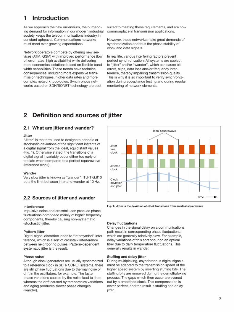
JitterªJitterº is the term used to designate periodic orstochastic deviations of the significant instants ofa digital signal from the ideal, equidistant values(Fig. 1). Otherwise stated, the transitions of adigital signal invariably occur either too early ortoo late when compared to a perfect squarewave(reference clock).

WanderVery slow jitter is known as ªwanderº. ITU-T G.810puts the limit between jitter and wander at 10 Hz.

2.2 Sources of jitter and wander

InterferenceImpulsive noise and crosstalk can produce phasefluctuations composed mainly of higher frequencycomponents, thereby causing non-systematic(stochastic) jitter.

Pattern jitterDigital signal distortion leads to ªintersymbolº inter-ference, which is a sort of crosstalk interferencebetween neighboring pulses. Pattern-dependentsystematic jitter is the result.

Phase noiseAlthough clock generators are usually synchronizedto a reference clock in SDH/ SONETsystems, thereare still phase fluctuations due to thermal noise ordrift in the oscillators, for example. The fasterphase variations caused by the noise lead to jitter,whereas the drift caused by temperature variationsand aging produces slower phase changes(wander).

Delay fluctuationsChanges in the signal delay on a communicationspath result in corresponding phase fluctuations,which are generally relatively slow. For example,delay variations of this sort occur on an opticalfiber due to daily temperature fluctuations. Thisgenerally results in wander.

Stuffing and delay jitterDuring multiplexing, asynchronous digital signalsmust be adapted to the transmission speed of thehigher speed system by inserting stuffing bits. Thestuffing bits are removed during the demultiplexingprocess. The gaps which then occur are evenedout by a smoothed clock. This compensation isnever perfect, and the result is stuffing and delayjitter.

3

As we approach the new millennium, the burgeon-ing demand for information in our modern industrialsociety keeps the telecommunications industry inconstant upheaval. Communications networksmust meet ever-growing expectations.

Network operators compete by offering new ser-vices (ATM, GSM) with improved performance (lowbit error rates, high availability) while deliveringmore economical solutions based on flexible band-width capabilities. These trends have technicalconsequences, including more expensive trans-mission techniques, higher data rates and morecomplex network topologies. Synchronous net-works based on SDH/SONET technology are best

suited to meeting these requirements, and are nowcommonplace in transmission applications.

However, these networks make great demands ofsynchronization and thus the phase stability ofclock and data signals.

In real life, various interfering factors preventperfect synchronization. All systems are subjectto ªjitterº and/or ªwanderº, which can cause biterrors, slips, data loss and/or frequency inter-ference, thereby impairing transmission quality.This is why it is so important to verify synchroniz-ation during acceptance testing and during regularmonitoring of network elements.

Ideal squarewave

Time

Jitter-freeclock

Jitteredclock

Clockdeviationand jitter

Fig. 1: Jitter is the deviation of clock transitions from an ideal squarewave

Mapping jitter

Plesiochronous and asynchronous signals aremapped into synchronous containers using stuffingtechniques. At the next terminating multiplexer, theplesiochronous tributaries are then unpacked. Dueto the stuffing that occurred, there are gaps in therecovered signal, which are compensated usingPLL circuitry. There is still some leftover phasemodulation, which is known as mapping or stuffingjitter (see section 3.4)

Pointer jitter

Clock differences between two networks orbetween SDH network elements are compensatedby pointer movements. These pointer jumpscorrespond to 8 or 24 bits, depending on themultiplex hierarchy. When the tributary signal isunpacked at the end point, the phase variationsare still present but are smoothed out usingPLL circuitry. The residual phase modulation isknown as pointer jitter. Besides pointer jitter, theunpacked signal also exhibits mapping jitter, sothe sum total of both, known as ªcombinedº jitter(see section 3.5), is always measured.

2.3 Disruptions caused by jitter

It is the job of clock recovery circuitry used innetwork elements to correctly sample the digitalsignal, i.e. as close as possible to the center of thebit, using the recovered bit clock. If the digitalsignal and the clock both have identical jitter, thenthe position of the sampling instant does notchange despite significant jitter error. Sampling stilloccurs properly, and no bit errors arise. Strictlyspeaking, however, this is the case only with low-frequency jitter for which the clock recoverycircuitry can keep up with digital signal phasevariations with no problems. At higher jitterfrequencies, however, the clock recovery circuitrycannot keep up with the fast phase variations ofthe digital signal. Phase shifts result, and for values40.5 clock periods (UI = Unit Interval), the result isincorrect sampling of the bit element and thus biterrors.

Due to additional digital signal distortion, thedecision range is much smaller in real life. At verylarge jitter amplitudes, bit errors become socommon that a loss of frame (LOF) will occur.

2.4 Disruptions caused by wander

Unlike jitter, the phase variations due to wanderdo not lead to bit errors since the recovered clockcan easily follow these slow changes in phase.However, wander amplitudes can accumulate toproduce very large values over longer time inter-vals. Digital signals arriving at network and ex-change nodes from different directions can havevery high wander amplitudes relative to one an-other. Since digital signals are processed internallywith a common clock, buffers are required tocompensate for the wander.

At SDH/SONET nodes, these buffers can berelatively small since adaptation is possible usingpointer actions. However, pointer actions can leadto a high jitter amplitude in the transported payloadsignal at the tributary output.

At exchange nodes, however, if the buffer over-flows the only way to compensate involves anintentional frame slip. Parts of the transmittedsignal are lost, producing error bursts. However,these error bursts do not trigger alarms due to aloss of frame (LOF) or errors in the frame alignmentsignal (FAS).

2.5 How do you measure jitterand wander?

Jitter effects

To measure jitter effects, the incoming signal isregenerated to produce a virtually jitter-free signal,which is used for comparison purposes. No ex-ternal reference clock source is required for jittermeasurement. The maximum measurable jitterfrequency is a function of the bit rate and ranges at2.488 Gbit/s (STM-16/OC-48) up to 20 MHz. Theunit of jitter amplitude is the unit interval (UI), where1 UI corresponds to an error of the width of one bit.Test times on the order of minutes are necessary toaccurately measure jitter.

Wander effects

Wander test equipment requires an external, ex-tremely precise reference clock source. The mostpractical unit of wander amplitude is the absolutemagnitude in ns (10±9 seconds), and not the UI unitpreferred for jitter measurements. The extremelylow frequency components (mHz range) requirerather long test times ranging up to 106 s.

4

The differences between jitter and wander are alsoreflected in the various test applications, eventhough in both cases we are dealing with phasefluctuations that must be measured and evaluated(Table 1). See section 6 for a basic descriptionof the operation of a jitter/wander test set and asummary of the standards.

3 Jitter applications

3.1 Measuring output jitter

A certain amount of jitter will appear at the outputof a network element even if an entirely jitter-freedigital signal or clock is applied to its input. TheNE itself produces this ªintrinsicº jitter. Reasonsare as follows:

. Thermal noise in clock oscillators

. Spurious emissions by crystals in clockoscillators

. Influences from other system modules on theclock supply (crosstalk)

. Pattern-dependent delay in scramblers andencoders

. Insufficient edge steepness in digital signals

Prior to installing network elements, it is importantto measure the output jitter to assure that themaximum values are not exceeded (see Appendix,Table 1). This helps avoid interoperability problemswith other network elements as well as jitter-relatedtransmission impairments (Fig. 2).

There are separate standards for the output jitter ofnetwork interfaces (see Appendix, Table 2), andcompliance is important to assure that the jittertolerance is not violated at any network interfaces.This type of test is particularly important whenconnecting links/paths between two different net-work operators. It should therefore be part of anystandard acceptance procedure.

The values should be checked within specified jitterbandwidths. There are usually two jitter values:One for high-frequency jitter and one for broad-band jitter (see also section 6: ªJitter weightingº)

Test principleThe signal under test is connected to the ANT-20'sreceiver (Fig. 2). The test set's transmitter feeds anacceptable signal to the input of the device undertest (DUT) in order to prevent an alarm from beingtriggered. The test duration is variable, i.e. it is notgoverned by any standards. Experience shows thata duration of 5 minutes works fine. The importantparameter here is the maximum peak-to-peak jitter(UIpp) during the test interval.

5

Jitter Wander

Frequency range ofphase variations

410 Hz 0±10 Hz

Primary disruption Causes bit errors Synchronizationproblems

Reference clock sourcefor measurement

Not required Absolutely necessary

Unit for amplitude UI (Unit Interval) ns

Test times Minutes Long-term measure-ment (hours, days)

Table 1: Comparison between jitter and wander, including consequencesfor test equipment

Tx

Rx

Jitter measurement

Networkelement

Tx

RxNetwork

Jitter measurement

Fig. 2: Measuring the output jitter of network elements and interfaces

3.1.1 Displaying the test results

With its graphical and numerical display facilities,the ANT-20 can show the test results in a tableor as a measurement curve, with the followingpossibilities:

± Current values± Maximum values within a specific test interval± Results vs. time

With the many display options, you can systemati-cally analyze and identify reasons for increasedjitter and correlate the jitter with transmissionerrors (Figs. 3 and 4). See the box on p. 7 for anexplanation of jitter parameters.

Displaying instantaneous valuesYou can measure the peak-to-peak or root meansquare (RMS) value of the jitter. Phase hits can alsobe counted (see terminology on p. 7). Fig. 3 showshow results are presented for a peak-to-peak jittermeasurement. The test set determines the positiveand negative values for a phase variation (leadingand lagging edges). Phase hits are recorded at thesame time. The results are updated continuously(ªCurrent Valuesº). The ªMax. Valuesº occurringduring a specific test interval are also noted anddisplayed at the end of the measurement.

ªJitter vs. timeº display modeYou can record the peak-to-peak or root meansquare (RMS) value of the jitter vs. time. Thispresentation format is particularly useful for long-term in-service monitoring and for troubleshooting.The ANT-20 offers a number of possibilities forin-service analysis. For example, anomalies anddefects can be recorded with a time-stamp duringa long-term jitter measurement. This helps tocorrelate increased jitter and transmission errors.The graphics make it easier to identify extremevalues. For example, if increased bit errors occuron an operational link, this helps you to systemati-cally identify the problem.

6

Fig. 3: Numerical results window showing jitter peak valuesand phase hits

Fig. 4: The jitter vs. time measurement. Negative and positivepeak values can be recorded, or peak-to-peak values.

Example:Jitter accumulation in regenerators

Regenerators generally do not use the sameprecision clock sources as other network elements.Accordingly, jitter is not so highly suppressed.This means that in a chain of generators, jitter canaccumulate to yield values which can exceedtolerable limits in some cases.

The RMS value is useful for qualifying the intrinsicjitter of regenerators. Assuming the jitter is non-systematic, the ªpower lawº can be invoked,meaning you can simply add the individual jitterpower components for each regenerator in thechain.

The RMS value of the jitter at the output of a chainof N regenerators can be computed based on thefollowing formula:

J = HJREG12 + JREG2

2 + ... +JREGN2

ÐÐÐÐÐÐÐÐÐÐÐÐÐÐÐÐÐÐÐÐÐÐÐÐÐÐÐÐÐÐÐÐÐÐÐÐÐÐÐÐÐÐÐÐÐÐÐÐÐÐÐÐÐÐÐ

For N identical regenerators, the formula can besimplified:

J = HN ´ JREG

ÐÐб

Now we can compute the maximum tolerable jittervalue for a regenerator to avoid exceeding themaximum jitter (Jmax ) at the end of a chain ofN regenerators:

JREG = Jmax/HN (N = Number of regenerators)ÐÐÐÐ

The maximum tolerable output jitter for networkelements and networks is given in the Appendix(Tables 1 and 2).

7

Fig. 5: Definition of jitter amplitude UIpp

Jitter (UIpp) Jitter amplitude(peak-to-peak value)

Test time

Definition of jitter parameters

Unit Interval (UI)Measure of jitter amplitude. 1 UI correspondsto an amplitude of one bit clock period. Theunit interval UI is independent of bit rate andsignal coding since it is referred to the lengthof a clock period.

Peak-to-peak valueThe distance between the highest and lowestjitter value is known as the jitter amplitude.It is measured as a peak-to-peak value UIpp

(Fig. 5).

Phase hitsA measurement of peak-to-peak jitter saysnothing about how often the tolerable jitteramplitudes are exceeded. Phase hits are jitterpeaks that exceed an (adjustable) amplitude.Based on a count of phase hits, you can betterevaluate jitter behavior. The ªJitter vs. timeºpresentation also shows how phase hits aredistributed over time (see Fig. 4).

RMS jitterThe root mean square (RMS) value of the jittersignal provides an indication of the jitter noisepower. Peak values that cause bit errors arenot recorded by an RMS measurement.Only the quadratic mean is obtained, but theintegration time is not standardized. Somestandards (e.g. ITU-T G.958, ANSI T1.105.03)use RMS measurement to characterizeregenerators (see example below).

STM-NOC-M Regenerator

1

Regenerator2

Regenerator3

Jitter power

Jitter power

Reg 1

Reg 2

Reg 1

Jitter power

Reg 3

Reg 2

Reg 1

Fig. 6: The jitter accumulation for a chain of regenerators is computed by addingthe RMS values (ªpower lawº)

3.2 Measuring the maximum tolerable jitter (MTJ)

The optical and electrical inputs of transmissionand tributary interfaces must be able to toleratespecific jitter amplitudes (MTJ, maximum tolerablejitter) without loss of signal information. Fulfillmentof this requirement needs to be demonstratedduring the production and installation of networkelements.

3.2.1 Test principle

The test set feeds a test signal modulated withsinusoidal jitter into the input of the networkelement (Fig. 7). Error tests are performed oneither the transmission or the tributary interface,depending on the network element configuration.If remote error insertion (REI) is available, you cantest the return line of the same interface, withouta loop-back at the far end (see section 3.2.5).

During the measurement, the jitter amplitude atvarious jitter frequencies is increased steadily untilbit errors exceeding a specific value occur at theoutput of the network element. The MTJ of theinput under test is the maximum jitter amplitude forwhich the output remains error-free.

The ANT-20 can measure maximum tolerable jitter(MTJ) using an automated algorithm so you canquickly and reliably record the entire measurementcurve (involving many single tests). Successiveapproximation assures that the measurementresults are reproducible and that the actualtolerance reserve compared with the limit curveis clearly determined. The instrument begins thetest with jitter amplitudes of 50% of the tolerancevalue. Depending on the result, it then increasesor decreases the amplitude by half of the set valueuntil reaching the finest resolution, while allowingthe network element a programmable recoverytime between measurements.

3.2.2 Displaying the test results

The ANT-20 can display the results as a graph oroutput them as a table of numerical values. Thetable of values also includes a clear indication ofany violations of the limit curve that occur. Theexisting standard output masks can be altered asrequired for special applications.

Note: The test points for MTJ are supposedto lie above the tolerance mask.

To adapt the MTJ algorithm to the device undertest (DUT), you can set the following parametersin the window:

. Gate Time: Test interval during which a certainamplitude/frequency combination is presentaccording to the algorithm.

. Error Source: Type of error event to becounted during the gate time (usually TSE:Test Sequence Error).

. Error Threshold: Adjustable error thresholdused as a decision-making criterion by thealgorithm.

. Settling Time: Recovery time during whicha jitter-free signal is provided in order to givethe device under test some time to settle aftereach amplitude/frequency combination.

8

Jitter simulation

Tx

Rx

Error detection

Networkelement

Fig. 7: Maximum tolerable jitter (MTJ) test on an ADM (transmission interface) Fig. 8: Graphical display of results for the MTJ test

Decision-making process of the algorithm:

If a number of error events (e.g. TSE) exceedingthe set threshold occur during the gate time, thenthe applied amplitude is assumed to be intolerable,i. e. a smaller amplitude must be set during thenext step.

3.2.3 Fast MTJ measurement

A more rapid assessment of jitter performance ofnetwork elements can be made using a quick maskcomparison (fast MTJ measurement). This simplysets just the limit curve amplitudes and checks thatthe output signal is error-free at these amplitudes.The results of this measurement indicate whetherthe limit curve has been violated, but give no infor-mation about the tolerance reserve of the networkelement's input. The mask can be edited to obtainsome reserve with respect to the norm.

3.2.4 MTJ measurement with1 dB ªoptical penaltyº

This measurement technique is described, forexample, in ITU-T Recommendation O.171 asfollows:

. An adjustable attenuator is inserted betweenthe output of the test set (Tx) and the input ofthe device under test (Rx).

. The optical level is set such that a limit bit errorrate of, say, 4610±10 is obtained (for example,at STM-16 this BER corresponds to one biterror per second).

. When the level is increased by 1 dB, no morebit errors should occur.

. The MTJ measurement is performed with anerror threshold of 1 (TSE) and a gate time of 1 s.

3.2.5 MTJ measurements with no loop

Sometimes it is impossible to use bit errors or testsequence errors (TSE) in a test signal for evaluationpurposes. In this case, you can use the internalerror signaling of the actual network elements. Inthe jitter generator/analyzer, set the ªError Sourceºto ªREIº and perform an MTJ test.

In this manner, parity violations are detected bySDH/SONET network elements when bit errorsoccur and reported back as REI, regardless ofthe content of the data signal. These REIs canbe used for MTJ qualification. A good applicationof this is with ATM network elements sincethe physical layer in ATM is usually based onSDH/SONET in long-haul applications.

9

Fig. 9: Jitter tolerance to G.825, T1.105.03, GR-257, EN302 084

Fig. 10: Jitter tolerance to G.823, G.824, GR-499

f0 f1 f2 f3 f4 f

STM-1OC-3

STM-16OC-48

STM-4OC-12

OC-3

A3

A2

A1

UIpp

! ! !

DS-1 !!

!

!!

!!

!!

!

!

!! ! ! ! !

DS-3

2M

8M

39M

140M

A2

A1

f0 f1 f2 f3

UIpp

Jitte

rfr

eq

uency

Jitterfrequency

Definition of the maximum tolerable jitter (MTJ)

Every digital input interface must tolerate a certain amount ofjitter without any bit errors or synchronization errors. Tolerancemasks are therefore specified for the permissible jitter amplitudesat various jitter frequencies (Figs. 9 and 10). The measurementis made by feeding a digital signal modulated with sinusoidal jitterfrom the jitter generator to the input of the device under test.A bit error test set monitors the device under test for bit errorsand alarms that occur sooner or later when the jitter amplitudeis increased. The first occurrence of errors indicates that themaximum tolerable jitter has been reached. If all of these valueslie above the tolerance mask, then the jitter tolerance requirementis fulfilled.

30 Hz 300 Hz 2 kHz 20 kHz 400 kHz

19.3 Hz30 Hz

500 Hz300 Hz

6.5 kHz6.5 kHz

65 kHz65 kHz

1.3 MHz1.3 MHz

9.65 Hz30 Hz

1 kHz300 Hz

25 kHz25 kHz

250 kHz250 kHz

5 MHz5 MHz

12.1 Hz600 Hz

5 kHz6 kHz

100 kHz100 kHz

1 MHz1 MHz

20 MHz20 MHz

Minimum Jitter tolerancein UIpp

62215

15615

3915 15

1.51.5

1.51.5

1.51.5 1.5

0.15

0.15

0.05

0.15

0.15

0.15 0.15

10 Hz 500 Hz 8 kHz 40 kHz

10 Hz 2.3 kHz 60 kHz 300 kHz

20 Hz 2.4 kHz 18 kHz 100 kHz

20 Hz 400 Hz 3 kHz 400 kHz

100 Hz 1 kHz 10 kHz 800 kHz

200 Hz 500 Hz 10 kHz 3.5 MHz

1.5 1.5 1.5 1.5 5 5

0.075 0.15 0.2 0.2 0.1 0.1

3.3 Measuring the jitter transfer function (JTF)

Intermediate regenerators are required for trans-mitting signals over long optical paths. Thesereconstruct the input signal to form a new outputsignal. Any jitter present at the input will appearat the output as determined by the JTF (jittertransfer function). If the jitter gain is too high,jitter accumulation may occur, leading toviolations of the permitted jitter levels. Thisresults in bit errors or signal loss. If JTF ismeasured early on, this situation can be detectedand corrected before it becomes a problem.A JTF measurement is also necessary whentesting DWDM systems.

3.3.1 Test principle

The test set feeds a test signal modulatedwith sinusoidal jitter to the input of the networkelement under test (in Fig. 11, this is a 2.5 Gbit/sregenerator).

The highest possible jitter amplitude tolerable atthe input is selected since a high amplitude resultsin a better signal-to-noise ratio and thus a moreaccurate measurement.

The jitter amplitude at the network element outputis measured and the JTF calculated from this.The measurement is performed at a number offrequencies in the passband and stopband. Theaccuracy can be impaired by spurious jitter awayfrom the test frequency, particularly at loweramplitudes. Precise results can be obtained byreducing the spurious influences through narrow-band selection of the test signal.

The ANT-20 has a measurement mode that goesthrough all the measurement points needed fora fully automatic JTF measurement. This testmode can also include a reference (calibration)measurement.

3.3.2 Outputting the measurement results

The results can be output as graphs or tables ofnumerical values at the press of a key. For specialapplications, the existing standard output maskscan be selected and the output amplitude modifiedas required (using the ªEditorº function).

You can also adjust the settling time, which allowsthe DUT to settle each time the jitter frequency ischanged.

Note: The test points for JTF are supposedto lie below the tolerance mask.

10

Jitter simulation

Jittermeasurement

Tx

Rx

A B

OC-48/STM-16regenerator

Fig. 11: Determining the jitter transfer function Fig. 12: Graphical results from an automatic jitter transferfunction (JTF) measurement

3.4 Measuring the mapping jitter

Plesiochronous and asynchronous signals aremapped into synchronous containers (known asªtributariesº in SONET) using a technique knownas stuffing. The plesiochronous tributaries arethen unpacked at the next terminating multiplexer.Gaps due to previous bit stuffing occur in therecovered signal. These are compensated forusing PLL circuits. Despite this, a certain amountof phase modulation remains. This is known asmapping jitter or stuffing jitter.The stuffing frequency depends on the systemoffset of the plesiochronous tributary signal. Thereare tolerances for the maximum offset at eachtributary bit rate (see Table 2, p. 12 for pullingrange).

3.4.1 Test principle

The ANT-20 transmits a plesiochronous signalto the tributary input of a network element, e.g.an add/drop multiplexer (ADM) in Fig. 14.

The tributary is mapped into a synchronous signalin the ADM. At the far end, this synchronous signalis received, the tributary unpacked from it and fedback to the test set. The test set performs jitteranalysis on the restored tributary signal usingdefined filters. The mapping jitter is monitoredwhile the plesiochronous tributary signal is offsetin frequency up to the system limits (see Table 2,p. 12). This time-consuming procedure can beautomated using a software tool known as theªCATS Test Sequencerº.

To avoid jitter components due to pointer move-ments, the test set and ADM are synchronized tothe same reference clock. This can involve anexternal reference clock, or you can use theANT-20's clock (clock output jack) to synchronizethe ADM. With the ANT-20, you can make offsetsup to +500 ppm. The system tolerances are wellbelow this value so you can determine the reserveof the input circuitry (pulling range).

11

Fig. 13: Jitter tolerance for PDH/DSx/SDH/SONETas per ITU-T Rec. G.958 (JTF of STM-N regenerators)

Jitter gain

0.1 dB

Tolerance mask 20dB

/decade

fg Frequency

0dB

Output jitter (f)JTF (f) = 20 ´ log

Input jitter (f)

Definition of the jitter transfer function(JTF)

If the input signal to a network element con-tains jitter, then some component of this jittercan be transferred to the output. The JTF of anetwork element indicates to what extent theinput jitter is transferred to the output, i.e.whether the jitter is amplified or attenuatedwhen passing through the network element.JTF has units of decibels (dB), and is a functionof frequency f. It is defined as follows:

When passing through the network element,the high-frequency components of the jitter areusually suppressed, whilst the low-frequencycomponents are passed unattenuated. In somecases, the input jitter is even slightly amplified.Over a series of regenerators, the jitter canaccumulate and exceed the jitter tolerance,thereby producing transmission errors.To improve the accuracy of the JTF measure-ment, the intrinsic errors of the test setupshould be eliminated using a reference(calibration) measurement prior to connectingthe DUT.

Typical transfer functions result from theproperties of the clock regeneration. Higherjitter tolerance is generally required at lowfrequencies. In this range, the recoveredclock must follow the jitter in order to correctlysample the digital signal at higher jitteramplitudes.Due to the band limitation of the clockregeneration, higher jitter frequencies aresuppressed from the clock signal. Thetendency of the clock regenerator to act asa lowpass filter with a cutoff frequency offc is reflected in the jitter transfer function.

Type fg

OC-1 Ð 40 kHz

STM-1/OC-3A 130 kHz

B 30 kHz

STM-4/OC-12A 500 kHz

B 30 kHz

STM-16/OC-48A 2 MHz

B 30 kHz

WEST

ADM

EAST

E1

E1tributaries

E1

Jittermeasurement

Offset variation

Tx

REF

STM-Nloop

Rx

Fig. 14: Analysis of mapping jitter at tributary outputs

3.4.2 Outputting the test results

In this measurement, it is the peak-to-peak jitterresults that are relevant. Results are output exactlyas they were in section 3.1 ªMeasuring the outputjitterº.

3.4.3 Other application

The mapping jitter test is described below as ahalf-channel measurement (Fig. 15). The ANT-20transmits a synchronous signal into an aggregateinput (here: West), which can be looped back atthe other aggregate port (here: East).

This signal has a plesiochronous tributary testchannel mapped into it (e.g. 2 Mbit/s in STM-1),which is unpacked in the network element (ADM)and fed via a tributary output to the test set.On the transmitting end, the test set is now ableto offset the transport bit rate of the tributary(+100 ppm). As was the case when analyzing themapping jitter at the tributary output, the test setand the DUT must be synchronized. ITU-T Rec.G.783 defines the allowable mapping jitter.(Table 2).

12

Fig. 16: Examples of periodic pointer test sequences

T

Pointer action87

Missingpointer actions

Startof nextsequence

T

T

87-3 sequence

Additionalpointer action

43 44

Startof nextsequence

4 missingpointer actions

86-4 sequence

Startof nextsequence

43-44 sequence

86

What is pointer jitter?

When SDH/SONET transmission bit ratesare not synchronous, the time position ofthe payload containers must be adjusted inrelation to the outgoing frames. This is doneby incrementing or decrementing the pointervalue by one unit. This shifts the payloadsignal by 8 or 24 bits, corresponding to aphase hit of 8 or 24 UI.

The output clock must be smoothed in asimilar way to the stuffing process. In thiscase, though, much larger phase hits must besmoothed out much less frequently. Theresidual jitter has larger amplitudes and lowerfrequency components than stuffing jitter.Measurement of combined jitter (pointer andmapping jitter) uses defined pointer sequencesto stimulate pointer jitter at the SDH/SONETinput of a demultiplexer.

The following sample pointer sequences forthe AU/STS level (87-3 pattern) are from ITU-TRecommendation G.783, ANSI 1.105.03 andBellcore GR-253.

In these sequences, missing, double andinverse pointer actions are used. Based onexperience, these sequences have beenidentified as the worst case scenarios andstandardized as test cases.

WEST

ADM

EAST

E1 tributaries

E1

Jittermeasurement

E1 offset variation

STM-NinclucdingE1 + offset

REF

STM-Nloop

Bit rate Max.offset

Max. jitter(p-p)

Highpass Lowpass

1.544 Mbit/s(DS1)

+50 ppm 0.1 UI 8 kHz 40 kHz

2.048 Mbit/s(E1)

+50 ppm 0.075 UI 18 kHz 100 kHz

34.368 Mbit/s(E3)

+30 ppm 0.075 UI 10 kHz 800 kHz

44.736 Mbit/s(DS3)

+20 ppm 0.1 UI 30 kHz 400 kHz

139.264 Mbit/s(E4)

+15 ppm 0.075 UI 10 kHz 3500 kHz

Table 2: Maximum mapping jitter as per ITU-T G.783

Fig. 15: Analysis of the mapping jitter on tributaries, performed as a half-channelmeasurement

3.5 Combined jitter

Differences in the clock signals in two networksor between network elements are compensatedfor by pointer movements in the synchronoussignal (see also section 4.5). The pointer jumpscorrespond to 8 or 24 bytes, depending on themapping. When the tributary signal is unpacked atthe receiver, these pointer actions are still presentin the form of phase hits. They are smoothed outusing a PLL circuit. The residual phase modulationis called pointer jitter. The unpacked signal alsoincludes mapping jitter in addition to pointer jitter,so it is always the sum of these two effects, i.e. thecombined jitter, that is measured.

Combined jitter (directly measurable)=Mapping jitter (directly measurable)+Pointer jitter (mostly not directly measurable)

3.5.1 Test principle

The ANT-20 transmits a defined test signal to thenetwork or network element. To assure that jitter isnot caused by uncontrolled pointer movements,the test set and the network element are synchron-ized to the same reference clock (Fig. 17).

The network or network element is stressed bysimulating the pointer sequences defined in thevarious standards (see Fig. 16, for example). Theeffects of these pointer sequences on the tributaryoutput jitter are analyzed by the test set. Themaximum values from Table 3 may not be violated.A 5 minute test interval is recommended.

3.5.2 Outputting the test results

It is the peak-to-peak values that are relevantwhen measuring combined jitter. The results areoutput like they were in section 3.1 ªMeasuringthe output jitterº.

13

WEST

ADMEAST

E1 tributaries

E1

Jittermeasurement

Pointer simulation

STM-Nincluding E1

REF

STM-Nloop

G.783GR-253ETS 300 417-1-1

Max. jitter[UIpp]

Highpasscutoff

Lowpasscutoff

DS1 1.3 ... 1.90.1

10 Hz8 kHz

40 kHz40 kHz

DS3 1.30.1

10 Hz30 kHz

400 kHz400 kHz

2 Mbit/s 0.40.075

20 Hz18 kHz

100 kHz100 kHz

34 Mbit/s 0.40.075

100 Hz10 kHz

800 kHz800 kHz

140 Mbit/s 0.4 ... 0.750.075

200 Hz10 kHz

3500 kHz3500 kHz

Table 3: Limits for combined jitter

Fig. 17: Determining the combined jitter

3.5.3 Further application:Automatic O.172 conformance suitefor pointer sequences

To make certain that signals are transmittederror-free even when confronted with ªworst caseºpointer scenarios, some characteristic pointersequences are tested. For example, for 140 Mbit/sthere are seven different pointer sequences (five forDS1). These numbers are doubled in conjunctionwith the two action directions (ªincrementº andªdecrementº).

Sequential testing of all of these cases manuallywould take a lot of time, and it would not be veryeffective. However, the built-in ªCATS TestSequencerº can automate this measurement.There is a predefined test sequence, which isoriented towards the procedure stipulated in ITU-TRec. O.172 (Fig. 18).

Explanation of the blocks:

. Initialization phase (INI): Before each pointersequence, an initialization sequence is trans-mitted to assure that the buffer in the pointerprocessor is at a defined starting position. Thisgenerally entails a sufficient number of pointermovements in the same direction as the testsequence.

. Cool Down Phase: An interval during whichsettling operations of the ªdesynchronizerº canbe terminated.

. Sequence n: Setting for the respective pointersequence (ªmaxº = maximum number of pointersequences)

. Bandwidth f1± f2 (f3 ± f4): The measurementshould be performed with the two specifiedweighting filters (see also section 6, ªWeightingfiltersº)

This is the basic procedure, but other variantsare possible, e.g. including tests with differentªtributary offsetsº. Using the ªCATS TestSequencerº, you can develop different scenarios± without major programming expense ± whichare tailored to a given DUT.

14

Start

n = 1

INI (n)

Cool Down (n)

Sequence n

Bandwidth f1 ± f2Measurement

60 s

Bandwidth f3 ± f4Measurement

60 s

n = n + 1

n = max

END

No

Fig. 18: Flowchart for an automated pointer sequence

4 Synchronization

Synchronization involves keeping differentprocedures on the same clock. In terms ofsynchronous networks (SDH/SONET), this meansthat all network elements must be oriented towardsa single clock. In SDH and SONET, higher bit ratesand synchronization are the major advancescompared to older transmission technologies. Thisis the only way to assure uniform standardizationat all hierarchy levels and represents a majorchallenge for system manufacturers and networkoperators.

4.1 Synchronizationnetwork architecture

A special synchronization network is set up toassure that all of the elements in the communi-cations network are synchronous. The networkis hierarchically distributed (Fig. 19).

A primary reference clock (PRC) controls thesecondary clocks for the network nodes (SSU)and network elements (SEC). In contrast, onlythe exchange nodes are synchronized inPDH networks.

15

Important terminology

Primary Reference Clock (PRC)Frequency standard that provides a referencefrequency for network synchronization asdefined by various standards (e.g. long-termstability of 10±11 as per ITU-T Rec. G.811).

Primary Reference Source (PRS)Frequency standard with long-term stabilityof 10±11 as per ANSI T1.101.

Stratum Level:ANSI classifies the clock sources in synchron-ization networks into four quality levels.Stratum level 1 is the highest level andcorresponds to the primary reference source(PRC).

Synchronization Supply Unit (SSU)This unit includes functions for selecting thereference frequency and for further processingand distribution of this signal to the individualnetwork elements. The SSU provides animprovement in the clock quality after passingthrough a longer synchronization chain. TheSSU types are to some extent equivalent toStratum Level 2 and 3.

TNC (Transit Node Clock),LNC (Local Node Clock)These are different quality stages for SSUs.TNCs have better clock quality. In the newerITU-T Recommendations, TNC is designatedas SSU-A and LNC as SSU-B.

BITS (Building Integrated Timing Source)A term from the ANSI norm. BITS has similarfunctions to SSU.

UTC (Coordinated Universal Time)Time scale maintained by the ªBureau Inter-national des Poids et Mesuresº (BIPM) and theªInternational Earth Rotation Serviceº (IERS).This time scale forms the basis for coordinatingthe distribution of time signals and standardfrequencies.

Global Positioning System (GPS)A global navigation system using radio satel-lites. The satellites are equipped with cesiumand rubidium standard oscillators that arecontrolled from terrestrial stations. Theextremely accurate clock signal transmittedby the system can be used to synchronize aprimary reference clock.

ITU-T/ETSI ANSI

Primaryreference

clock

Primaryreference

source

PRC

SSU BITS

SMCSEC

1610±2

. . .1.6610±8

1.6610±8 (Stratum 2)4.6610±6 (Stratum 3)

SDHequipment

clock

SONETminimum

clock

4.6610±6

Synchronizationsupply unit

PRS

4.6610±6

Ac

cu

rac

y

Fig. 19: Clock hierarchies as per ETSI/ITU-T and ANSI

This type of synchronization signal distribution isalso referred to as master/slave synchronization.The actual synchronization may take place via aseparate, exclusive sub-network, or the communi-cations signals themselves may be utilized. Ringstructures are also possible.

Under normal conditions, the reference signal fromthe PRC will be passed on by the next synchron-ization element in the chain. The outgoing clocksignal is synchronized to the incoming signal toconform with various standards (e.g. ITU-TRecommendation G.812, 813). A PRC generatesthe master clock for the entire network or a sub-network, and all clocks are traceable to the PRC.

A PRC is usually implemented with a cesiumoscillator and is based on timing standards suchas LORAN C or GPS. The oscillator assuresshort-term stability and the radio signal long-termstability. It is important to make certain that UTC(Universal Coordinated Time) is maintained. SSUsare components that guarantee that timing issupplied to local components, whereas SECs areintegrated into NEs.

4.2 How does clock regenerationwork?

Clock regeneration in SSUs (BITS) and SECs isgenerally handled using phase locked loops (PLL)(Fig. 21).

The control circuit of a PLL basically comprisesa phase comparator, a narrow-band filter anda voltage-controlled oscillator (VCO). This circuit isused to ªpullº the output clock to the referenceclock. SSUs are designed as clock regenerators,so the filters generally have narrower bandwidthsthan those in the SECs built into NEs. Theregenerated clock is therefore of higher quality.Of course, the accuracy of such regenerators islimited. They also introduce degradations due tointrinsic characteristics. As a result, the number ofsynchronization units in a chain must be limited.

ITU-T G.803 and ETSI 300 462 specify that thelongest chain originating from a PRC must notexceed 10 SSUs, with not more than 20 SECsbetween two SSUs. The total number of SECs ina chain should not exceed 60.

16

PRC

SSU SSU

SEC SEC

SEC SEC

SEC SEC

SSU SSU

SEC SEC

SEC SEC

SEC SEC

Outgoing clockVCOFilter(LP)

D j 1/xClock input

Phasecomparator

Frequencydivider

Fig. 20: Sample synchronization chain

Fig. 21: Basic principle of a phase locked loop (PLL)

4.3 Clock derivation innetwork elements

A network element can be synchronized usingdifferent clock sources:

. Clock input (T3) for an external clock source.This is ideally a PRC or an SSU interconnectedbetween clock output (T4) and clock input (T3).

. Synchronous signal inputs (ªaggregateº inADMs) with clock derivation from the datasignal.

. Tributary data inputs

If all the incoming (higher ªqualityº) clock signalsfail or are unsuitable for synchronization, theaffected unit switches to holdover mode. In thissituation, an attempt is made to maintain the lastcorrectly received signal as precisely as possible.To be able to do this, the frequency compensationvalues for the last 36 hours are stored along withthe associated oscillator temperature. These datacan be used to control the oscillator, achieving aten- to hundred-fold improvement in stabilitycompared with a free-running oscillator. Holdovermode must be capable of fulfilling certain phaseconditions even over longer periods of time (e.g.several days).

4.4 Usage of timing markers

ªTiming markersº or ªSynchronization statusmessagesº offer one way to designate a signal interms of its clock quality. The S1 byte of the SDHor SONEToverhead is used for this purpose.Timing markers also play an important role inmanaging clock distribution. When properly used,spare paths for clock distribution can be providedduring impairments to assure the clock qualitywithin a network. ªPriority tablesº are used tospecify what clock the network elements shouldchoose when multiple clocks are available. Toenable the network element to make a decisionon clock selection, it is informed via the S1 bytesof the (data) signals which clock is suitable forsynchronization purposes (Table 4).

In the ideal case, all of the timing markers in theclock flow direction correspond to the G.811quality level. To prevent clock loops in whichtwo network elements attempt to synchronize toone another, the timing marker ªDon't Use forSynchronizationº is always inserted in the oppositedirection of clock flow. If a network element doesnot receive a usable clock signal from any of thepossible inputs (data, T3), then it uses its owninternal clock source (ªHoldover modeº).

All of the outgoing data signals aresynchronized to the selected clock source

17

T3 T42048 kHz

Clock input Clock output

STM-N

T1

2 Mbit/s

T3Tributaries

Clock forall outgoingdata signals

Internalreference

Timinggenerator

Synchronization Quality Level Description

S1 bits(b5-b8)

SDH SONET

0000 Quality unknown (ExistingSync. Network)

Synchronized Traceabilityunknown

0001 Reserved Stratum 1 Traceable

0010 G.811 (PRC) Ð

0011 Reserved Ð

0100 G.812 SSU-A Transit Node Clock Traceable

0101 Reserved Ð

0110 Reserved Ð

0111 Reserved Stratum 2 Traceable

1000 G.812 SSU-B Ð

1001 Reserved Ð

1010 Reserved Stratum 3 Traceable

1011 Synchronous EquipmentTiming Source (SETS)

Ð

1100 Reserved SONET Minimum ClockTraceable

1101 Reserved Stratum 3E Traceable

1110 Reserved Provisionable by theNetwork Operator

1111 Don't Use forSynchronization

Don't Use forSynchronization

Fig. 22: The differentclock inputs of anetwork element

Table 4: Codes forclock quality

Example: Ring synchronizationSwitch-over in case of a fault

Figs. 23a to 23c give a simple example of ringsynchronization using four network elements anda PRC clock source:

. Configuration of network elements for clockdistribution

. Clock distribution behavior when a fault occurs

During normal operation, the complete ring isclocked by the PRC, which is directly connectedto NE 1 (clock input T3). This NE cannot derivea clock from the data inputs and is not configuredinitially as a clock port. This prevents possibleclock loops.

The other three network elements derive the clockfrom the incoming data signals. The best clocksource is always used (here, PRC). The outputsignals have this clock quality, so PRC is indicatedin the S1 byte. To avoid clock loops, ªDon't Usefor Synchronizationº (DNU) is indicated in theS1 byte in the opposite direction.

At NE 4, PRCs are present at both data ports. Inthis case according to the clock derivation tabledetermining the priority in case of identical clockpriority, the clock from NE 3 is used.

What happens to the ring in case of a fault(e.g. between NE 2 and NE 3)?

In this case, NE 3 no longer receives a validsynchronization signal from NE 2, so it operatesin holdover mode (Fig. 22b) since an alternativeclock source is not yet available. This is alsoindicated in the S1 byte (ªSECº) towards NE 4.NE 4 now receives a signal with PRC quality fromNE 1 in the reverse direction. According to theclock derivation table, NE 4 takes the synchron-ization clock from the reverse direction (NE 1).The same applies to NE 3, which uses the clockfrom NE 4 from the reverse direction (Fig. 22c).Despite the disruption, all of network elementsstill use the PRC clock.

18

T3

NE1

NE4 NE2

NE3

T3

NE1

NE4 NE2

NE3

T3

NE1

NE4 NE2

NE3

Fig. 23: Synchronization in a ring with four network elementsand a PRC clock source

4.5 Clock compensation usingpointer actions

Pointer technology is very sophisticated and isone of the fundamental features of SDH/SONETsystems. Pointers are used to flexibly identifyindividual virtual containers in the payload of thesynchronous transport module (Fig. 24).

Due to the complexity of pointers, not all of thedetails can be covered here. If you need moreinformation, refer to a reference text such asKiefer, R.: Test solutions for digital networks(HuÈ thig 1997).

Pointer technology is used to process possiblephase differences due to a clock offset or wanderbetween, say, the incoming VC-4 (STS-3c) andthe outgoing STM-N (STS-N) frames. This situationoccurs when a network element is out of synchron-ization, i. e. in holdover mode.

Pointer increment (INC)If the incoming data signal is slower than thereference clock (ªOffset ±º), then too little dataarrives for the outgoing transport signal (Fig. 25).The payload is ªshifted forwardº virtually and thepointer value increased. The bytes freed up in thisprocess are replaced with stuffing bytes (ªpositivepointer stuffingº). The effective bit rate for the userdata is artificially decreased in this manner.

Pointer decrement (DEC)If the incoming data signal is faster than thereference clock (ªOffset +º), then too much dataarrives for the outgoing transport signal (Fig. 26).The payload is ªshifted backwardº virtually andthe pointer value decreased. The missing bytes areinserted into the SOH overhead (ªnegative pointerstuffingº).

In the worst case in which the clock generatorof a network element (SEC) is operating at themaximum allowable frequency error of 4.6610±6,then about 30 pointer actions per second arerequired for adaptation. This value is far below themaximum pointer frequency of 2000 pointeractions per second. Extreme offsets result inoverflow of the buffer in the pointer process.The pointer value then has to be reset with NDF(New Data Flag), and parts of the payload are lostdefinitively.

Due to the byte structure of SDH signals, thepointer corrections always take place as ªjumpsºof one or three bytes. If PDH signals are trans-ported, then pointer events cause ªpointerº jitterto appear on PDH outputs (for more informationon pointer jitter, see pp. 12 ±13).

19

Pointer

Pointer

POH

Fra

me

n+

1F

ram

en

REF

SDH/SONET signal

Offset +

SDH/SONET signal

Pointer DECNE

Fig. 26: If the incoming data signal is faster than the reference clock (ªOffset +º),then the pointer is decremented.

REF

SDH/SONET signal

Offset ±

SDH/SONET signal

Pointer INCNE

Fig. 24: Pointers identify virtual containers in the payload of the STM-N signal

Fig. 25: If the incoming data signal is slower than the reference clock (ªOffset ±º),then the pointer is incremented.

4.6 Test applications

The clock quality has a basic influence on theoverall network quality. In SDH/SONET networkelements, the clock derivation priority tables mustbe manually entered when commissioning thenetwork element. They determine the clock sourceused to synchronize the network element (seesection 4.4). An incorrect entry (or simply forgettingto enter a value) means that the network elementwill operate in free-running mode with the internalclock source. In that case, it is not suitablefor timing in the SDH network, and any clock

difference that arises will be compensated usingpointer actions. However, this results in increasedoutput jitter at the PDH outputs. Pointer actionsare particularly disruptive when transmittingPDH signals used to transport synchronizationclocks.

To gain an initial impression of the network clockquality, we recommend performing a pointeranalysis at the STM-N level at a protected monitorpoint.

4.6.1 Pointer analysis

An increased number of pointer actions in thesame direction indicates a non-synchronous clocksource in the network. If such pointer actionscommonly occur in the network, it is necessary todetermine why. One way to do this involves tracingthe transmission segments step-by-step. Thereare no international recommendations on themaximum number of pointer actions per day.In practice, it is common to encounter from 1 to50 pointer actions per day with good clock quality.It is important that these pointer actions aredistributed over the day. Depending on the manu-facturer, double pointers (two pointers per second)can also be encountered. Since a long-termmeasurement is necessary, you should make sureto measure over an interval of at least 24 hours.

In the ANT-20's Anomaly/Defect Analyzer, pointeradaptations (Pointer Justification Event = PJE) aswell as NDF events (New Data Flag = NDF) aredisplayed. If NDF events are measured, then theclock problems are so severe that parts of thepayload were lost.

4.6.2 Monitoring the ªtiming markerº S1

With the ANT-20's Overhead Analysis tool, youhave access to all SDH/SONEToverhead bytes,including the timing maker S1. The content of theS1 byte is displayed in plain-text (Fig. 28).

In long-term monitoring mode, it makes sense torecord any changes in the S1 byte (overhead bytecapture function). This is the way to record a transi-tion in the S1 byte from ªG.811º to ªQuality un-knownº with a time-stamp, which can be causedby failure of the PRC, for example.

Monitoring the timing marker gives an indication ofproper configuration of the clock derivation tablesand can be useful when attempting to identify clockproblems. However, accurate assessment of clockquality is possible only through wander analysis(see section 5 for details).

20

Fig. 27: Trace of pointer activity over a one minute interval.The ANT-20's pointer window lets you simultaneouslyobserve AU and TU pointer values, with the absolute valuedisplayed in numerical and graphical formats. Pointerincrements and decrements are shown separately. Thefrequency offset associated with the respective pointeroperation is automatically computed and displayed.

Fig. 28: The content ofthe analyzed S1 bytesis shown in plain-text.

5 Wander applications

5.1 Wander measurement

Good network synchronization is a prerequisitefor network availability. We recommend monitoringthe wander parameters during installation, atroutine intervals during operation and afterchanges in the network topology. Don't wait untilcustomers complain!

5.1.1 Test principles

A clock reference is a basic prerequisite formeasurements. It can be an external referencesource or the next higher clock signal in thenetwork's synchronization chain (absolute orrelative measurement).

The same input jacks are used for the signalunder test as with other ANT-20 measurements(e.g. anomaly/defect analysis or performance andpointer tests). This means that wander measure-ments can be performed in parallel to thesemeasurements on all relevant interfaces up toSTM-16 and even on ATM signals. There is aseparate jack for the reference clock, and itaccepts clock signals at 1.5 MHz, 2 MHz and10 MHz as well as data signals with bit rates of1.5 Mbit and 2 Mbit/s.

The measurement results are TIE vs. time, andthe TIE sampling rate can be matched to theapplication prior to measurement:

. 1/s for long-term measurements up to 99 days

. 30/s for standard wander acceptance measure-ments that comply with O.172 (e.g. 24 h)

. 300/s for precision analysis of the phasetransient response (see section 5.2)

Example 1:Absolute measurement of clock quality

In the scenario shown here, a small networkoperator obtains its clock from a larger networkoperator via a data line (STM-1 or PCM-30). Usingan absolute measurement with respect to anexternal reference source, the quality of the clocksignal can be checked.

Example 2:Relative measurement of clock quality

In this example, relative measurement makes thebest sense: Two switches (A and B) are synchron-ized to a PRC. A signal path (e.g. 2 Mbit/s) isrouted via different transport networks (SDH, PDH,etc.). Interfering factors such as delay fluctuations,mapping/pointer wander and oscillator noise canproduce such great phase deviations that a frameslip occurs. Using a TIE or MTIE measurement, youcan determine whether the phase deviations arewithin the specified limit of 18 ms/day (ITU-T G.822and G.823).

21

SDH network

STM-1, PCM-30SDH network

REF

SchomandlFN-GPS/R

Fig. 29: Clock qualitymeasurement atnetwork boundaries(absolute measure-ment)

PRC

SwitchA

SwitchB

2.048 Mbit/s

2.048 Mbit/s

2.048 Mbit/s

SDHGSM

PDH

ATM

Fig. 30: Measurementon a signal routed viamultiple networks(relative measurement)

5.1.2 Displaying the test results

The TIE vs. time curve is shown in real time.Measurements and analyses can run concurrentlyin other ANT-20 windows. The current values forTIE and MTIE are shown numerically. MTIE isdetermined here as the difference between themaximum and minimum TIE values since the startof the measurement.

Using the built-in offline analysis software, morein-depth analysis can be performed, as will befurther explored in section 5.2.

22

Fig. 32: Basic principle of wander measurement:Phase comparison between two clock signals

Time

TIE

Fig. 33: Determining the TIE value

Observationinterval s

Test period T

Time (t)

TIE

TIE

DUT

REF

Important wander measurement terminology

Wander measurements are very similar to jittermeasurements. However, instead of using an internalreference clock generator as is customary in jittermeasurement, an external reference clock withminimum intrinsic wander must be supplied sincephase fluctuations down to nearly 0 Hz are measured.

In many SDH networks, clock information isdistributed between network elements usingthe STM-N transmission signal. The test setmust be capable of performing wandermeasurements using the signals on the opticalor electrical interfaces.

Time Interval Error (TIE): The TIE valuerepresents the time deviation of a clock signalunder test relative to a reference source. Themeasurement is referred to an observationinterval s (in seconds). It is usual to arbitrarilyset the start of the interval to zero, i. e.TIE(0) = 0. TIE measurement is the basis forother calculations (MTIE, TDEV).

Unlike jitter results, which are given in UI(relative to the bit rate), TIE values are given asabsolute values in seconds (or in ns). Moderntest sets gather the phase values through digitalsampling, and ITU-T G.813 requires at least30 samples per second (for lowpass filteringwith a 10 Hz cutoff frequency as per O.172).However, ANSI T1.101 requires higher samplingrates and a cutoff frequency of 100 Hz.ETS 300 462-3 defines a cutoff frequency of0.1 Hz for very long observation intervals.

Fig. 31: Graphical presentation of wander results.The current TIE and MTIE values are given numerically.The TIE vs. time curve is shown graphically.

5.1.3 Other applications

Wander generationWander simulation is a means of feeding selectedwander frequencies to a device under test soits response can be checked with the ANT-20'sanalysis facilities. The ANT-20 can generate wanderfrequencies down to 10 mHz.

Testing wander toleranceThis test is basically like the MTJ test (section 3.2),except that wander is a long-term phenomenon.To check several wander frequencies andamplitudes, you need significantly more time thanin a comparable MTJ test. Table 5 illustrates thisproblem.

Wander frequency Period

10 mHz 27.8 h

1 mHz 1000 s = 16.7 min

1 Hz 1 s

Table 5: Frequency and period correspondence for wander

Even at low wander frequencies, you should letthe measurement run for at least one full period.

Given the long test times, manual testing isobviously not practical. This measurement isimplemented in the ANT-20 using the ªCATS TestSequencerº so that all wander frequencies canbe automatically checked one after another.

23

Fig. 34: Determining the MTIE value

Test period T

TIE

MT

IE

Sx

Test period T

Time (t)ti+1 ti ti+1

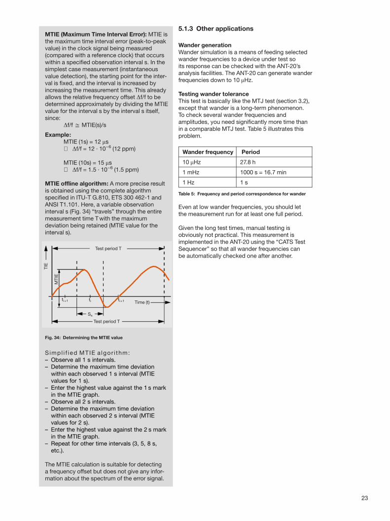
MTIE (Maximum Time Interval Error): MTIE isthe maximum time interval error (peak-to-peakvalue) in the clock signal being measured(compared with a reference clock) that occurswithin a specified observation interval s. In thesimplest case measurement (instantaneousvalue detection), the starting point for the inter-val is fixed, and the interval is increased byincreasing the measurement time. This alreadyallows the relative frequency offset Df/f to bedetermined approximately by dividing the MTIEvalue for the interval s by the interval s itself,since:

Df/f % MTIE(s)/s

Example:MTIE (1s) = 12 ms⇒ Df/f = 12 ´ 10±6 (12 ppm)

MTIE (10s) = 15 ms⇒ Df/f = 1.5 ´ 10±6 (1.5 ppm)

MTIE offline algorithm: A more precise resultis obtained using the complete algorithmspecified in ITU-T G.810, ETS 300 462-1 andANSI T1.101. Here, a variable observationinterval s (Fig. 34) ªtravelsº through the entiremeasurement time Twith the maximumdeviation being retained (MTIE value for theinterval s).

S impl i f ied MTIE a lgor i thm:± Observe all 1 s intervals.± Determine the maximum time deviation

within each observed 1 s interval (MTIEvalues for 1 s).

± Enter the highest value against the 1 s markin the MTIE graph.

± Observe all 2 s intervals.± Determine the maximum time deviation

within each observed 2 s interval (MTIEvalues for 2 s).

± Enter the highest value against the 2 s markin the MTIE graph.

± Repeat for other time intervals (3, 5, 8 s,etc.).

The MTIE calculation is suitable for detectinga frequency offset but does not give any infor-mation about the spectrum of the error signal.

5.2 Offline wander analysis

The MTIE/TDEV analysis software considerablyextends the wander analysis capabilities describedin the previous section.

5.2.1 Test principle

Offline wander analysis is based on TIE samplesgathered during a wander measurement. Two fileformats are accepted: The ANT-20's file format andthe *.csv file format (compatible with MS Excel).

Using the recorded TIE samples, an MTIE/TDEVanalysis can be performed to ETSI Recom-mendation ETS 300 462 (as per ITU-T G.810,G.811, G.812, G.813). The frequency offset anddrift rate are also computed to ANSI T1.101(see also p. 27).

You can install the MTIE/TDEV software on theANT-20 or a separate PC. It computes the MTIEand TDEV curves with the specified algorithms.All tolerance masks are available for evaluationpurposes that are required for qualifying synchron-ization elements (e.g. as per the ANSI, ETSI andITU-T norms). To provide a quick overview, aªsoftware LEDº delivers a PASS/FAIL result. User-specific tolerance masks can also be programmed.

The built-in software simulator makes it easy tosuperimpose sinusoidal, linear or square-wavesignals or even white noise to give a ªvirtualºTIE curve. They can also be evaluated using thesoftware and compared with ªrealº measurementtraces.

5.2.2 Displaying the test results

The offline analysis software has two presentationformats:

TIE analyzerThis mode lets you examine the recorded TIEsamples in greater detail. Zoom functions makeit easier to identify and analyze crucial timesegments. Several TIE measurements can beloaded into the TIE analyzer and compared, e.g.several measurements on the same DUT (Fig. 35).The frequency offset and the drift rate are alsodisplayed. The frequency offset can be eliminated(frequency-offset-compensated TIE display).The zoom function lets you pick a reasonableevaluation interval for MTIE/TDEV offline analysis.

MTIE/TDEV windowThis mode lets you start the MTIE and the TDEValgorithm. Reasonable observation intervals withinthe overall measurement time are used for com-putation purposes, and the results for each intervalare displayed as a point.Various tolerance masks can be inserted whichcharacterize the different quality levels (e.g. PRClevel, SSU level).

24

Fig. 35: The TIE analyzer showing multiple TIE measurements

Fig. 36: MTIE and TDEV analysis, shown here with tolerancemask (passed)

5.2.3 Investigating the phasetransient response

A wander measurement (TIE) is useful for checkingthe phase transient response. However, set theTIE sample rate to 300/s for a larger resolution sothat any fast transients can be detected. Theresolution achieved is 10 times higher than thefigure specified in O.172. The offline analysis soft-ware allows you to investigate the phase transientresponse with even greater precision. You can usethe 200 m function to precisely select and analyzethe time segment.

Besides 24 hour acceptance tests ªin compliancewith O.172, PRC levelº and long-term monitoringwork in combination with a bit error rate test(BERT), investigation of phase transient responseis particularly important. Phase transients ariseat the outputs of synchronized clock generatorsdue to interference to the reference signal, e.g.when the synchronization signal is interrupted orwhen switching between different synchronizationsources. One distinguishes between short-termand long-term phase transient response.

Short-term phase transient responseThis occurs when an impairment causes a switch-over to another reference source for which thesame primary source is the basis (Fig. 37). Afterswitch-over, the phase must settle down to thenew synchronization source, which may last upto 15 s. A maximum clock deviation of 1000 ns isstipulated as the tolerance mask (see ITU-T Rec.G.813).

Long-term phase transient responseThis occurs when the synchronization source islost and the clock generator has to go into holdovermode. Since a frequency offset can last in this caseover a longer time period, the phase deviation overtime is basically unlimited. However, based on themaximum tolerable frequency error in holdovermode, there is a maximum slope of the phasedeviation vs. time (Fig. 38).

The frequency offset of 4.6610±6 may not beexceeded by a SEC. The value is directly displayedin the analysis window.

25

Deviation 51011

TIE

Deviation 51011

Transientregion Time

Fig. 37: Short-term phase transient response

TIE

Deviation 51011

Deviation54.661011

Time

Fig. 38: Long-term phase transient response (ªholdover modeº)

26

Test length T

TIE

ti+1

Sx Time (t)

ti ti+1

Observationinterval

Small interval

s1

H(f)

f0.42s1

RMS value

Medium interval

s2

H(f)

f0.42s2

RMS value

Large intervals3

H(f)

0.42s3

f

RMS value

TD

EV

High-frequency Low-frequency

Components

s1 s2 s3s

Fig. 39: Determining the TDEV value

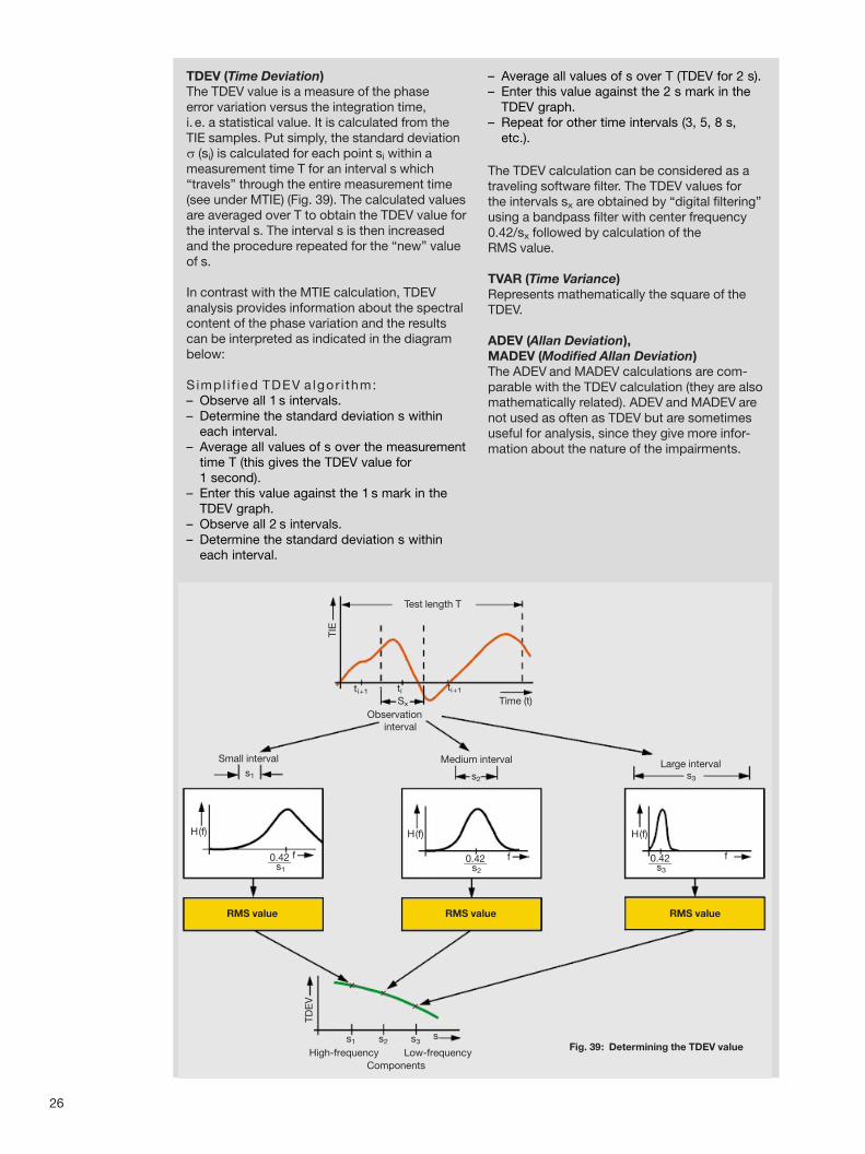
TDEV (Time Deviation)The TDEV value is a measure of the phaseerror variation versus the integration time,i. e. a statistical value. It is calculated from theTIE samples. Put simply, the standard deviations (si) is calculated for each point si within ameasurement time T for an interval s whichªtravelsº through the entire measurement time(see under MTIE) (Fig. 39). The calculated valuesare averaged over T to obtain the TDEV value forthe interval s. The interval s is then increasedand the procedure repeated for the ªnewº valueof s.

In contrast with the MTIE calculation, TDEVanalysis provides information about the spectralcontent of the phase variation and the resultscan be interpreted as indicated in the diagrambelow:

S impl i f ied TDEV a lgor i thm:± Observe all 1 s intervals.± Determine the standard deviation s within

each interval.± Average all values of s over the measurement

time T (this gives the TDEV value for1 second).

± Enter this value against the 1 s mark in theTDEV graph.

± Observe all 2 s intervals.± Determine the standard deviation s within

each interval.

± Average all values of s over T (TDEV for 2 s).± Enter this value against the 2 s mark in the

TDEV graph.± Repeat for other time intervals (3, 5, 8 s,

etc.).

The TDEV calculation can be considered as atraveling software filter. The TDEV values forthe intervals sx are obtained by ªdigital filteringºusing a bandpass filter with center frequency0.42/sx followed by calculation of theRMS value.

TVAR (Time Variance)Represents mathematically the square of theTDEV.

ADEV (Allan Deviation),MADEV (Modified Allan Deviation)The ADEV and MADEV calculations are com-parable with the TDEV calculation (they are alsomathematically related). ADEV and MADEV arenot used as often as TDEV but are sometimesuseful for analysis, since they give more infor-mation about the nature of the impairments.

27

TIE

Offset corrected TIE

Frequencyoffset

Time

Data in

Buffer

f0

f0Data out

Drift rate

TIE

Frequencyoffset

Time

Fig. 40: Buffers are used to compensate for frequencyfluctuations

Fig. 41: Influence of the drift rate and frequency offseton TIE (Time Interval Error)

Fig. 42: In the RMTIE measurement, the frequency offsetis subtracted from the result

Interpreting the MTIE, TDEV, ADEVand MADEV curvesADEV, MADEV and TDEV may yield differentresults depending on the type of interferencesignal (see Table 2, p. 28). As well as the obviouseffects due to frequency offset and drift, thetypical noise processes encountered in oscil-lators are also listed.As the table shows, the MTIE calculation is theonly method described that can detect theimportant (and frequently occurring) case offrequency offset. On the other hand, the TDEVcalculation gives information about frequencydrift or oscillator noise. If, for example, the slopeof the TDEV curve corresponds to the squareroot of s, this indicates phase modulation withwhite noise.Buffers are used in digital switches, synchronouscross-connects and add-drop multiplexers tocompensate for the frequency variations causedby pointer actions. The MTIE value is usefulfor configuring the buffer, i.e. the buffer isdimensioned according to the specified limitvalue for MTIE. If this value is not exceeded itcan be safely assumed that no buffer overflowswill occur and hence frame slips will be absent.

The TDEV, ADEV and MADEV curves cannotbe used to dimension the buffers, but they areuseful for assessing oscillator performance.ETSI 300 462-3 specifies MTIE and TDEV masksfor all synchronization elements (PRC, SEC,SSU, PDH). These indicate the maximum MTIEor TDEV value for each observation interval. Tosummarize:

. MTIE is a measure of the long-termstability of a clock signal,

. TDEV a measure of the short-termstability.

Frequency offset andfrequency drift rateBesides specifying the phase transientresponse (TIE) for switch-over of a clocksource to holdover mode, the standardsalso stipulate maximum values for theªinitial fractional frequency offsetº and theªfrequency drift rateº. The values aredetermined using special algorithms fromANSI T1.101 (see Table 7, p. 28).

MRTIE (Maximum RelativeTime Interval Errors)If during wander analysis the reference is notavailable, e.g. due to spatial separation, theMTIE analysis can have a frequency offsetsuperimposed on it. It is a function of the clockdifference between the signal and the localreference used for measurement. In theRMTIE measurement, the frequency offset issubtracted from the result so that the truewander is displayed.

6 Jitter and wander test equipment

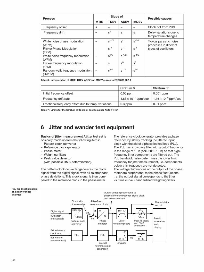
Basics of jitter measurement A jitter test set isbasically made up from the following items:± Pattern clock converter± Reference clock generator± Phase meter± Weighting filters± Peak value detector

(with possible RMS determination).

The pattern clock converter generates the clocksignal from the digital signal, with all its attendantphase deviations. This clock signal is then com-pared to the reference clock in the phase meter.

The reference clock generator provides a phasereference by slowly tracking the jittered inputclock with the aid of a phase locked loop (PLL).The PLL has a lowpass filter with a cutoff frequencyin the range of 1 Hz (ANT-20: 0.1 Hz) so that high-frequency jitter components are filtered out. ThePLL bandwidth also determines the lower limitfrequency for jitter measurement, i.e. componentsbelow this frequency are not detected.The voltage fluctuations at the output of the phasemeter are proportional to the phase fluctuations,i. e. the output signal corresponds to the jittervs. time curve. Standardized weighting filters

28

ProcessSlope of

Possible causesMTIE TDEV ADEV MDEV

Frequency offset s ± ± ± Clock not from PRS

Frequency drift ± s2 s s Delay variations due totemperature changes

White noise phase modulation(WPM)Flicker Phase Modulation(FPM)White noise frequency modulation(WFM)Flicker frequency modulation(FFM)Random walk frequency modulaton(RWFM)

±

±

±

±

±

s-1/2

s-0

s1/2

s

s3/2

s-1

s-1

s-1/2

s0

s1/2

s-3/2

s-1

s-1/2

s0

s1/2

Typical parasitic noiseprocesses in differenttypes of oscillators

Table 6: Interpretation of MTIE, TDEV, ADEV and MDEV curves to ETSI 300 462-1

Stratum 3 Stratum 3E

Initial frequency offset 0.05 ppm 0.001 ppm

Frequency drift rate 4.63610±7 ppm/sec 1.16610±8 ppm/sec

Fractional frequency offset due to temp. variations 0.3 ppm 0.01 ppm

Table 7: Limits for the Stratum-3/3E clock source as per ANSI T1.101

Internalreference clock

generation

Output voltage proportional tophase difference between signal clockand reference clock

Resultevaluationanddisplay

Clock withjitter/wander

Jitter-freereference clock

Digital signal

(with jitterand wander)

Ext. referenceclock input

(for wandermeasurement)

Pattern

Clock

Pattern-clockconverter

PLL

Ext.

Int.Phase

detector

j

U

LP

10 Hz

Lowpass

Jitterweighting filters

HP LP

UIrms

Peak-to-peakand RMSevaluation

Demodulatoroutput

MTIE

PLLTIE

UIpp

Fig. 43: Block diagramof a jitter/wanderanalyzer

connected after this (see below under ªJitterweightingº) limit the frequency spectrum of thejitter signal. The positive and negative peak valuesof the filtered signal are measured (peak-to-peakevaluation) and displayed as the jitter result (inUIpp or alternatively in RMS). The filtered signal isavailable at a demodulator output for furtherexternal processing. Further time- and frequency-domain analysis of the jitter is thus possible, e. g.using an oscilloscope, a selective level meter or aspectrum analyzer.

Jitter weightingCombinations of high-pass and low-pass filtersweight the detected jitter signal with regard to itsspectral content. The filter combinations for thevarious transmission interfaces are specified inthe relevant standards (see Appendix, Table 3:ªStandards for jitter and wanderº). Jitter analyzersare therefore equipped with an appropriateselection of highpass and lowpass filters. Byselecting certain frequency ranges from the jitterspectrum, conclusions can be drawn regardingthe frequencies causing the observed problems.

Jitter generatorA jitter generator is needed for measuring jittertolerance and the jitter transfer function. The jittermodulation generator and jitter modulator (phasemodulator) circuits generate a clock signal at thedesired bit rate with defined jitter. This clock signalis used to run the pattern generator that producesthe digital signal. Special stressing signals (pseudo-random noise, sawtooth, etc.) can be fed to theexternal modulator input.

Basics of wander measurementWander measurement basically operates accordingto the same principles as jitter measurement. Anexternal reference clock must be used instead of

the internally generated reference clock, sincephase variations of close to 0 Hz are to bemeasured. If this is implemented using a PLL, thenthe cutoff frequency of the lowpass filter must beas low as possible. The lower the cutoff frequency,then the longer the settling time obtained. Forexample, at a cutoff frequency of 0.0001 Hz, asettling time of several hours is obtained, which isentirely unpractical.

O.171 and 0.172: Recommendations and deviceproperties for jitter/wander measurementAdopted in 1999, ITU-T Recommendation O.172 isentitled ªJitter and Wander Measuring Equipmentfor Digital Systems which are Based on theSynchronous Digital Hierarchy (SDH)º. This newRecommendation takes its place alongside themuch older O.171 governing jitter and wandermeasurements on PDH systems. O.172 isprimarily oriented towards SDH, but it alsoconsiders the interfaces of PDH tributaries.The new Recommendation defines instrumentproperties for measuring and generating jitterand wander. Note that O.172's requirements formeasurement accuracy are in some casesconsiderably tougher than those of O.171. Theweighting filters so critical to measurement are alsoclearly described (see section ªJitter weightingº).New test applications required by the newsynchronous technology are also described (e.g.pointer jitter). Table 8 shows the main differencesbetween O.171 and O.172.

29

20dB

/dec

.

20dB

/dec

.

60dB

/dec.

f1 f2Df23

f3 Frequency

Df13

Am

plit

ud

e

Jitterdetector

Bandpassf1 ± f3

Df13

Df23Bandpass

f2 ± f3

Measu

red

jitte

ram

plit

ud

ein

UI p

p

HP1 HP2 LP

STM-1/OC-3 500 Hz 65 kHz 1,3 MHz

STM-4/OC-12 1 kHz 250 kHz 5 MHz

STM-16/OC-48 5 kHz 1 MHz 20 MHz

Fig. 44: Jitter measurement filters for SDH/SONET bit rates

O.171 O.172

Interfaces Electrical interfacesup to 140 Mbit/s(PDH only)

Electrical and optical inter-faces up to 10 Gbit/s (PDH,SDH, SONET)

Jitter meter,frequency range

10 Hz to 3.5 MHz 10 Hz to 20 MHz(at 2.5 Gbit/s)

Jitter meter,weighting filters

More precise filter definition

Jitter meter,amplitude range

Up to 10 UIpp Increased meas. range,e.g. 200 UIpp for STM-4

Jitter meter,intrinsic error(fixed component)

e. g. 0.085 UIpp at140 Mbit/s

0.025 to 0.05 UIpp

Jitter generator,frequency range

Up to 3.5 MHz Up to 20 MHz(up to 2.5 Gbit/s)

Pointer jitter testapplication

None

Description of test require-ments, pointer test sequences

Wander meter,sampling rate (TIE)

430 Hz

Wander meter,accuracy

+5% (variable component)+2.5 ns (fixed component) forsmall observation intervals

MTIE/TDEValgorithm

Description with accuracyrequirements

Wander generator,amplitude range

53000 UI 5230400 UI

Wander generator,frequency range

412 mHz at 2 Mbit/s 412 mHz at all rates

Table 8: Comparisonbetween O.171 andO.172

Appendix: Standards for jitter and wander

To allow problem-free interconnection of differentnetwork elements in a telecommunications net-work, it is necessary to satisfy maximum jitter andwander amplitude criteria at the interfaces. On theother hand, inputs must tolerate a certain amountof jitter and wander. The accumulation of jitter in a

chain of regenerators must be limited by com-pliance with jitter transfer functions. This is thereason behind the requirements stipulated for alldigital hierarchy levels in the standards of theITU-T, ANSI and ETSI.

30

Table 1: Outputjitter requirements fornetwork interfaces

Networkinterface

Standard Bit rate Jitter limits

Wide-band jitter/UIpp High-band jitter/UIpp

SDH transport ITU-T G.825ETSI EN 302 084

STM-1e 1.5 0.075

STM-1 1.5 0.15

STM-4 1.5 0.15

STM-16 1.5 0.15

STM-64 1.5 0.15

SONET transport ANSI T1.105.03Bellcore GR-253

OC-1 1.5 0.15

OC-3 1.5 0.15

OC-12 1.5 0.15

OC-48 1.5 0.15

PDH transport ITU-T G.823ETSI EN 302 084

2048 kbit/s 1.5 0.2

8448 kbit/s 1.5 0.2

34368 kbit/s 1.5 0.15

139264 kbit/s 1.5 0.075

ANSI T1.102Bellcore GR-499ITU-T G.824

1544 kbit/s 5 0.1

6312 kbit/s 3 (NOTE 1) 0.1

44736 kbit/s 5 0.1

Synchronization ITU-T G.823ETS 300 462-3

2048 kbit/s PRC 0.05 -

2048 kbit/s SSU 0.05 -

2048 kbit/s SEC 0.5 0.2

2048 kbit/s PDH 1.5 0.2

ANSI T1.101 1544 kbit/s 5 0.1

Equipment Standard Bit rate Jitter limits

Wide-band jitter/UIpp High-band jitter/UIpp

SDH (TM, ADM, DXCetc.)

ITU-T G.813ETS 300 462-5

STM-1 0.5 0.1

STM-4 0.5 0.1

STM-16 0.5 0.1

ANSI T1.105.03 OC-1 0.01 UIrms (12 kHz) Ð

OC-3 0.01 UIrms (12 kHz) Ð

OC-12 0.01 UIrms (12 kHz) Ð

OC-48 0.01 UIrms (12 kHz) Ð

Bellcore GR-253 OC-1 0.1 (0.01 UIrms) Ð

OC-3 0.1 (0.01 UIrms) Ð

OC-12 0.1 (0.01 UIrms) Ð

OC-48 0.1 (0.01 UIrms) Ð

SDH regenerators ITU-T G.783NOTE 1

STM-1 0.3 0.1

STM-4 0.3 0.1

STM-16 0.3 0.1

PRC clock ITU-T G.811ETS 300 462-6

2048 kbit/s 0.05 Ð

1544 kbit/s 0.015 Ð

SSU clock ITU-T G.812ETS 300 462-4

STM-1e 0.5 0.075

STM-1 0.5 0.1

STM-4 0.5 0.1

STM-16 0.5 0.1

2048 kbit/s 0.05 Ð

1544 kbit/s 0.05 Ð

PDH ITU-T G.735 2048 kbit/s 0.05 Ð

ITU-T G.742 8448 kbit/s 0.05 Ð

ITU-T G.751 34368 kbit/s 0.05 Ð

139264 kbit/s 0.05 Ð

Table 2: Outputjitter requirements forequipment

NOTE 1: Revised DraftG.783 (10/98)

NOTE 1: In DraftRevised G.824: 5 UIpp

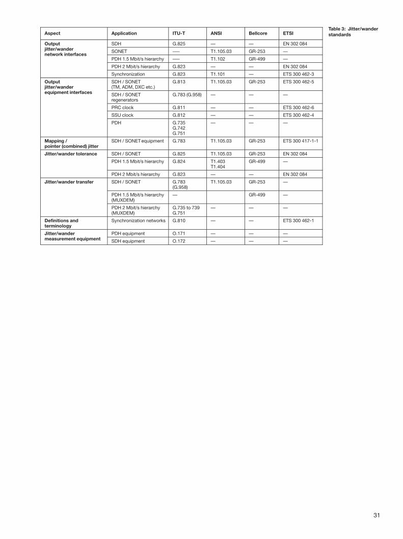
31

Aspect Application ITU-T ANSI Bellcore ETSI

Outputjitter/wandernetwork interfaces

SDH G.825 Ð Ð EN 302 084

SONET б T1.105.03 GR-253 Ð

PDH 1.5 Mbit/s hierarchy б T1.102 GR-499 Ð

PDH 2 Mbit/s hierarchy G.823 Ð Ð EN 302 084

Synchronization G.823 T1.101 Ð ETS 300 462-3

Outputjitter/wanderequipment interfaces

SDH / SONET(TM, ADM, DXC etc.)

G.813 T1.105.03 GR-253 ETS 300 462-5

SDH / SONETregenerators

G.783 (G.958) Ð Ð Ð

PRC clock G.811 Ð Ð ETS 300 462-6

SSU clock G.812 Ð Ð ETS 300 462-4

PDH G.735G.742G.751

Ð Ð Ð

Mapping /pointer (combined) jitter

SDH / SONET equipment G.783 T1.105.03 GR-253 ETS 300 417-1-1

Jitter/wander tolerance SDH / SONET G.825 T1.105.03 GR-253 EN 302 084

PDH 1.5 Mbit/s hierarchy G.824 T1.403T1.404

GR-499 Ð

PDH 2 Mbit/s hierarchy G.823 Ð Ð EN 302 084

Jitter/wander transfer SDH / SONET G.783(G.958)

T1.105.03 GR-253 Ð

PDH 1.5 Mbit/s hierarchy(MUXDEM)

Ð GR-499 Ð

PDH 2 Mbit/s hierarchy(MUXDEM)

G.735 to 739G.751

Ð Ð Ð

Definitions andterminology

Synchronization networks G.810 Ð Ð ETS 300 462-1

Jitter/wandermeasurement equipment

PDH equipment O.171 Ð Ð Ð

SDH equipment O.172 Ð Ð Ð

Table 3: Jitter/wanderstandards

Wandel&Goltermann Worldwide

North America

CanadaWavetek Wandel GoltermannCanada Inc.21 Rolark DriveScarborough, Ontario M1R3B1Tel. +1-416 2917121Fax +1-416 291 2638

USAWandel & Goltermann Inc.P.O. Box 13585Research Triangle Park,NC 27709-3585Tel. +1-919-941-5730Fax +1-919-941-5751

MexicoWandel & Goltermann de Me xicoS.A. de C.V.San Francisco No. 6Col. Del ValleMe xico D.F.CP 03100 Me xicoTel. +52-5 543 6644Fax +52-5 543 8660

Latin America

Argentina/UruguayWandel & Goltermann S.A.MontanÄ eses 25991428 Buenos AiresArgentinaTel. +54-11 4784 4700Fax +54-11 4786 7917

Brazil/Chile/Peru/Bolivia/ParaguayWandel & GoltermannInstrumentacË aÄ o Ltda. & Cia.Av. Eng. Luis Carlos Berrini,936-9. andar04571-000 SaÄ o Paulo, SPBrazilTel. +55-11 5503 3800Fax +55-11 5505 1598

Europe

AustriaCIS Countries, East and SoutheastEurope, Iran, Turkey, PakistanWavetek Wandel GoltermannAustria GmbHPostfach 13Elisabethstraûe 36A-2500 BadenTel. +43-22 52 85 521-0Fax +43-22 52 80 727

BeneluxWavetek Wandel GoltermannBenelux BVPostbus 1575NL-5602 BN EindhovenTel. +31-40-267 97 00Fax +31-40-267 97 11

FinlandWandel & Goltermann ABTekniikantie 12FIN-02150 EspooTel. +358-(0)9-4354 3199Fax +358-(0)9-455 1522

FranceWandel & Goltermann France46 bis, rue Pierre CurieB.P. 10Z.I. Les Gaà tinesF-78373 Plaisir Ce dexTe l. +33-(0)1 30 81 50 50Fax +33-(0)1 30 55 87 75

GermanyWavetek Wandel GoltermannGmbH & Co.VertriebsgesellschaftP.O.Box 11 55D-72794 Eningen u.A.Tel. +49-7121 862222Fax +49-7121 861222sales.germany@wwgsolutions.com

ItalyWandel & Goltermann S.R.L.Communications Test SolutionsVia Pomponazzi 25I-20 141 MilanoTel. +39-02 895 12381Fax +39-02 895 11780

NorwayWandel & Goltermann ABPostboks 134, SkùyenHovfaret 13N-0212 OsloTel. +47-22-504090Fax +47-22-504025

Russia, CISWandel & Goltermann OOO1st Neopalimovskiy Pereulok 15-7/4th FloorRF-119121 MoscowTel. +7-095-797 29 50Fax +7-095-797 29 50

Spain/PortugalWandel & Goltermann S.A.c/Arturo Soria no 343 - 3o

E-28033 MadridTel. +34-91-383-9801Fax +34-91-383-2263

SwedenWandel & Goltermann ABBox 6044Ellen Keys Gata 60S-129 06 HaÈ gerstenTel. +46-8-449 48 00Fax +46-8-449 48 39

SwitzerlandWandel & Goltermann (Schweiz) AGPostfach 779Morgenstrasse 83CH-3018 Bern 18Tel. +41-31 996 44 11Fax +41-31 996 44 22

United KingdomWandel & Goltermann Sales Ltd.Portland House, Aldermaston ParkAldermaston, Berkshire RG7 4HREnglandTel. +44-1189 409200Fax +44-1189 409210e-mail: wguk.help@wago.de

East and South East Europesee Austria

Africa

Wandel & Goltermann GmbH & Co.VertriebsgesellschaftP.O.Box 1155D-72794 Eningen u.A.Tel. +49-7121-86 11 83Fax +49-7121-86 21 55export.germany@wwgsolutions.com

Asia

Middle East see Africa

South East Asia see Australia

CIS Countries/Iran/Turkey/Pakistansee Austria

ChinaWandel & Goltermann Pty. Ltd.Beijing OfficeSuite 1608 Corporate SquareNo. 35 Jinrong Street, Xicheng DistrictBeijing 100032Peoples Republic of ChinaTel. +86-10-8809 1288Fax +86-10-8809 1298

Hong KongWavetek Wandel GoltermannHong Kong Ltd.Rm 1901-2 Jubilee Centre18 Fenwick StreetWanchai, Hong KongTel. +852-2528-6283Fax +852-2529-5593

IndiaWandel & Goltermann Pvt. Ltd.R. K. Khanna Tennis StadiumAfrica AvenueNew Delhi 110029Tel. +91-11-619 6420Fax +91-11-619 6190

JapanWandel & Goltermann K.K.Kyoritsu Shin-Yokohama Bldg. 6F2-15-12 Shin-YokohamaKouhoku-kuYokohama, 222-0033JapanTel. +81-45-473-9501Fax +81-45-473-9812

Republic of KoreaWavetek Wandel GoltermannKorea Ltd.1st Fl., Yehsung Bldg.150-30 Samsung-dong, Kangnam-ku,Seoul 135-091, KoreaTel. +82-2-563 2236/7Fax +82-2-563 2239

SingaporeWavetek Asia-Pacific Pte Ltd438B Alexandra RoadAlexandra Technopark Hex 06-07Singapore 119968Tel. +65-377-3003Fax +65-377-3033

Australia and Pacific Region

AustraliaWavetek Wandel GoltermannAsia Pacific Pty. Ltd.P.O. Box 419World Trade CentreMelbourne, Victoria 3005AustraliaTel. +61-3-9690 6700Fax +61-3-9690 6750

New ZealandWandel & Goltermann Pty. Ltd.P.O. Box 10 418The TerraceWellingtonNew ZealandTel. +64-4-4952290Fax +64-4-4952292

For all other countries(not listed) please contact:

Wandel &Goltermann GmbH &Co.Elektronische MeûtechnikMarketing InternationalPostfach 12 62D-72795 Eningen u.A.Tel. +49-7121-86 16 16Fax +49-7121-86 13 33E-mail: info@wwgsolutions.comhttp://www.wwgsolutions.com

Subject to change without notice ± Order no. TP/EN/A071/0799/AEPrinted in Germany