Leadership Effects: School Principals and StudentOutcomes∗

Michael Coelli† and David A. Green‡

19 August 2011

Abstract

We identify the effect of individual high school principals on graduation rates and En-glish exam scores using an administrative data set of grade 12 students in BC Canada. Manyprincipals were rotated across schools by districts, permitting isolation of the effect of prin-cipals from the effect of schools. We estimate the variance of the idiosyncratic effect ofprincipals on student outcomes using a semi-parametric technique assuming the effect istime invariant. We also allow for the possibility that principals take time to realize their fulleffect at a school.

JEL codes: I20, I21

Keywords: educational economics, efficiency, human capital

∗The statistical analysis presented in this document was produced from administrative micro-data provided bythe British Columbia Ministry of Education. The interpretation and opinions expressed are our own and do notrepresent those of the BC Ministry of Education. We are indebted to David Harris for assistance and advice. Thanksalso to seminar participants at the University of British Columbia, University of Melbourne, Monash, UNSW andACE Adelaide 2009.

†Department of Economics, The University of Melbourne‡Department of Economics, University of British Columbia and Research Fellow, Institute for Fiscal Studies,

London

1 Introduction

Years after the Coleman Report (1966) on schooling in the United States, there remains consid-

erable debate on whether schools can actually improve student outcomes.1 The Report’s authors

claimed that measurable school inputs, such as spending per student, pupil-teacher ratios, and the

education and experience of teachers, had no significant effect on student outcomes, once student

family background and peer effects were controlled for. However, more recent research focus-

ing on unobservable teacher “quality” (or, teacher “fixed effects”) finds that teachers matter,2

supporting claims in parts of the education literature. In this paper, we employ the techniques

from the teacher fixed effect literature to examine a less studied part of the schooling production

function: principals.

School principals may affect student outcomes through a variety of paths. As school lead-

ers, they have considerable influence on aspects of the school such as teacher supervision and

retention, introducing new curricula (in some cases) and teaching techniques, student discipline,

and student allocation to teachers and classes. Education scholars have grouped these pathways

into: (1) purposes and goals, (2) structure and social networks, (3) people, and (4) organiza-

tional culture (Hallinger and Heck(1998)). Research in that literature has examined the impact

of principals within a wider agenda of attempting to identify the attributes of high achieving

or effective schools and has found mixed results concerning principal effects (Hallinger and

Heck(1998)). However, most of the education literature research is based on surveys of teacher

perceptions about leadership and school conditions, raising concerns about endogeneity and mis-

measurement.3 As we will discuss momentarily, there is now a small but growing economics

1The exchange between Krueger (2003) and Hanushek (2003) highlights the extent of this debate.2This research includes, among others, Goldhaber and Brewer (1997), Park and Hannum (2002), Rowan et al

(2002), Uribe et al (2003), Rockoff (2004), Nye et al (2004), Rivkin et al (2005), Kane et al (2008), Aaronson etal (2007), Konstantanopoulos (2007), Leigh (2007) and Koedel (2008). Older teacher fixed effect studies includeHanushek (1971), Armor et al (1976) and Murnane and Phillips (1981).

3For example, in the survey used in Leithwood and Jantzi (1999) teachers are asked to rate how strongly theyagree with the statement, “Our school administrators have a strong presence in the school.”

1

literature on principal effects. We add to that literature by providing estimates employing data

variation from principal changes where a significant portion of those changes are due to school

district principal rotation practices. We also explicitly introduce the possibility of quite flexible

principal tenure effects into the measurement of principal impacts. We allow for tenure effects to

be different in both size and sign across principals and schools, rather than imposing the standard

technique of only allowing the same tenure profile for all principals. This is particularly impor-

tant in the leadership setting, as principals new to a school could be of higher or lower quality

than the principals that preceded them.

We estimate the effect of individual school principals on student high school graduation

probabilities and grade 12 provincial final exam scores employing a unique administrative dataset

from the Canadian province of British Columbia. School districts in British Columbia rotate

high school principals across schools, with this being a stated policy in some districts and a

reflection of ongoing principal turnover in others. Taking advantage of this, we employ turnover

of principals within schools over time to identify their effects on student outcomes purged of any

fixed school, neighborhood or stable peer group effects. We use administrative information on

all students entering grade 12 in British Columbia (BC) over the 1995 to 2004 period. Unlike

in many U.S. jurisdictions that have received attention in recent years (see e.g., Jacob and Levitt

(2003), Figlio (2006), McNeil et al. (2008)), there are no direct incentives for principals to meet

specific graduation rate or exam score targets for their schools. School funding is based on a

fixed formula that is mainly a function of the number of students and neither it nor principal

compensation is based on student outcomes. This is important because, as the U.S. literature

highlights, in situations with clear funding and pay incentives based on student outcomes, there

is an incentive for principals to “game” outcomes so that a person who appears to be an effective

principal may just be one who is a good strategic player. We don’t claim that cheating is entirely

absent among this set of principals, since they are at least being implicitly evaluated on the

2

outcomes in their schools, but the lack of clear incentives suggests this may not be a primary

issue in our data.

Our empirical strategy has two main components. First, we adapt the technique used by

Rivkin et al (2005) in their study of teacher effects to identify a lower bound estimate of the

variance in the quality of individual school principals. We refer to “quality” as the impact a prin-

cipal has on student outcomes. In essence, the idea behind the estimator is that if principals have

individual effects on school outcomes, then the variance of those outcomes should be greater in

schools which have more principals over a given time period. Unlike Rivkin et al (2005), we

do not follow students longitudinally and so cannot control for individual student fixed effects.

Thus, our identification requires that principals were not rotated across schools in response to

changes in the quality of students, and that students do not sort themselves across schools in

response to principal changes. Importantly, our estimation technique does allow for principal

allocation based on long-run average student quality in the school; just not on changes in stu-

dent quality over time. This technique assumes that individual principals have an immediate and

constant effect on the schools that they lead. The main benefit of this strategy is that it provides

a direct statistical test of whether there are observable differences in student outcomes across

principals, that is, a test of whether there is positive variance in the quality of school principals.

The approach, in fact, yields a lower bound estimate of the variance of principal effects under the

assumptions just mentioned: no sorting of students in response to principal assignments; linarly

additive school and principal fixed effects; and no changes in principal effects with tenure at the

school.

In the second component of our empirical strategy, we estimate a simple dynamic model

of the effect of school principals on student outcomes. This strategy allows for a potentially

cumulative effect of school principals on schools over time. A glance at the routes through

which principals are hypothesized to influence outcomes suggests that it may take a number of

3

years for them to have a measurable influence on student outcomes. If we do not take this into

account then an approach like our first, semi-parametric technique may under-estimate the true

full impact a principal could have on a school (given enough time). In particular, in a school in

which the principal turned over every year, no principal may be able to put his or her “mark” on

the school. The result would be a lower variance in outcomes over time within the school than

one would witness if each principal’s full effect were realized. We interpret the second approach

as relaxing the assumption of immediately-evident, time-invariant principal effects in the first

approach. This advantage comes at the cost of assuming a parametric form for the principal

tenure profile. As before, it requires assumptions of no experience effects and no student sorting.

In both the time invariant effect and dynamic estimation strategies, we estimate the effect of

individual school principals on student outcomes after first controlling for aggregate time effects

and a number of individual student and neighborhood characteristics.

Our analysis adds to a small but growing number of economic analyses of school principals.

Gates et al (2006) found principals were more likely to leave schools with higher proportions

of minority students. Cullen and Mazzeo (2007) find evidence that higher school performance

is followed by higher pay for the principal in Texas schools. This does not appear to be feasi-

ble in the BC system, where principal incomes are often determined on a pre-set grid.4 Branch

et al (2008) find small tenure and experience effects on student performance for principals in

Texas schools. They also find large variation in principal fixed effects, using switching princi-

pals only in identification. Lavy (2008) investigates the effect of raising school principal pay on

high school student outcomes in Israel, and finds sizable effects on high school graduation and

matriculation exam scores. Clark et al (2009), using school data for students in grades 3 through

8, find significant principal experience effects, but no education effect and mixed training effects

in New York City schools. Miller (2009) finds that a downturn in student performance precedes

4We discuss principal compensation in BC in the next section of the paper.

4

a principal departure, and that principal transition lowers teacher retention in North Carolina

schools. Cullen and Mazzeo (2007), Branch et al (2008), Clark et al (2009) and Miller (2009)

all found higher principal turnover occurred in low performing schools, and that switching prin-

cipals are more likely to go to higher achieving schools.5

We add to this growing literature in a number of ways. To begin, our data contains a par-

ticularly large number of principal switches, which is the basis for our identification strategy.

Second, we use that variation to provide a semi-parametric estimate of the variance of principal

effects, after controlling for permanent school specific effects to address the issue identified in

the existing literature of better principals being sorted to specific types of schools. Third, we

estimate a dynamic model that allows for lags in the effect that principals may have on student

outcomes, as a new principal may take several years to have their full impact on a school. Our

dynamic model can allow for quite flexible potential tenure effects, and adds to earlier findings

that principal tenure or experience matter for student outcomes.

Our results suggest that there is sizable heterogeneity in school principal quality, particularly

in affecting the grade 12 English exam scores of students. Specifically, getting a principal who

is one standard deviation better in the principal effects distribution implies that graduation rates

will be higher by 2.6 percentage points (or, roughly, a third of a standard deviation of the cross-

school graduation rate distribution) and English exam scores will be higher by 2.5 percentage

points (roughly equivalent to a standard deviation) if principals are given time to fully “make

their mark” on the school. Our empirical strategies, however, come at the expense of not being

able to identify the particular pathways through which principals affect student outcomes nor the

strategies employed by effective principals. Thus, this paper represents a first step toward a more

complete understanding of the role principals play in affecting student outcomes.

The outline of this paper is as follows. In section 2, we describe the BC school environment.

5Authors et al (2007) employed school principals as instruments for high school graduation when investigatingthe effect of graduation on subsequent welfare use for youth from welfare backgrounds.

5

We outline the empirical models in section 3 and describe the administrative data we employ in

section 4. We provide semi-parametric lower bound estimates of the variance of principal quality

assuming principals have a constant immediate effect on schools in section 5 and estimates from

our dynamic model of school principal effects in section 6. Section 7 concludes.

2 The Environment

The data we employ is BC Ministry of Education administrative data on all youth enrolled in

grade 12 in public schools at the start of November in the period 1995 to 2004. Private schools

are not a substantial factor in BC, with only 7.5% of grade 12 students attending private high

schools in 2002 (Authors et al (2007)). Students in BC obtain a high school diploma if they

complete 80 credits at the grade 10 or higher level, including a certain number of required credits,

and with 16 credits being at the grade 12 level. A typical student enters grade 12 having to pass

five more courses (worth 20 credits) to graduate. The only required grade 12 level course is

English 12. In June of the grade 12 year, students are required to take a province-wide exam in

English 12 which counts for 40% of their English grade. Students do not have to pass the exam

in order to pass their English course. We have the student scores on the provincial English exam

for those who took it and we know whether a student has obtained their graduation diploma by

the end of our data period (2005), though we focus on graduation within one or two years of their

registration in grade 12 in order to maintain comparability across years. Approximately 82% of

the students in our data graduate within 2 years of entering grade 12, indicating that a substantial

proportion drop out even after starting grade 12. A Canadian version of the GED is available for

students who drop out of high school but it is not a widely used option.6

As mentioned in the introduction, the expansion of high stakes student assessments in the

6In Statistics Canada surveys, approximately 7.5% of 20 to 24 year old individuals report that they have notcompleted high school in BC in our period, though this is likely to be something of an understatement of the truedrop-out level (Bowlby (2005)).

6

U.S. has led to investigations of whether the associated incentives have led to various forms of

questionable responses. These range from “teaching to the test” to outright cheating on test com-

pletion and putting weak students in categories where they do not get assessed. While some of

these responses appear to occur at the teacher level (Jacob and Levitt (2003)), others are at the

level of principals or other administrators (e.g. Figlio (2006), McNeil et al (2008)). Principal

cheating on the outcomes we examine seems unlikely in BC for several reasons. First, both

principal compensation and school resources are set according to provincial guidelines based on

factors such as school size, but neither are linked to student outcomes (BC Ministry of Educa-

tion (2008), Beresford and Fussell (2009)). Second, the grade 12 provincial English exam is

marked centrally, leaving little opportunity for local manipulation. Third, there is no opportunity

for principals to manipulate enrolment to alter graduation rates since students are guaranteed

enrolment in their ”catchment area” school.

As we will see in the following sections, principal rotation across schools is a key input into

our identification strategy. Principal rotation is determined at the school district level in BC.

There are 55 school districts, each having a school board and a superintendent (the chief admin-

istrative officer). The number of high schools in a district ranges from a low of 1 to a high of 18.

Each district has written policies posted on their web site. In 14 districts, corresponding to 37

percent of all high schools, principal rotation is explicitly mentioned in their district policies. The

average number of high schools in districts with policies on principal rotation is 5.8 compared

to 3.5 for those without, implying that it is the larger districts that tend to have explicit poli-

cies. For example, the Vancouver School Board (the largest district) has a policy which states,

”It is the practice of the Board to transfer principals approximately every five years, although

this period may be extended depending on special circumstances such as a principal nearing re-

tirement”. Other districts have similar policies, with stated minimum and maximum times until

rotation but also allowing some leeway in the application of the policy. In the districts without

7

explicit policies, some have policy statements declaring that Superintendents have power over

these decisions and some have no statement at all. We contacted several of the smaller districts

without explicit policies and were told that they simply had too few schools to have a regularized

rotation system. The average number of years that we observe a principal leading a school in our

data is 3.3 in districts with policies and 3.6 in districts without, so the policies do lead to more

principal changes.7 However, even districts without explicit policies have a considerable amount

of turnover and rotation. Thus, there is good variation for us to work from.

The province of BC has one large city (Vancouver and its surrounding area), one smaller

city (Victoria), and a wide rural expanse. Schools in the cities may be able to attract a wider

pool of principal applicants due to the better amenities on offer to residents, so such schools

may be able to hire on average a better quality of principal. Our estimation strategies (detailed

below) employ within school variation in outcomes over time only, to avoid attributing school

differences to principals. Variation in principal quality may in fact be larger across schools than

within schools over time. As a result, our estimates of principal effectiveness are likely to be a

lower bound on the effect of principals on schools.

As noted above, explicit principal rotation policies were more common in school districts

with more schools. Such districts are more common in the cities. As a result, there were some

differences in student and school attributes between schools with and without rotation policies.

Students in schools with explicit principal rotation policies were more likely to be English as a

Second Language (ESL) students, less likely to be of First Nation background, more likely to

live in wealthier and more educated neighbourhoods, and more likely to be in larger schools.

Note, however, that the student outcomes we investigate were only marginally better in schools

7Note that these average years leading a school numbers understate the total number of years principals leadschools in BC as many of our observed principal spells are censored due to the ten year data window we observe.Employing standard survival time estimation techniques to deal with right censored spells (left censored spellswere dropped), the estimated mean number of years a principal leads a school is 4.6 years in districts with rotationpolicies, and 6.6 years in the remaining districts.

8

with principal rotation policies.

3 Empirical Models of Student Outcomes

3.1 General Model

We begin by setting out a simple heuristic model of high school graduation with the intention of

using it to discuss estimation issues. Many of the points raised in this discussion will carry over

to consideration of exam scores and we will return to this outcome at the end of this section.

We think of the graduation outcome as the reflection of an optimizing decision by the student

in which he or she compares the effort costs of completing courses to the expected benefits.

Inputs from families and schools can reduce the effort (or the dis-utility of the effort) required

to get a passing grade. Families, peers and neighbors can all have effects on perceptions of

benefits from graduation. Principals may have impacts through their effectiveness in marshalling

school resources, including teachers, and through motivation. Based on this, consider a simple

regression in which an indicator for whether an individual i in cohort t at school s graduates from

high school, Gist, is written as a linear function of school (δ), principal (θ) and individual (γ)

effects, plus a random error term (υ), assumed to be independent of the other three components.

Gist = δs + θst + γist + υist (1)

We will estimate this equation using two different assumptions about how θ varies over time,

set out in the two subsections that follow. Our goal is to identify these principal effects, and

we discuss the assumptions required for identification in detail below. The school fixed effect

will capture features of the school that are persistent within our ten year time period. Thus, this

will include features such as persistently high levels of parental involvement and persistently

high or low peer quality as well as physical attributes of the school. It is worth noting that with

9

school operating and capital funding coming from the province based on fixed formulas, there

is little room for persistent differences in most school resources (though, an effective principal

may be one who is better at finding ways to get extra resources from the province). We view the

individual effect, γ, as reflecting a combination of: neighborhood (where the neighbuorhood is

smaller than the school catchment area); demographic factors such as gender, aboriginal status

and language spoken at home; parental inputs of time and other resources; impacts of peers; and

individual cognitive and non-cognitive abilities.8 In section 4, we describe a set of covariates

that we include in order to capture some of these factors. The υ term also includes all other

unobserved factors affecting graduation such as shocks to the school environment.9

The key identification issues we face involve separating principal effects from general school

effects, and from variation in the quality of the student cohorts that enter the school during their

regime. We address the first issue by using school fixed effects. Thus, our identification will

come from variation within schools which have multiple principals in our data period. Systematic

assignment of principals with particular characteristics to perennially better schools is not a

problem within this identification strategy. Since all principals within a given school would be

assigned based on the perennial quality of the school, comparisons among them will not reflect

any systematic bias. Similarly, students who move in order to attend perennially better schools

are not a problem. Problems would arise, however, if principals were assigned to schools based

on changes in the quality of students across cohorts or if students change schools in order to get

a specific principal. In either case, what we interpret as a principal effect in improving student

outcomes could really be a selection effect. We have no way to test whether these selection

8All of these factors have been the focus of a considerable body of research on what affects schooling outcomes.See for example, Carneiro et al. (2003), Todd and Wolpin (2003), and Author et al. (2009) on the impacts ofabilities, family background and peers on graduation and test score outcomes. Foley (2010) examines the impactof neighborhoods on youth educational outcomes in Canada, controlling for school and family inputs. Friesen andKrauth (forthcoming) examine the important issue of peer effects on aboriginal student outcomes in BC.

9The assumption that υ is independent of the other factors is innocuous. It means that if there are shocks that arecorrelated with a given principal, we incorporate those into the principal effect. What is left in the error, then, arethe remaining, orthogonal shocks.

10

mechanisms are at work. However, apart from students attending specialized programs, there is

very little tendency for students to attend schools outside their catchment area, and we are not

aware of any information indicating that principals are assigned based on anticipated changes in

cohort quality. Thus, we believe that the key identifying assumption of no systematic selection

with respect to changes in cohort quality is reasonable.

It is worth noting that we examine graduation rates for students who register in grade 12 in

the fall of a school year. The legal school leaving age is 16 in BC and there is dropping out

in grade 11. Thus, the students in our sample are a select group. This may have an impact on

our results if principals differ in when they have an impact on students. Thus, a principal who is

good at keeping students from dropping out in grade 11 but doesn’t maintain that impact in grade

12 may have a relatively low graduation rate by our measure. We have no way to address this

issue and so must assume that a principal who is able to get students to stay in school in grade

11 is also able to keep them in school in grade 12. Our exam grades measure is for a population

that is one step more selected, since the exam is only taken by students who have not dropped

out before June of their grade 12 year. Again, if principals are effective in keeping students in

school but not in improving their grades then this could result in downward biased estimates of

principal effects on exam grades. Note that we explore the issue of dropping out of school prior

to Grade 12 further below.

We next turn to presenting two estimators of principal impacts on student outcomes which

are based on two different assumptions about the dynamics of the principal effect θst.

3.2 Model with Time Invariant Principal Effects

Our first approach is to use a variant of the estimator that Rivkin et al (2005) use to study the

impacts of teachers. Under this approach, we assume that each principal has a time invariant

“effect” which he or she imposes on the school which they head. Note that we do not restrict

11

this “effect” to be the same in each school a particular principal leads. Any principal may have

different sized and even signed effects in different schools as they may follow a better or worse

principal than themselves. The principal is able to impose this effect immediately upon taking

over a school. Thus, what we will call the leadership effect in school s in a given year equals the

time invariant impact for the principal in charge in that year. We can express this as θst = θp,

where p indexes the principal who is in charge of school s in year t.

To set out this estimator, we begin by forming the average graduation probability for students

in year t in school s:

Gst = δs + θst + γst + υst (2)

We can then compare the mean outcome of an individual student cohort to the average out-

come of the school over our observation period.

(Gst −Gs) = (θst − θs) + (γst − γs) + (υst − υs) (3)

In equation 3, all fixed school effects (δs) have been removed by subtracting school mean

outcomes. Thus, deviations in the mean outcome of a particular cohort from the school mean is

a function of deviations in principal effects from the school average principal effect, deviations

in average student quality from the school average student quality, and a remaining composite

random error component.

Squaring both sides of equation 3 yields equation 4.

(Gst −Gs)2 = (θst − θs)

2 + (γst − γs)2 + 2(γstθst + γsθs − γsθst − γstθs) + (υst − υs)

2 (4)

Equation 4 characterizes the squared deviations in mean student outcomes as a sum of terms

corresponding to the within school variance in principal effects, within school variation in av-

erage student quality, the covariance between average student quality deviations and principal

quality deviations within a school, and a final component equal to the variation in υ.10

10Note that we have made use of the fact that υ is defined such that it is independent of the other factors in themodel.

12

We calculate the average of these squared deviations in student outcomes within each school

to form a measure of the within school variance in student outcomes. The average is taken

over T , the total number of years we observe the school in our sample. Taking expectations of

this measure of the within school variance in student outcomes, employing equation 4, yields

equation 5.

E

[1

T

T∑t=1

(Gst −Gs)2

]= E

[1

T

T∑t=1

(θst − θs)2

]+ σ2

γs+ σγsθst + σ2

υ (5)

where, σ2γs

is the variance of cohort average quality of students in a school, σγsθst is the

covariance between deviations in cohort average quality and deviations in principal effectiveness,

and σ2υ is the variance of the idiosyncratic term.

Equation 6 defines the expectation of our term of interest, the term capturing the within

school variance of school principal effects. We denote this variance as σ2θs

, where σ2θs

= E[θ2p].

Assuming that each principal is an independent random draw, such that E[θpθk] = 0 where

p ̸= k,

E

[1

T

T∑t=1

(θst − θs)2

]= σ2

θs

[1

n

P∑p=1

qp

[1 +

1

n2

P∑k=1

q2k − 2

nqp

]](6)

The term on the right hand side of equation 6 after σ2θs

is a deterministic number denoting the

amount of school principal turnover within one school s. Details of the construction of this

turnover term, including a simple example, are provided in Appendix A. The number qp denotes

the number of years that principal p is in the school, while P denotes the total number of different

principals in the school over the period.

While this turnover term looks quite complicated, it collapses to easily understood numbers

in most cases. If the same principal leads the school for the entire sample period, this term will

equal zero. If there are multiple principals in charge over the period, the turnover term will

be positive and increasing in the number of principals (the amount of principal turnover). For

example, if there are two principals in the school over the period, each one for the same number

13

of years, then the turnover term equals one half. If there are three principals for equal numbers

of years, the term equals two thirds. The intuition behind this equation is that if principals affect

student outcomes and there is variability in quality across school principals, the within school

variance in student outcomes should be higher in schools with more principals.

The variance of cohort average quality of students in a school, σ2γs , will be proportional to

the inverse of the number of students in the school since year to year variation will be higher in

smaller schools. We control for this effect in our estimates by including the inverse of school

size in our estimating equation. As written, equation 5 employs an assumption that the variance

in student quality at the individual student level (σ2γ) is the same in all schools. We discuss that

assumption in more detail below.

Our primary estimating equation for the time invariant principal effects model is equation 5,

after substituting in equation 6. The dependent variable is the variance in student outcomes

across cohorts within each school. We regress this variance on the term we construct to denote

principal turnover (the summation term on the right hand side of equation 6), plus the inverse of

the average size of the grade 12 entering cohort in the school. The coefficient on the turnover

term corresponds to the within school variance of principal effects σ2θs

. An estimate of zero for

that variance would imply that all principals have the same effect on graduation. This would not

necessarily imply that principals are unimportant (i.e., that removing all principals would not

affect student outcomes), but it would mean that heterogeneity in effectiveness across principals

could not help explain why some students graduate and others do not.

The key question, of course, is what are the identifying assumptions needed for estimation of

this equation by OLS to yield consistent estimates of σ2θs

. As always, this depends crucially on

what is in the error term. In this regard, the assumption of a linearly additive school effect, δs,

in equation 1 is crucial since it implies that effects having to do with the school are completely

eliminated when considering the variance of outcomes within a school over time. Intuitively,

14

this specification allows for systematic assignment of principals with particular characteristics to

perennially better schools. Since all principals within a given school would be assigned based on

the perennial quality of the school, comparisons among them will not reflect any systematic bias.

It would be problematic if principals were assigned based on, say, trends in school quality since

the error term in our estimating equation would then include a school specific term correlated

with the principal quality term. The policies on principal rotation that can be observed for BC

school districts do not mention worsening or improving conditions at a school as a specific

criteria to use in rotation decisions but we have still attempted to check the importance of this

assumption. In particular, we checked to see whether new principals tended to enter schools that

had, on average, lower outcomes just before the principal change (i.e., a type of ”Ashenfelter

dip”). As described in footnote 19, we found no evidence of such a pattern. Another similar

assumption is that the covariance between principal quality and changes in cohort ability levels

(σγsθst in equation 5) is zero. This implies that students cannot be changing schools in order

to get a specific principal. Again, given the first assumption, it is allowable that they move to

access a perennially better school. We believe that this is a reasonable assumption give that

there does not appear to be a substantial amount of knowledge on the part of parents about

differences across principals and when they will move in BC, though there is discussion about

what schools tend to be perennially better. A third identifying assumption used in formulating

equation 6 is that an individual principal’s effects are immediate and time invariant. We relax this

assumption in our second estimator. Finally, given these assumptions what remains in the error

term in our specification is the within-school variance of the year-to-year idiosyncratic term, ν.

Our final identifying assumption is that this does not vary across schools. This assumption, in

particular, precludes there being different year to year volatility in average student quality in

schools with different levels of principal turnover but the same school size. If this were violated

then the estimated principal effect would partly reflect this volatility. Readers may be concerned

15

that a correlation of this type could arise if districts with poor student outcomes (and therefore

potentially a high inherent relative student outcome volatility) are also the ones that tend to use

explicit principal rotation policies. As noted in the Environment Section, student outcomes were

actually marginally better in districts with explicit rotation policies, thus this concern seems

unwarranted.

Overall, our assessment is that the identifying assumptions required to obtain a consistent

estimate of σ2θs

are reasonable, with the main potential assumption of a time invariant principal

effect. We turn to an estimator that relaxes this assumption next. Before leaving this estimator,

though, it is worth noting that because it removes all across school variation in school principal

effects, it generates a lower bound estimate of the overall variance in principal effects. If all

schools hired from a common pool of potential school principals, across school variation in

average principal quality would be zero. If, however, certain schools can hire from a larger pool

of applicants, by offering, say, more advantageous living and working conditions, the average

quality of those hired should be higher. Thus there may be considerable cross-school variation

in principal quality that we do not capture here.

There may also be an upward bias in our estimate of the variance of principal effects if there

is non-random attrition of principals from the BC public high school system (Rivkin et al, 2005).

We observe principal turnover from both rotation of principals across schools and from principals

leaving the public school sector. If only good or bad principals leave, and new hires are drawn

randomly from the distribution, turnover will be related to the distribution of principal effects in

a school. Consider, for example, a school that gets a good draw from the principal distribution,

raising student outcomes. If that principal leaves, and the next principal is drawn randomly,

turnover and quality deviations will be related. More turnover will be observed in schools that

have a wider distribution in principal effects.

Our estimator is derived from the one developed by Rivkin et al (2005) to examine het-

16

erogeneity in teacher effects. There are, however, two important differences. First, we cannot

difference out the individual student fixed effect as we only observe individuals once in our data:

the year they enter grade 12. This is the reason we need the assumption (which is stronger than

theirs) that changes in cohort quality are not correlated with principal heterogeneity. Secondly,

our estimator is based on the within-school variance in student outcomes, and uses the school

as the unit of observation. The Rivkin et al (2005) estimator uses first differences in student

achievement within a school and grade, and uses individual cohorts within a school as the unit

of observation. Our choice was purposeful as principals may take some time before making

noticeable changes to a school. A first differencing technique will only identify the immediate

effect of a new principal on a school, potentially missing more important medium term effects.

The fact that our interest is at the school rather than the grade level is also advantageous because

we do not face selection problems related to the allocation of students across classrooms. The

latter allocation is actually part of what an effective principal will do and, so, a part of what we

are trying to measure.

3.3 Model with Dynamic Principal Effects

As we noted in the previous subsection, one key identifying assumption underlying the first

estimator is that the impact of principals on student outcomes are immediate and constant year

to year. In this section, we describe an estimator that relaxes this assumption. In particular,

it seems possible that a principal may not have his or her full impact on a school until after

having led the school for several years. It may take time to replace under-performing teachers, to

implement new discipline procedures or change learning objectives. If we do not take this into

account (as our first estimator does not), this would imply a downward bias in the estimate of the

variance of potential principal effects. In particular, in a school where principals turn over often,

no principal would be able to effect real change and we would conclude that principals have little

17

effect on student outcomes. This may be the correct conclusion in a system where principals do

not stay at any school for very long but it could under-state the true impact principals can have

given time. Our second estimator is designed to allow us to get at this latter potential impact and

to estimate how long it would take a typical principal to achieve his or her potential. Note also

that if principals do take time to affect a school, and districts have regularly rotated principals

across schools (as many have in BC), our time invariant estimator would be biased down due to

this rotation policy.

We now construct a simple model that allows for each principal to have a cumulative effect

(positive or negative) on student outcomes over time. We start with the same linear equation

describing average student outcomes in a school and cohort as above (Equation 2) but now allow

for the school leadership effect, θst, to be a weighted average of the school leadership effect in

the previous year, θs,t−1, and of the “full” individual school principal effect, θp, of the current

principal, with weight parameter ρ:

θst = ρ θs,t−1 + (1− ρ) θpt (7)

Under this model, if principal p was left to run the school for many years, the leadership effect

θst would approach θp. While this model is simple, it captures potential principal dynamics in

a tractable manner. We also investigated more flexible models of leadership dynamics but with

only 9 years of data, we did not have enough variation to effectively identify them.

Substituting Equation 7 into Equation 2 yields the following,

Gst = δs + ρ θs,t−1 + (1− ρ) θpt + νst (8)

where νst = γst + υst is a composite error term.

To construct our estimator of this model of principal effects, we first rewrite 7 as,

θst = ρ θs,t−1 + (1− ρ) λ′sDst (9)

18

where, λs is a Ps × 1 vector the elements of which are the full effects, θp, for all principals

at school s, and Dst is a Ps × 1 vector with an entry of 1 in the element corresponding to the

principal in place in school s in year t and zeros in all other rows.

Repeated back substitution of this equation yields:

θst = ρt θs,0 + (1− ρ)t−1∑j=0

ρjD′s,t−jλs (10)

We set ρt θs,0 to zero. This imposes the normalization that the effect of leadership in the

school in the year just prior to the data period we observe is zero in each school. We also

normalize our principal effects by setting the parameter for the full principal effect of the first

principal observed in each school to zero. As a result, all other full principal effects are estimated

relative to the first principal. We make this normalisation because by including school fixed

effects, the effects of all principals observed in a school are not separately identified.

The estimated model is a panel (by school) of non-linear in parameters regressions with

common ρ:

Gst = δs + (1− ρ)t−1∑j=0

ρjD′s,t−jλs + νst = Xst(ρ)

′βs + νst (11)

This can be estimated by non-linear least squares. In practice, we estimate the parameters using

an iterative procedure as follows. For a given value of ρ, equation 11 is linear in the remaining

parameters and we can obtain estimates of δs and the λs’s by OLS. We can then search for values

of ρ (with their associated values of δs and the λs’s) that minimize,

minρ

N∑s=1

T∑t=1

νst(ρ)2 where νst(ρ) = Gst −Xst(ρ)

′β̂s(ρ) (12)

Note that both this model and the time invariant leadership effects model above assume an

unobserved component for each principal that affects student outcomes additively and linearly.

In both cases, school fixed effects are allowed for, so only within school variation in principal

effects are estimated. The assumptions required for this estimator to provide consistent estimates

are the same as under the invariant effects model, with the key exception that the principal effect

19

can vary with tenure, i.e., we require that school effects enter additively, that the covariance

between cohort variation and principal variation within a school is zero, and that the variance

of the idiosyncratic shocks is the same across schools. We are able to examine the assumption

that school effects take a time invariant form by allowing for school specific trends. The results

from that exercise are presented in section 6 and do not indicate substantial differences from

what we obtain without the added trends. Of course, relaxing the assumption of time-invariant

principal effects comes at the cost of assuming a specific, partial adjustment model of the over-

time effects of principals. As before, our estimates can be interpreted as lower bound estimates

of the true principal effects. Note also that the dynamic model nests a standard fixed effects

model of principal effects, when ρ equals zero.

With the dynamic effects model, a principal has an initial impact of (1 − ρ) times his or her

full unobserved effect. In year k, the principal’s effect equals (1− ρ)∑k−1

j=0 ρj = (1− ρk) times

his or her full effect. The estimator yields an estimate of (1-ρ) (the speed by which principals

affect schools), plus estimates of the full unobserved principal effects. Given this set of estimated

unobserved effects, we can calculate the variance of both the full effects and of the year by year

impacts of principals on schools.

4 The Data

As we stated earlier, our data comes from administrative records on all youth enrolled at the start

of November in grade 12 of standard public (provincially funded) British Columbia high schools

from 1995 to 2004. For each grade 12 student, we observe whether and when they graduated

from high school, as long as it occurred before October 2005. We also observe the high school

the individual attended, from which we can identify the principal at the school when the student

was in grade 12. In addition, we observe the score the student achieved in the provincially set

20

English final exam if the student took the exam 11

The administrative school records contain information on each student’s birth month and

year, from which we can construct a variable denoting the student’s age in months. Students

entering grade twelve at older ages are those that either repeated a grade of school earlier on or

entered school at a later age than normal. The records also contain information on gender, first

nation status, whether they are an English as a Second Language student, plus information on

the language spoken at home. We include all of these as covariates in our estimation in a manner

described in section 4.1.

From 1996 onwards, the data also includes the student’s home postal code. Using this infor-

mation, we link individual student records to 2001 Census information on the characteristics of

the Census Tract or Subdivision (neighborhood) where the student lives. Census tracts are small

geographic areas that contain roughly 2,500 to 8,000 people. In Vancouver, a typical high school

catchment area covers at least parts of about 4 Census tracts. Thus, neighborhood variables have

variation even after controlling for the school. 12 Our set of neighborhood variables includes: the

proportion of families headed by a lone parent; the average number of rooms in a housing unit;

the proportion of homes that are rented; the proportion who speak a language other than English

at home; the proportion who are immigrants; the proportion First Nations; the unemployment

rate; the proportion with less than a grade 9 education; the proportion who are university edu-

cated; the proportion with another post-secondary degree; the average family income; and the

average value of dwellings. Since we do not have direct information on the income or education

level of the students’ parents, the Census information provide an indirect means of controlling

11We also observe marks in provincial Math and Communications exams but these exams are not mandatory andare only taken by a subset of students.

12We use Census Tract level information where such tracts are identified (the majority of urban areas), andinformation at the Census Subdivision level if Census Tracts are not defined or have populations that are too smallto measure neighborhood characteristics with an appropriate level of accuracy (less than 250 people). In a smallnumber of cases, characteristics are measured at the Census Division level if both Tract and Subdivision informationare not available or are unreliable due to small populations.

21

for missing family background characteristics on student outcomes.

One piece of information we do not have in our data that has been shown to be important in

other work (e.g., Rivkin et al. (2005)) is the identity of teachers. To the extent that principals

are able to select their set of teachers, we will attribute their effects to principals. If a particular

school is perennially desirable, perhaps because of the neighborhoods it draws students from, and

attracts better teachers throughout our period, then the school effect will reflect teacher effects

to some extent. Otherwise, individual teacher effects will become part of the error term. This

affects the interpretation of our estimated principal effects since we essentially give principals

credit for the actions of the team they assemble.

We focus exclusively on students attending standard public high schools. Focusing on public

schools also minimizes resource differences across schools since funding levels for all public

schools are set by the BC Provincial government. We also restrict attention to high schools with

at least 25 students in each grade 12 entering cohort when analyzing graduation rates. This

restriction was undertaken to limit noise in the estimates of mean graduation rates by school and

cohort. When analyzing English Grade 12 exam scores, we further limit attention to schools that

had at least 25 students writing such exams each year.

We construct two separate indicators of high school graduation from the data. The first

measure (1 year) denotes high school graduation as occurring if the student graduated by October

of the year after the student was identified as being enrolled in grade 12 (measured in November),

giving individuals about a year to complete high school. Under a typical time-line, a student

would graduate in June. The second measure (2 year) denotes high school graduation occurring

if the student graduated before October two years after being enrolled in grade 12, giving students

an extra year by which to graduate. Only a very small number of students complete high school

after these times. For our purposes, such students would be denoted as non-school completers. If

they did complete high school at later stages, this was often completed outside of regular public

22

high schools in specific continuing education institutions.

One potential shortcoming of our data is that we do not have information on dropping out

of high school before grade 12 even though, with a legal school leaving age of 16, dropping out

after grade 10 is possible for most students. This introduces potential difficulties because a good

principal may induce students not to drop out before grade 12 (when our data starts). If these

marginal students are weaker scholastically and/or are more likely to drop out in grade 12 then

a good principal who has encouraged students to stay in school longer may appear to be a bad

principal by the grade 12 outcome measures. Given actual rates of dropping out before grade

11 for most students, however, we do not believe this is an issue. Aman (2009) reports school

leaving and graduation rates using administrative data for three cohorts of children who entered

kindergarten in the early 1990s. For much of her analysis, she divides students into Aboriginal

(constituting 10% of kindergarten students), English as a Second Language (ESL - making up

20%), and Regular students (constituting the remaining 70%). Among Regular students, she

shows that only 2% left school after each of grade 10 and grade 11. 13 With approximately 81%

of Regular students who enter grade 12 graduating from high school, this implies that nearly all

the dropping out for these students happens in grade 12. In comparison, for Aboriginal students,

approximately 6% leave school after grade 10, with another 11% leaving after grade 11. Their

grade 12 graduation rate is between 34% and 51%, depending on whether they are living On-

Reserve. For ESL students 1% leave school after grade 10, 7% leave after grade 11, and 84%

graduate conditional on entering grade 12. Thus, while there is not likely to be an issue with pre-

grade 12 dropping out for Regular students, there is potentially an issue for ESL and, especially,

Aboriginal students. For most of our results, we include all three types of students in our sample

(though, we do include controls for Aboriginal and ESL students). However, in section 6, we

13Since ”school leaving” in Aman’s data includes both leaving the province and dropping out, these are upper

bounds on drop out rates. One percent of Regular students leave school after grade 9. Given that this is before the

legal drop-out age, this provides an estimate of the amount of school leaving that is not dropping out.

23

present some results for the non-Aboriginal, non-ESL sample to assess whether dropping out

before grade 12 for the minority groups is affecting our results.

For the graduation outcomes, our final sample covers 224 schools. Of the 224 schools, 22

had only one principal over the period, another 77 had two, 87 had three, 29 had four, and 9

had five principals. Note that a small number of the schools were not observed over the full

10 year period as new schools were opened in British Columbia, and some were closed. In all,

we observe 504 separate principals in our set of schools over the period. We observe 127 (25

per cent) of these principals in more than one school (114 in two schools, 13 in three). These

switching principals are observed for an average of 3.3 years in each school. For 97 of these

switching principals, they were observed only in schools within the same school district. Thus

we observe significant rotation of principals across schools, particularly within school districts.

There is also significant principal turnover, unrelated to rotation, due to new principals entering

and others leaving the BC public high school system. Approximately 37 % of all turnovers are

due purely to rotation (switching principals).

Summary statistics by school are provided in Table 1. On average, 78 per cent of entering

grade 12 students graduate from high school within one year, 82 per cent within two. Average

graduation rates varied significantly across these public high schools, from a low of 35 to a high

of 93 per cent. The across school distribution of mean graduation rates is presented in Figure 1.

Note that the distribution of graduation rates is skewed to the left, with most schools having

graduation rates around 0.8, but some schools having quite low graduation rates. Given this

distribution, when we construct our estimates of principal effects below, we use the log odds of

graduation rates ln[G/(1−G)] as our outcome measure rather than graduation rates in levels G.

We have data for 209 schools that had at least 25 students write the grade 12 English Exam

each year. The across school distribution of mean English exam scores is presented in Figure 2.

This distribution is approximately bell-shaped, with no apparent skewness. Given this, we anal-

24

Table 1: Statistics by School

mean s.d. min max

Graduation rate (1 year) 0.78 0.08 0.35 0.93Graduation rate (2 years) 0.82 0.07 0.41 0.95English Exam Scores (per cent) 68.9 2.6 61.7 75.7Number of students per year 208.3 116.4 31.5 667.9Male 0.51 0.03 0.32 0.66First Nation 0.06 0.09 0.00 0.69English as second language 0.05 0.08 0.00 0.37English 0.84 0.20 0.19 1.00French 0.00 0.00 0.00 0.02Other language 0.16 0.20 0.00 0.81Age (months) 213.7 5.7 209.7 278.7

Notes: 224 observations (schools) except for the English Exam Scores, where only 209 schoolswere included. Averages over period 1995 to 2004 or less if school not in existence for wholeperiod.

Figure 1: School Mean Graduation Rate Distribution - 1 year

02

46

Den

sity

.4 .5 .6 .7 .8 .9(mean) grad1

25

Figure 2: School Mean English Scores Distribution

0.0

5.1

.15

.2D

ensi

ty

60 65 70 75(mean) Mbepcen

yse these exam scores in levels in the analysis below.

4.1 Controlling for individual characteristics

Before employing the two estimation techniques described above, we remove the influence of a

number of available individual, peer and neighborhood characteristics along with aggregate time

effects from our outcome measures using first stage estimations. The first stage is performed

using the Logit technique for the graduation measures and OLS for the Grade 12 English Exam

Scores. The coefficient estimates from these first stage estimations are collected in Appendix

Tables B1, B2 and B3. Summary statistics for these variables are presented in Table B4. We

construct three sets of first stage regressions for each outcome measure. In Table B1, we control

for aggregate time effects only (an indicator for each year except 1995). In Table B2, we control

for time, individual and peer effects, where the peer characteristics are measured as the propor-

tion of students in the same school and year (except oneself) with that particular characteristic.

26

In Table B3, we control for time, individual, peer and neighborhood effects. For each of two

estimators, we will refer to estimates where the first stage includes only time effects as the Base

estimates; those controlling for time, individual and peer effects as the Adjusted I estimates; and

those also controlling for neighborhood effects the Adjusted II estimates. 14

Table B1 indicates the presence of strong aggregate time effects for all three student outcome

measures. The Logit coefficients imply an 8 percentage point growth in graduation rates over

the period from 1995 to 2004 for the 1 year measure.15 There is also a 3 percentage point growth

in average English exam scores, all of which occurred after 1999. This is a period when BC,

in contrast to the rest of Canada, faced labour market difficulties. It is also a period in which

access to Social Assistance was reduced and the government expanded the number of seats in

BC universities. Any or all of these events may underlie the upward graduation trend.

When controlling for individual characteristics (Table B2), we include a male indicator plus

its interaction with the other five individual characteristics observed. Although the coefficient on

the male indicator itself is positive, when we take into account the influence of the interactions

(particularly the interaction with age, which is measured in months), being male significantly

lowers the probability of graduating from high school and lowers English exam scores. Being

of a First Nations background and being an English as a Second Language (ESL) student lowers

the probability of graduation by approximately 20 percentage points. French speakers have a 6

percentage point lower probability of graduation, while speaking a language other than English

or French at home is associated with an increase in the probability of graduation of about 4 per-

centage points. Being one year older than the average student is associated with a 10 percentage

14Note that when controlling for neighborhood characteristics, we lose one year of data (1995), as individualstudent postcode information was not collected until 1996. We also lose a very small number of students (0.4 of oneper cent of all students) for whom we were unable to link their home postal code to the Census data, or the homepostal code was not provided.

15The smaller estimate on the 2004 indicator in the estimates for the 2 year measure of graduation is due to our

administrative data ending in 2005. Thus those students entering grade 12 in 2004 cannot be observed for a full two

years, so graduation rates are lower for that entering cohort using this measure.

27

point lower probability of graduation.

We construct peer quality measures for each individual student by calculating the average

of the individual characteristics for all other students in the same school and cohort (year). For

example, we calculate the proportion of a student’s classmates that came from a First Nation

background, but do not include the individual student themselves in the calculation.16 The esti-

mated peer effects in Table B2 indicate that having more male, First Nation and “Other” home

language speakers in a student’s class are all associated with a lower probability of graduation.

Having more ESL students in a class is actually associated with a higher graduation probability.

When we add neighborhood characteristics in Table B3, we find that many of them enter

significantly and, mostly, with expected signs. Two variables have an unexpected effect. Having

a higher proportion of the population with less than a grade 9 education is associated with better

student outcomes. Having a higher average value of dwellings is associated with worse student

outcomes. This particular unexpected effect disappears, however, if the highly correlated average

income variable is dropped from the estimation.

5 Estimates assuming Time Invariant Principal Effects

We begin with the results from the Rivkin et al (2005) based technique for constructing estimates

of the within-school variance in principal fixed effects. Recall that this estimator is based on

the idea that within-school variation in student outcomes should be higher in schools that have

several principals over a period than in schools with only one principal over the same length of

16We could also include the endogenous peer measures (graduation rates and average exam scores) for the restof the students but choose not to do so because of the well-known “reflection” identification problem (Manski,1993; Brock and Durlauf, 2001). Since we do not have an extensive set of individual controls (including, amongother possibilities, measures of earlier school achievement), we face the possibility that the peer variable effects weestimate actually reflect common, unobserved factors - what Manski calls the correlated effects problem. We are notprimarily concerned with the peer effects and so do not consider this further. We just require that any such commonunobserved effects (to the extent they are not correlated with the peer variables) are not correlated with changes inprincipals.

28

time.

As we discussed earlier, principals may take a number of years to make an impact on a

school they are put in charge of, and this first estimator will have difficulty picking up such time

varying effects. To investigate this issue, we construct our estimates of the variance of within-

school principal effects for the whole sample of schools and for the sub-sample of schools where

three or fewer principals lead the school over the period. By focussing on schools with fewer

principals, each principal has more years to affect the school, making it easier for this estimator

to identify the underlying variance in principal effects.

Estimates of the within-school variance in principal effects for our base and two adjusted

measures of student outcomes are presented in Table 2. The base measure just removes time ef-

fects. The “adjusted I” measure controls for individual, peer and time effects, while the “Adjusted

II” measure controls for individual, peer, time and neighborhood effects. When constructing

these estimates for the graduation rate measures, we take deviations of actual mean graduation

rates in log odds terms by school and cohort from predicted mean graduation rates from our first

stage estimates, also in log odds terms. Estimates for all schools are presented in the top panel

of the Table, while estimates for the sub-sample of schools with three or fewer principals leading

the school over the period are presented in the bottom panel.

Our estimate of the variance in principal effects for the 1 year graduation rate measure is

0.020 controlling only for time effects and using all schools. Our preferred estimates, though,

include the individual and neighbourhood controls to insure that our principal variable is not

inadvertently picking up shifts in student composition. Using the Adjusted II control set, the

estimated effects are very close to zero for the 1 year graduation rate but rise to 0.015 for the

rate measured at 2 years. These estimates change little when we shift to the less than 3 princi-

pals sample. The fact that the effect is larger for the 2 year measure may imply that principal

effects occur less through direct instigation to graduate among students in grade 12 than through

29

Table 2: Variance in Principal Quality: Time Invariant Effects Model

coefficient s.e. observations

All SchoolsGrad. rate (1 yr) - base 0.020 0.037 224Grad. rate (1 yr) - adjusted I -0.002 0.033 224Grad. rate (1 yr) - adjusted II 0.003 0.033 224Grad. rate (2 yrs) - base 0.046 0.037 224Grad. rate (2 yrs) - adjusted I 0.022 0.032 224Grad. rate (2 yrs) - adjusted II 0.015 0.032 224English Scores - base 2.17** 0.87 209English Scores - adjusted I 1.02 0.87 209English Scores - adjusted II 1.36 0.85 209

≤ 3 principalsGrad. rate (1 yr) - base 0.033 0.039 186Grad. rate (1 yr) - adjusted I 0.000 0.036 186Grad. rate (1 yr) - adjusted II 0.001 0.035 189Grad. rate (2 yrs) - base 0.067* 0.039 186Grad. rate (2 yrs) - adjusted I 0.032 0.035 186Grad. rate (2 yrs) - adjusted II 0.016 0.035 189English Scores - base 2.42** 0.94 174English Scores - adjusted I 1.43 0.97 174English Scores - adjusted II 1.64* 0.94 177

Notes: Regressions also include a constant and the inverse of school grade 12 enrolment. Oneand two *’s denotes statistical significance at the 10% and 5% levels respectively.

30

longer reaching changes in attitudes. However, none of the adjusted estimates are statistically

significantly different from zero or from each other at any conventional significance level.

One straightforward way to interpret the size of the estimates of the variance in principal

effects for our graduation rate measures in log odds terms is as follows. Start from the mean

graduation rate in the sample of 82 per cent for the 2 year measure. Using our variance of princi-

pal effects of 0.016 from the adjusted II specification in the bottom panel, getting a principal who

is one standard deviation higher in the impact distribution implies an increase in the log odds of

graduating of 0.126. An increase of 0.126 from the mean raises the probability of graduating by

1.8 percentage points. This appears to us to be a small, though certainly non-trivial effect. On

the other hand, performing the same exercise using our estimated principal effects one year after

the students enter grade 12 implies an increase in the probability of graduating by 0.5 percentage

points.

We can use the model estimates to construct a decomposition of the variance in student out-

comes across schools to give us an additional method for judging how much school principals

can matter. To construct the decomposition, we return to expression 1 in which the graduation

probability is written as a function of school fixed effects, principal effects, and a third main

component encompassing student quality and other individual level shocks. Under our indepen-

dence assumptions, we can then write the variance of the graduation rate across schools as the

sum of the variances of these three broad components. To obtain estimates of each of the com-

ponent variances, we turn to our within-school estimates. Thus, for the variance of the principal

effects, we use our estimate from Table 2 under the (possibly heroic) assumption that the within

and across school variances in principal effects are equal. Similarly, we construct our estimate

of the variance of the student quality and shock component from our within-school estimates.

17 We then calculate the across school variance in school effects as the raw across-school vari-17In particular, we calculate it by subtracting the implied average principal quality variation within schools (the

across school average of the principal turnover term times our estimate of σ2θ ) from the across school average of the

31

ance in student outcomes at a point in time (the year 2004) minus our estimates of the other two

variance components. Using this approach with the estimates for the adjusted II graduation rate

(2 year) and three or fewer principals, the cross-school variance in the log odds of graduation

rates in 2004 of 0.28 can be decomposed into the effect of schools (59%), the effect of student

quality variation and remaining shocks (35%), and to the effect of school principals (6%). Thus,

the decomposition implies that school principals do not contribute much to overall variation in

student graduation rates. Note that this decomposition is based on a rather imprecise estimate of

σ2θ . Using a 95% confidence interval around the 0.016 estimate results in decompositions imply-

ing school principals have no effect on graduation rates (an estimated but implausible negative

effect of -19% on the cross school variance) up to a positive contribution of 31%.

For English exam scores, the estimates of the variance of principal effects are statistically

significant at the 5 per cent level and sizable for the base measure. For the adjusted measures,

the size of the estimates fall and only the estimate using the “adjusted II” measure and the sub-

sample of schools with three or fewer principals is statistically significant at the 10 per cent level.

A one standard deviation of within-school principal effects of 1.28 (if three or fewer principals

run the school, i.e. the square root of 1.64) is quite large when compared to the standard deviation

in adjusted mean English exam scores across schools of 1.82 percentage points. It implies that if

a student attended a school that had a school principal that was one standard deviation higher in

the “effective” distribution, their English exam score would be 1.28 percentage points higher.

We can use a similar decomposition approach to the one we used for graduation rates to

decompose the variance in English exam scores across schools into the effects of schools, student

quality and remaining shocks, and school principals. For the adjusted II measure of English

exam scores and three or fewer principals, the cross-school variance in scores of 7.18 can be

decomposed into the effect of schools (35%), the effect of student quality variation and remaining

within school variance of student outcomes (i.e. the average of 1T

∑Tt=1(Gst −Gs)

2 across schools).

32

shocks (42%), and to the effect of school principals (23%). Thus, school principals have a

larger proportional effect on English exam scores than on graduation rates. Note again that

this decomposition is based on a relatively imprecise estimate of σ2θ . A 95% confidence interval

around the principal contribution ranges from a low of no principal contribution to English scores

(or -3%) up to a positive contribution of 49%.

To summarize these estimates, there is some evidence of principals affecting the student

outcome of English exam scores, but only weak evidence of principals affecting graduation rates.

In general, the point estimates are larger when the sample is restricted to schools that have three

or fewer principals leading the school over the period. This provides potential support for the

hypothesis that principals may take a number of years to affect a school. It is to this particular

issue that we turn in the next section.

6 Estimates using Model allowing Dynamic Principal Effects

In this section, we present the results from the model in which the effect of a school principal on

student outcomes is allowed to grow over the time the principal is leading the school. The results

include estimates of the speed at which a new principal affects student outcomes (the parameter

(1-ρ)), plus estimates of the unobserved “full” principal effects. Using these “full” principal

effect estimates, we construct estimates of the overall variance of such effects. The estimates

of the parameter on the speed of adjustment to the full principal effects provides information

about whether principals do have effects on student outcomes. If (1-ρ) equals zero, then the

“school leadership” effect does not change when new principals are introduced. In that case, the

dynamics of the graduation rate or exam score would collapse to a school fixed effect plus an

AR1 component that is independent of the principal. As before, we use the base, adjusted I and

adjusted II measures of graduation rates and English exam scores. The graduation rates are again

analyzed in log odds form.

33

Table 3: Estimates of Dynamics (ρ)

ρ estimate s.e. (ρ) (1 - ρ) estimate

Grad. rate (1 yr) - base 0.775*** 0.144 0.225Grad. rate (1 yr) - adjusted I 0.744*** 0.174 0.256Grad. rate (1 yr) - adjusted II 0.740*** 0.173 0.260Grad. rate (2 yrs) - base 0.781*** 0.145 0.219Grad. rate (2 yrs) - adjusted I 0.753*** 0.178 0.247Grad. rate (2 yrs) - adjusted II 0.751*** 0.176 0.249English Scores - base 0.821*** 0.056 0.179***English Scores - adjusted I 0.682*** 0.052 0.318***English Scores - adjusted II 0.733*** 0.052 0.267***

Notes: Three *’s denotes statistical significance at the 1% level. For graduation rates, 1726observations. For English exam scores, 1615 observations. Student numbers used as weights.

We present estimates of ρ and (1 − ρ) in Table 3. For the graduation rate measures, all

estimates of the initial impact of school principals, (1 − ρ), are not statistically significantly

different from zero, although the size of the impact, at approximately 0.25, is quite large. For

English exam scores, however, the impact of school principals is quite precisely estimated and

statistically significant for all three versions. Taking the estimate for the English exam scores

adjusted for individual, peer, time and neighborhood characteristics (“adjusted II”), the impact

factor of 0.27 implies that new school principals will have about one quarter of their potential

full effects in their first year. After two years, they will have had an impact of around 0.46 of

their full potential effect, i.e. (1 − ρ) ∗ (1 + ρ) = 1 − ρ2. After three years, the impact will be

0.61 times the full effect, i.e. (1−ρ)∗ (1+ρ+ρ2) = 1−ρ3, and so on, with the effect gradually

approaching the principal’s own full effect.

This dynamic model also provides estimates of school fixed effects and of the deviations in

full principal effects from the first principal observed in each school. We present estimates of

the variance of the complete set of estimated principal effects along with their standard errors in

34

Table 4.18 Note that the variance of the full principal effects in the first column of the table are

larger than the estimates of the variance of principal effects using the first estimation method that

treated the principal effect as being constant at the same level each year the principal is leading

each school.

In the third column of Table 4, we report estimates of the variance of the actual principal

impacts. To create this, for each school year in our sample we construct the estimated impact for

each principal who is leading a school in that year. The estimated impact for a given principal

equals his or her full impact times (1 − ρj), where j is the number of years the principal has

been leading the school by the time we observe her in the particular school year. The numbers

in column 3 correspond to the variance of these fitted impacts, using estimated impacts from

all school years in our sample. Thus, this measure of principal impacts takes account of how

long principals are actually in charge of schools in our sample period. As one would expect, the

variances of these fitted impacts are similar in magnitude to the estimates of the variance of time

invariant principal effects calculated using the first estimation method.

Our estimates of the full principal effects equal the true full effects plus random sampling

error. As a result, our estimates of the variance of the full principal effects will exceed the

true variance of the full principal effects. We thus are faced with a signal extraction problem,

similar to that investigated by Kane et al (2008) when estimating teacher fixed effect variances.

In response, we use a version of a shrinkage estimator to obtain estimates of the variance of the

true principal effects. This essentially involves adjusting the variance of our estimated principal

effects by the ratio of the variance of the signal to the sum of the variance of the signal and the

variance of the noise (estimation error).

To understand the potential size of sampling variance, we start with a distribution of principal

effects then take 500 random draws of principal effects vectors (of size 374 for graduation rates,

18These variance measures, and all those that follow, include implied zeros for the first principal observed in eachschool, and are weighted by the number of years the principal leads the school.

35

Table 4: Variance of Principal Effects: Dynamic Model

full effect impact effect

variance s.e. variance s.e.

Grad. rate (1 yr) - base 0.302 0.371 0.046 0.048Grad. rate (1 yr) - adjusted I 0.205 0.265 0.036 0.039Grad. rate (1 yr) - adjusted II 0.199 0.248 0.036 0.038Grad. rate (2 yrs) - base 0.338 0.432 0.049 0.053Grad. rate (2 yrs) - adjusted I 0.220 0.299 0.038 0.043Grad. rate (2 yrs) - adjusted II 0.216 0.284 0.038 0.042English Scores - base 16.047 9.944 1.390 0.774English Scores - adjusted I 5.282 1.584 1.244 0.316English Scores - adjusted II 7.260 2.711 1.260 0.407

Notes: Estimates constructed using the number of years a principal is in each school as weights.The estimated principal effects were first demeaned within each school, including the imposedzero for the first principal observed in each school. Standard errors constructed using deltamethod, using full variance-covariance matrix of ρ, school fixed effects and principal full effects.

348 for English exam scores, i.e. the number of individual principal effects we estimate) from it.

We calculate the variance of the principal effects for each random draw (i.e. the variance of the

elements of the vector) and average these variances across the 500 draws. This is our estimate

of the variance of the signal plus the noise. The ratio of the variance of the principal effects in

the original distribution we draw from to this estimate of the variance of the signal plus the noise

is the adjustment factor we are seeking. For the original distribution to draw from, we use our

estimated distribution of full principal effects since this provides a distribution with the correct

scale and covariance patterns.

The results of this exercise imply that the estimated variances in Table 4 overstate the true

variance by on average 20 per cent for English exam scores, but by a significantly larger 420

to 500 per cent for graduation rates. The parameter estimates were measured with much less

precision for the graduation rate outcome, thus the “noise” in the estimates was expected to be

much higher.

36

After applying our adjustment to uncover the variance of the true principal effects, our es-

timates from the Adjusted II measures indicate that a one standard deviation more effective

principal would raise graduation rates (2 year) by 2.6 percentage points from the mean of 82 per

cent, if left in a school “forever” (i.e., being allowed to have their “full” effect). A one standard

deviation more effective principal would raise English exam scores by 2.5 percentage points, if

left in a school “forever”.

We next conduct a variance decomposition exercise for the dynamic model to obtain another

estimate of how much principals can matter. The decomposition follows the same structure as

that employed to analyze the time invariant principal effect estimates above. Under our inde-

pendence assumptions for the school, principal and composite error terms in Equation 11, we

can write the variance of the graduation rate across schools as the sum of the variances of these

three broad components. To obtain estimates of each of the component variances, we employ

our within-school estimates using the dynamic model. For the variance of the composite er-

ror (student quality plus remaining shocks), we use the mean squared error from the estimated

model (the mean of νst(ρ)2). For the variance of the principal effects, we use our estimates of the

true principal effects after applying the “shrinkage adjustment”. We multiply these adjusted full

principal effects by the relevant impact factor. That is, we begin by assuming all principals are in

their first year at a school, so the adjusted full principal effects are all multiplied by (1− ρ). We

then construct a second decomposition assuming all principals are in their second year, and mul-

tiply all the adjusted full principal effects by (1−ρ2), and so on. We again construct the variance

of the school fixed effects as a residual, i.e., as the variance of the raw across-school variance in

student outcomes at a point in time (the year 2004) minus the variance of the composite error,

minus an estimate of the variance of the principal effects constructed using the impact factor for

principals in their third year of leading a school. We use the third year impact factors to construct

the variance of school effects since on average we observe principals when they are in their third

37

year in a school.19

The results of these decompositions for the adjusted II measures of the graduation rate (2

year) and English exam scores are summarized in Table 5. Note that for both outcome measures,

the proportion of the cross-sectional variation in student outcomes that could be attributed to

school principals is quite small if principals were all in their first year in a school. This proportion

grows as school principals lead a school for more years, reaching 11.3 and 58.8 percent for

graduation rates and English exam scores respectively if school principals were left in schools

long enough to have their full effect. Thus, school principals can have quite a large effect on

student outcomes if they are given enough time to do so. Their effect is much larger on English

exam scores than on graduation rates, a result consistent with the estimates using the constant

effects model.

The result that principals have a much larger impact on test scores than graduation rates is

clearly a point of interest. There is a substantial literature on the determinants of dropping out.

One way to read the results in that literature is that even with extensive sets of explanatory vari-

ables, we do not predict dropping out well. For example, Foley et al (2010), examine dropping

out using a rich Canadian dataset that includes information on previous grades, peers, cognitive

ability tests, non-cognitive ability measures, family educational background and income, school

characteristics and parental and child educational aspirations. Even when using a very substan-

tial set of these measures, the pseudo-R2 is only x. This may imply that dropping out of high

school is determined by factors that are hard to measure and may, by the same token, hard for a

principal to influence. In comparison, through actions such as changing the curriculum, a princi-

pal may be able to have effects on students who have some commitment to being in school. One,

admittedly indirect, way to check this is to see where in the distribution of test scores principals

appear to have their greatest effect. Using various percentiles of a school’s English score distri-

19We could not use the school fixed effects we estimated using this model to construct this variance as those fixedeffects also included the impact of the initial principal in each school.

38

Table 5: Percentage of Outcome Variance Attributable to School Principals

year 1 year 2 year 3 year 4 year 5 year 6 FULL

Grad. rate (2 yrs) 0.8 2.5 4.3 5.9 7.3 8.3 11.9

English scores 9.3 23.5 34.5 42.0 47.0 50.5 58.8

Notes: Authors calculations based on estimates using the adjusted II measures. First columnassumes all principals are in their first year at a new school, second column that all are in theirsecond year, etcetera.

bution rather than the mean as the dependent variable in our dynamic effects estimator, we find

that principals have a much larger impact on the 75th than the 25th percentile (using the Adjusted

II measure). This fits with a notion that whatever the principals in our sample do, it appears to be

more about changing outcomes for committed students than altering results for students nearer

to the margin of dropping out.

The dynamic model we have estimated thus far is based on a simple one parameter model

governing the adjustment path for principals to affect schools. The effect of leadership on schools

is implicitly assumed to have a smooth curved shape in the number of years a principal is leading

a school. Student outcomes are assumed to change more towards the principal’s full effect in the

initial years a principal is leading the school, then changes slow down as the years pass and the

full principal effect is being approached. Note also that these movements can be up or down, de-

pending on whether the new principal is of higher or lower quality than the previous one leading

the school. We also investigated more flexible specifications in which we allowed our adjustment

parameter, ρ, to vary with the number of years a principal has led a school.20 In particular, we

first examined a fully flexible specification in which ρ was allowed to be different for each year

of the principal’s tenure. However, this resulted in quite imprecise estimates (especially at higher

20We also investigated whether student outcomes changed on average in one specific direction (up or down) by

the number of years a principal has led a school, and in the two years prior to a principal change. No significant

effects were found; that is, student outcomes did not significantly decline on average prior to a principal change, nor

did outcomes improve or decline on average when a new principal joined a school.

39

Table 6: Estimates of Dynamics (ρ) - Added Flexibility

ρ estimate s.e. (ρ) (1 - ρ) estimate

Grad. rate (1 yr) - base first yr 0.831*** 0.125 0.169all other yrs 0.423* 0.246 0.577**

Grad. rate (1 yr) - adjusted I first yr 0.773*** 0.153 0.227all other yrs 0.483 0.311 0.517*

Grad. rate (1 yr) - adjusted II first yr 0.777*** 0.154 0.223all other yrs 0.456* 0.309 0.544*

Grad. rate (2 yrs) - base first yr 0.850*** 0.127 0.150all other yrs 0.400 0.244 0.600**

Grad. rate (2 yrs) - adjusted I first yr 0.794*** 0.152 0.206all other yrs 0.461 0.303 0.539*

Grad. rate (2 yrs) - adjusted II first yr 0.798*** 0.153 0.202all other yrs 0.447 0.300 0.553*

Notes: One, two and three *’s denotes statistical significance at the 10%, 5% and 1% levelsrespectively. 1726 observations. Student numbers used as weights.

years of tenure) and so we turned to specifications with more structure for the adjustment path.

An examination of basic data patterns for the graduation rate outcomes suggested to us that

a model in which ρ was allowed to take one particular value in the principal’s first year at a

school and another distinct value for all subsequent years matched the data well. In more flexible

specifications in which we allowed ρ to take different values in years 2, 3, 4, etcetera, we could

not reject the restriction that ρ takes one value for all years after year 1 at any conventional

significance level.21

We present estimates from the specification with two ρ values in Table 6. The most notable

point from these estimates is the substantially larger estimates for ρ for year 1 than for the ρ

value governing the adjustment path for all subsequent years. This implies that principals are not

able to impact graduation rates in a school to any substantial degree in their first year but move

21Specifications restricting ρ to follow a linear relationship with the number of years a principal leads a schoolwere also estimated, i.e. ρj = ρ0 + ρ1 · j where j is the number of years a principal has led a school. Thisspecification fit the data less well than the two ρ model we present.

40

Table 7: Percentage of Outcome Variance Attributable to School Principals - Two ρ Model

year 1 year 2 year 3 year 4 year 5 year 6 FULL

Grad. rate (1 yr) 0.5 4.0 6.6 7.9 8.5 8.8 9.1

Grad. rate (2 yrs) 0.4 4.2 7.0 8.4 9.0 9.3 9.6

Notes: Authors calculations based on estimates using the adjusted II measures. First columnassumes all principals are in their first year at a new school, second column that all are in theirsecond year, et cetera.

much more rapidly toward their “full” effect thereafter. Given the estimates for the Adjusted II,

year 2 measure, a principal would only reach 20% of his or her full effect after year 1 but would

be at 93% of it by year 4.

As in the one ρ model, we conducted a simple decomposition analysis for this particular

model for the graduation rate outcomes. The results of these decompositions are presented in

Table 7. These decompositions reveal the expected pattern of a small observed effect of prin-

cipals in the first year they lead a school, but a much larger effect after that. The full effect

estimates are also similar to those for the one ρ model.

While a model with two distinct ρ values fit the data well for the graduation rate outcomes,

for the English exam score outcome, the original one ρ model was all that was supported by the

data. In particular, when we estimated more flexible specifications, the hypothesis that ρ is equal

across all years a principal leads a school could not be rejected at any conventional significance

level.

6.1 Robustness Checks

One concern with our estimation strategy is that our estimates of the effect of principals may

reflect over time trends in student outcomes that are specific to schools. Some schools may be

improving over time for reasons unrelated to principal movements, while others may be falling

41

backwards. Our estimates of principal effectiveness based on principal turnover may attribute

these trends, if they exist, to principals. In order to check whether such trends may be affecting

our results, we re-estimated our dynamic models after including school-specific linear time trend

terms. Given our short time-frame of 10 years, our estimator did struggle to precisely identify

both the linear time trend effect and the school principal effects, as certain school principal

changes (i.e. just one change over the period) may look very similar to linear trends over time.

The upper panel of Table 8 provides the estimates of 1−ρ while allowing for school-specific

trends. 22 The estimates for 1 − ρ are generally larger than those reported in Table 3, implying

faster adjustment to the full principal effect in these estimates than those estimated without the

linear time trend terms included. Note also that these estimates of 1− ρ are statistically different

from zero even for the graduation rate outcomes. The lower panel of Table 8 contains estimates

of the variance of principal effects. In this case, the estimates of the variance of full principal

effects are generally larger than those reported in Table 4. The impact effects (taking account

of the speed of adjustment 1 − ρ) are much higher, reflecting the larger estimates of 1 − ρ.

The standard error on these variances are also larger. When we construct our estimates of the

proportion of the outcome variance attributable to school principals (reported in Table 9), the

estimates of the full effect (last column) are quite similar to those in Table 5 for the graduation

rate outcome, and a little larger for English scores. The estimated contribution of principals in

their early years in a school are higher in these estimates than in Table 5, however, due to the

larger estimates of the impact factor 1− ρ.

As described in section 2, one potential concern given our data is that a principal who lowers

the pre-grade 12 dropout rate may appear to be a bad principal in our data (which only starts

in grade 12). Recall that this does not appear to be a concern for what Aman (2010) calls

”regular” students but might be for Aboriginal and ESL students since the latter groups have

22We present only the estimates from our preferred specification (using the adjusted II measures) here. Estimates

using the other measures are presented in web appendix C.

42

Table 8: Estimates of Dynamic Model - Includes School-Specific Time Trends

ρ estimate s.e. (ρ) (1 - ρ) estimate

Graduation rate (1 yr) 0.496** 0.238 0.504**

Graduation rate (2 yrs) 0.506** 0.201 0.494**

English scores 0.542*** 0.027 0.458***

Variance of Principal Effectsfull effect impact effect

variance s.e. variance s.e.

Graduation rate (1 yr) 0.259 0.261 0.146 0.135

Graduation rate (2 yrs) 0.259 0.226 0.143 0.120

English Scores 13.742 1.872 6.682 0.815

Notes: Using adjusted II measures only. Two and three *’s denote statistical significance at the5% and 1% levels respectively. For graduation rates, 1726 observations. For English ExamScores, 1615 observations. Student numbers used as weights. Estimates constructed using thenumber of years a principal is in each school as weights. The estimated principal effects werefirst demeaned within each school, including the imposed zero for the first principal observedin each school. Standard errors constructed using delta method, using full variance-covariancematrix of ρ, school fixed effects and principal full effects.

Table 9: Percentage of Outcome Variance Attributable to School Principals - Includes

School-Specific Time Trends

year 1 year 2 year 3 year 4 year 5 year 6 FULL

Grad. rate (2 yrs) 2.3 5.2 6.9 7.9 8.4 8.7 8.9

English Scores 41.4 62.4 70.2 73.6 75.2 76.0 76.9

Notes: Authors calculations based on estimates using the adjusted II measures. First columnassumes all principals are in their first year at a new school, second column that all are in theirsecond year, et cetera.

43

non-trivial dropout rates before grade 12. To check whether this is affecting our results, we

re-estimated our dynamic effects model only using students who are not Aboriginal or ESL

students. For this group, there is much less concern regarding a select sample being enrolled

in grade 12. The results from this estimation are provided in Tables 10 and 11. The estimates

of the dynamic process in the top panel of Table 10 suggest a slightly slower adjustment to the

principal full effects (smaller 1− ρ) for the graduation outcomes and nearly identical results for

the English scores to those using the full sample in Table 3. The estimates of the variance of

principal effects in the lower panel indicate smaller variances for the graduation rate effects than

with the full sample, though they also have much larger standard errors and continue not to be

statistically significantly different from zero. For the English scores, the results are much closer.

For both graduation rates and English scores, however, the combination of dynamics and full

effect variances imply variances of the impact effects that are very similar between the full and

restricted samples. When we construct our estimates of the proportion of the outcome variance

attributable to school principals in Table 11, the estimates for English scores are essentially the

same as in Table 5. For graduation rates, the results are quite similar for years 1 through 6, but

the full effect is almost double in these estimates. This reflects the slower adjustment process

estimated for graduation rates that has been estimated. Overall, the results for the restricted

sample indicate that the pre-grade 12 dropout behaviour of Aboriginal and ESL students (or

whatever else is special about them) is not driving our main conclusions.

7 Conclusions

Our results indicate that individual school principals can matter in terms of affecting high school

student outcomes. This conclusion, though, depends heavily on how we treat the dynamics of a

principal’s impact on a school. In particular, when we use the Rivkin et al (2005) type estimator

in which we assume that a given principal’s impact is the same for each year he or she is at a

44

Table 10: Estimates of Dynamic Model - Excludes Native and ESL Students

ρ estimate s.e. (ρ) (1 - ρ) estimate

Graduation rate (1 yr) 0.802*** 0.185 0.198

Graduation rate (2 yrs) 0.844*** 0.190 0.156

English Scores 0.740*** 0.051 0.260***

Variance of Principal Effectsfull effect impact effect

variance s.e. variance s.e.

Graduation rate (1 yr) 0.352 0.645 0.039 0.062

Graduation rate (2 yrs) 0.535 1.292 0.039 0.084

English Scores 7.606 2.880 1.246 0.407

Notes: Using adjusted II measures only. Two and three *’s denote statistical significance at the5% and 1% levels respectively. For graduation rates, 1726 observations. For English ExamScores, 1615 observations. Student numbers used as weights. Estimates constructed using thenumber of years a principal is in each school as weights. The estimated principal effects werefirst demeaned within each school, including the imposed zero for the first principal observedin each school. Standard errors constructed using delta method, using full variance-covariancematrix of ρ, school fixed effects and principal full effects.

Table 11: Percentage of Outcome Variance Attributable to School Principals - Excludes

Native and ESL Students

year 1 year 2 year 3 year 4 year 5 year 6 FULL

Grad. rate (2 yrs) 0.7 2.3 4.4 6.5 8.6 10.5 22.3

English Scores 9.9 24.9 36.4 44.2 49.5 53.1 61.8

Notes: Authors calculations based on estimates using the adjusted II measures. First columnassumes all principals are in their first year at a new school, second column that all are in theirsecond year, et cetera.

45

school, we do not find any statistically significant effects of principals on graduation rates and

only limited evidence of impacts on grade 12 English exam results. However, when we allow for

the possibility that it takes time for principals to have their full effect on a school, we find that

individual principals can have substantial impacts on both outcomes if given enough time at a

school to make their mark. Specifically, consider a scenario in which a school draws principals A

and B, with their own idiosyncratic effects, and allows them to remain in charge long enough to

realize their full effects. If B’s personal effect is one standard deviation higher in the distribution

of full principal effects then graduation rates will be higher by 2.6 percentage points (on a mean

of 82) and English exam scores will be higher by 2.5 percentage points (on a mean of 69) under

B than A according to our estimates. If B followed A on the job, though, it would take several

years for the difference to be evident in the school outcomes and five years before B would reach

even 75% of her full effect. The fact that principals remain in a school for an average of only 3

years means that it is difficult to capture the full effects of principals using a Rivkin et al (2005)

type estimator.

Our results suggest that principals have a stronger impact on English exam scores than on

graduation rates. This could arise if graduation rates are a more difficult outcome for principals

to influence. Getting at-risk students to remain in school may take considerable effort. Raising

average English exam scores, however, may simply involve directing teachers to place a stronger

emphasis on “teaching to the test”. Principals may also differ more considerably on the weight

they place on raising grade 12 exam scores than they do on the weight they place on improving

graduation rates. All principals may have strong preferences for improving graduation rates,

and thus will devote efforts to improving them. Principals may differ in their preferences for

raising grade 12 English exam scores if an emphasis on English exam scores comes at the cost

of reducing other student outcomes such as developing non-cognitive skills and the development

of students’ general life skills.

46

A considerable amount of principal turnover that we observe in the data stems from school

principals leaving the BC high school system, which may reflect quits from this type of career.

Being a school principal is a stressful job, and many school districts are finding it difficult to

attract quality applicants and to keep successful principals in their jobs. Our results suggest that

the specific principal in charge can make an important difference in student outcomes. As a

result, there may be a role for public policy in increasing efforts to retain good school principals.

47

Appendix A: School Principal Turnover Term Construction

In this appendix, we present a simple example of the construction of the principal turnover

term in equation 6.

E

[1

n

n∑c=1

(θst − θs)2

]= E

[1

n

n∑c=1

(θ2st + θs2 − 2θstθs)

](13)

In this example, there are two principals in our school (with principal effects θj and θk), and

each is leading the school for three years, giving a total number of years of six (n = 6). To begin,

take the expectation of one term (cohort or year) within the school average, where the principal

in charge is principal j (thus θst = θj).

E[θ2j + θs2 − 2θjθs] = E [θ2j ] + E

[(1

6(θj + θj + θj + θk + θk + θk)

)2]

−2 E

[θj

(1

6(θj + θj + θj + θk + θk + θk)

)](14)

Using our definition of E[θ2j ] = σ2θs

and our assumption that E[θjθk] = 0, this equation can

be written as follows.

E[θ2j + θs2 − 2θjθs] = σ2

θs +1

62(32 + 32) σ2

θs − 21

6(3) σ2

θs

=1

2σ2θs (15)

In the turnover term for this particular school, we have six equivalent terms to that above in

the school average. So, our turnover term here is also simply one half.

Now, we can follow the same method to show how we develop the turnover term for the

general case. Again let us look at one element of the school average term, where principal j is

again in charge. There are a total of J principals in the school over the sample period, each in

charge for qk years, where k = 1, ..., J , and∑J

k=1 qk = n. In this general case, principal j is in

charge for qj years.

E[θ2j + θs2 − 2θjθs] = E [θ2j ] +

1

n2E

( n∑c=1

θcs

)2 − 2

1

nE

[θj

n∑c=1

θcs

]

= σ2θs

[1 +

1

n2

J∑k=1

q2k − 2

nqj

](16)

48

Averaging this term over the n years that school s is in our sample yields equation 6, our

turnover term for the general case. This average in equation 6 uses the fact that for each principal

j, there are qj equivalent terms to equation 16 in the school average.

Appendix B: First Stage Estimates

Table B1: First Stage - Base Measures

Grad. rate (1 year) Grad. rate (2 years) English Scores

Coeff. s.e. Coeff. s.e. Coeff. s.e.

1996 0.019 0.016 0.013 0.017 0.70a 0.10

1997 0.088a 0.015 0.076a 0.017 -0.06 0.10

1998 0.171a 0.016 0.150a 0.017 -0.83a 0.10

1999 0.233a 0.016 0.218a 0.017 -0.35a 0.10

2000 0.325a 0.016 0.298a 0.017 0.89a 0.10

2001 0.393a 0.016 0.370a 0.017 1.38a 0.10

2002 0.500a 0.016 0.484a 0.018 2.01a 0.10

2003 0.519a 0.017 0.467a 0.018 1.35a 0.10

2004 0.515a 0.016 0.185a 0.017 3.22a 0.10

observations 442,504 442,504 316,248Psuedo R2 / R2 0.0060 0.0042 0.0088

Notes: Superscripts a, b and c denote statistical significance at the 1%, 5% and 10% levelsrespectively. For graduation rates, Logit estimates. For English exam scores, OLS estimates.

49

Table B2: First Stage - Adjusted Measures I

Grad. rate (1 year) Grad. rate (2 years) English ScoresCoeff. s.e. Coeff. s.e. Coeff. s.e.

male 0.956a 0.199 2.766a 0.207 2.64b 1.06First Nation -1.024a 0.022 -1.017a 0.023 -4.75a 0.17ESL student -0.972a 0.025 -0.707a 0.028 -9.26a 0.15French -0.328a 0.098 -0.457a 0.101 -0.83 0.56other language 0.236a 0.019 0.346a 0.021 -5.63a 0.09age (in months) -0.050a 0.001 -0.050a 0.001 -0.17a 0.00male*First Nation 0.159a 0.031 0.194a 0.032 0.80a 0.26male*ESL student 0.118a 0.032 0.099a 0.035 1.33a 0.20male*French 0.326b 0.140 0.341b 0.145 0.47 0.85male*other lang. -0.067a 0.023 -0.074a 0.025 0.65a 0.11male*age -0.007a 0.001 -0.015a 0.001 -0.03a 0.01Peer - male -1.363a 0.088 -0.879a 0.095 -2.57a 0.43Peer - First Nation -1.221a 0.061 -1.176a 0.064 -15.83a 0.55Peer - ESL students 0.868a 0.049 0.615a 0.053 8.11a 0.28Peer - French 0.849 0.835 2.312b 0.910 34.90a 4.43Peer - other lang. -0.550a 0.027 -0.480a 0.029 -0.66a 0.141996 0.006 0.016 -0.002 0.018 0.73a 0.101997 0.071a 0.016 0.047a 0.018 0.05 0.101998 0.141a 0.017 0.099a 0.018 -0.70a 0.101999 0.162a 0.017 0.125a 0.018 -0.33a 0.102000 0.239a 0.017 0.183a 0.019 0.83a 0.102001 0.311a 0.017 0.258a 0.019 1.34a 0.102002 0.383a 0.018 0.333a 0.019 1.93a 0.102003 0.433a 0.018 0.336a 0.020 1.52a 0.102004 0.419a 0.018 0.028 0.019 3.46a 0.10

observations 442,504 442,504 316,248Psuedo R2 / R2 0.0774 0.0798 0.1263

Notes: Superscripts a, b and c denote statistical significance at the 1%, 5% and 10% levelsrespectively. For graduation rates, Logit estimates. For English exam scores, OLS estimates.ESL - English as a second language. French - French spoken at home. Other language - languageother than English or French spoken at home. Peer characteristics measured as proportion ofstudents in same school and year (except oneself) with that particular characteristic.

50

Table B3: First Stage - Adjusted Measures II, including Neighborhood Characteristics

Grad. rate (1 year) Grad. rate (2 years) English ScoresCoeff. s.e. Coeff. s.e. Coeff. s.e.

male 0.996a 0.215 2.776a 0.225 2.20c 1.13First Nation -1.001a 0.024 -0.994a 0.024 -4.53a 0.17ESL student -0.998a 0.027 -0.730a 0.030 -9.39a 0.16French speaking -0.267b 0.109 -0.402a 0.112 -0.70 0.61other language 0.237a 0.020 0.345a 0.022 -5.57a 0.09age (in months) -0.049a 0.001 -0.050 0.001 -0.16a 0.00male*First Nation 0.162a 0.032 0.198a 0.033 0.89a 0.27male*ESL student 0.105a 0.034 0.086b 0.038 1.29a 0.22male*French speaking 0.295c 0.153 0.321b 0.158 0.39 0.90male*other lang. -0.046c 0.024 -0.051 0.026 0.69a 0.12male*age -0.007a 0.001 -0.015a 0.001 -0.03a 0.01Peer - male -1.659a 0.095 -1.110a 0.102 -5.92a 0.46Peer - First Nation -0.879a 0.082 -0.841a 0.086 -7.08a 0.71Peer - ESL students 0.786a 0.055 0.492a 0.059 5.86a 0.31Peer - French speaking 1.824c 0.934 3.417a 1.015 18.24a 4.85Peer - other lang. -0.359a 0.038 -0.385a 0.042 0.31 0.20N - Lone parents -0.277a 0.080 -0.389a 0.086 -0.58 0.46N - Number rooms 0.094a 0.009 0.098a 0.010 0.16a 0.05N - Rented proportion -0.221a 0.056 -0.138b 0.060 0.16 0.32N - Non-English at home -0.216 0.168 -0.021 0.183 -2.72a 0.92N - Immigrants 0.107 0.111 0.205c 0.120 -3.20a 0.60N - First nation -0.389a 0.105 -0.191c 0.109 -3.41a 0.71N - Unemployment rate -0.609a 0.171 -0.555a 0.183 -6.83a 1.00N - Less than grade 9 1.404a 0.209 0.958a 0.227 13.51a 1.17N - University educated 0.152 0.140 0.033 0.152 12.95a 0.74N - other post-secondary 0.525a 0.146 0.541a 0.158 3.81a 0.81N - family income ($’000s) 0.004a 0.001 0.004a 0.001 0.00b 0.00N - dwelling value ($’000s) -0.000a 0.000 -0.000 0.000 -0.00a 0.00

Observations 400,116 400,116 287,047Psuedo R2 / R2 0.0825 0.0846 0.1373

Notes: Superscripts a, b and c denote statistical significance at the 1%, 5% and 10% levels re-spectively. For graduation rates, Logit estimates. For English exam scores, OLS estimates. ESL -English as a second language. French - French spoken at home. Other language - language otherthan English or French spoken at home. Peer characteristics measured as proportion of studentsin same school and year (except oneself) with that particular characteristic. N - neighbourhoodcharacteristics taken from 2001 Canadian Census. For discrete neighbourhood characteristics,measures are proportions of the local population. Year indicators also included.

51

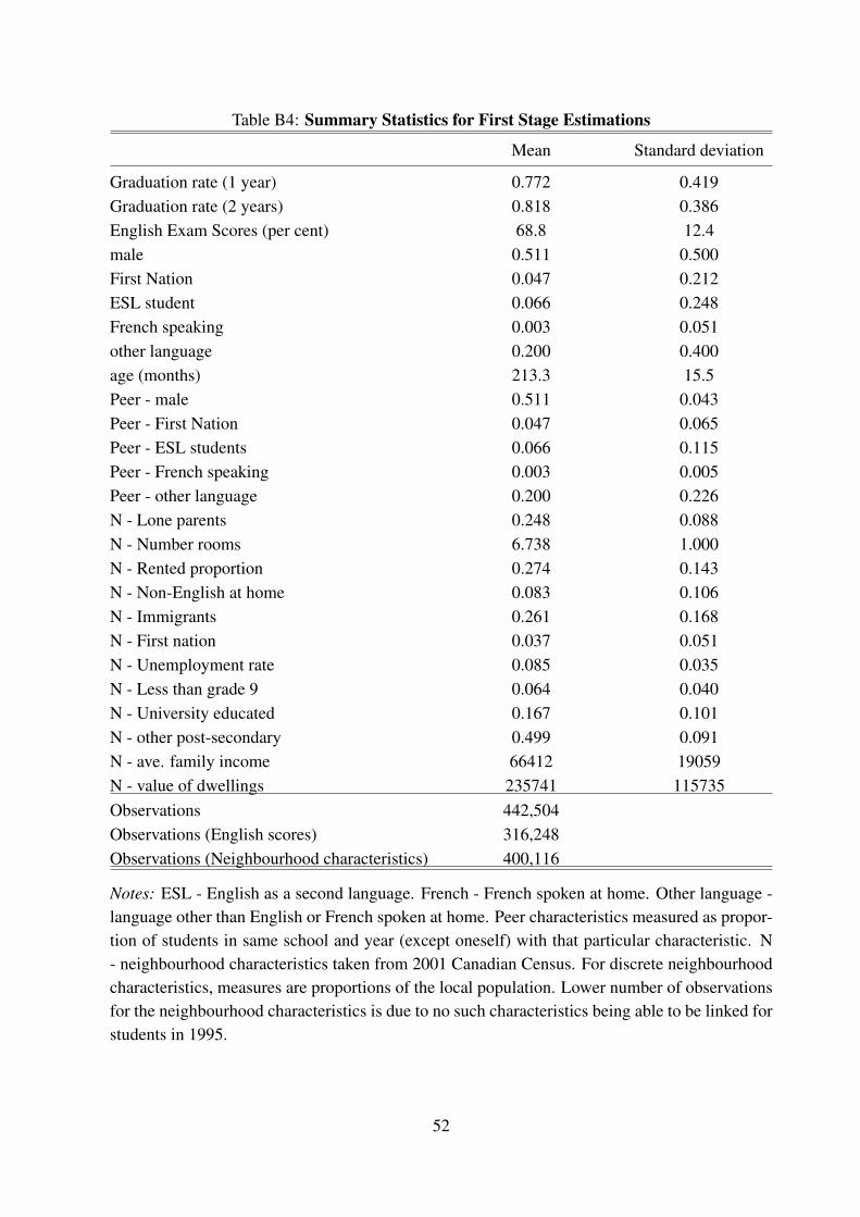
Table B4: Summary Statistics for First Stage Estimations

Mean Standard deviation

Graduation rate (1 year) 0.772 0.419Graduation rate (2 years) 0.818 0.386English Exam Scores (per cent) 68.8 12.4male 0.511 0.500First Nation 0.047 0.212ESL student 0.066 0.248French speaking 0.003 0.051other language 0.200 0.400age (months) 213.3 15.5Peer - male 0.511 0.043Peer - First Nation 0.047 0.065Peer - ESL students 0.066 0.115Peer - French speaking 0.003 0.005Peer - other language 0.200 0.226N - Lone parents 0.248 0.088N - Number rooms 6.738 1.000N - Rented proportion 0.274 0.143N - Non-English at home 0.083 0.106N - Immigrants 0.261 0.168N - First nation 0.037 0.051N - Unemployment rate 0.085 0.035N - Less than grade 9 0.064 0.040N - University educated 0.167 0.101N - other post-secondary 0.499 0.091N - ave. family income 66412 19059N - value of dwellings 235741 115735Observations 442,504Observations (English scores) 316,248Observations (Neighbourhood characteristics) 400,116

Notes: ESL - English as a second language. French - French spoken at home. Other language -language other than English or French spoken at home. Peer characteristics measured as propor-tion of students in same school and year (except oneself) with that particular characteristic. N- neighbourhood characteristics taken from 2001 Canadian Census. For discrete neighbourhoodcharacteristics, measures are proportions of the local population. Lower number of observationsfor the neighbourhood characteristics is due to no such characteristics being able to be linked forstudents in 1995.

52

ReferencesAaronson, D., Barrow, L., & Sander, W. (2007). Teachers and Student Achievement in the

Chicago Public High Schools. Journal of Labor Economics, 25 (1), 95-135, January.Aman, Cheryl (2010). The Relationship of Student Mobility to Graduation Rates in Three

Kindergarten to Grade 12 Cohorts in British Columbia. Canadian Council on LearningCommissioned Report, Ottawa, Ontario.

Armor, D., Conry-Osequera, P., Cox, M., King, N., McDonnell, L., Pascal, A., Pauly, E. &Zellman, G. (1976). Analysis of the school preferred reading program in selected LosAngeles minority schools. R-2007-LAUSD, Rand Corporation, Santa Monica.

Beresford, C., & Heather Fussell (2009). When More is Less: Education Funding in BC. Centrefor Civic Governance.

Boudarbat, Brahim, Thomas Lemieux, and W. Craig Riddell (2010). The Evolution of the Re-turns to Human Capital in Canada. Canadian Public Policy, 36 (1), 63-89.

Bowlby, Geoff (2005). Provincial Drop-out Rates - Trends and Consequences. Education Mat-ters, Vol. 2, No. 4.

Branch, Gregory F., Eric A. Hanushek & Steven G. Rivkin (2008). Principal Turnover and Effec-tiveness. Paper prepared for the annual meetings of the American Economics Association,San Francisco, CA.

British Columbia Ministry of Education (2008). Policy Document: K-12 Funding - General.Issued September 1, 2002. Revised, July 1, 2008.

Brock, William A. & Steven N. Durlauf (2001). Interactions-Based Models. In J.J. Heckman &E. Leamer, Handbook of Econometrics, Volume 5 (pp. 3297-3380). North-Holland.

Carneiro, Pedro, K. T. Hansen, & James J. Heckman (2003). Estimating Distributions of Treat-ment Effects with an Application to the Returns to Schooling and Measurement of theEffects of Uncertainty on College Choice. International Economic Review, 44 (2), 361-422.

Clark, Damon, Paco Martorell & Jonah Rockoff (2009). School Principals and School Per-formance. Center for Analysis of Longitudinal Data in Education Research (CALDER)Working Paper no. 38, Urban Institute.

Coleman, James S., Ernest Q. Campbell, Carol J. Hobson, James McPartland, Alexander M.Mood, Frederic D. Weinfeld, & Robert L. York (1966) Equality of educational opportunity.Washington DC: U.S. Government Printing Office.

Cullen, Julie B. & Michael J. Mazzeo (2007). Implicit Performance Awards: An EmpiricalAnalysis of the Labor Market for Public School Administrators. Unpublished manuscript,UC San Diego and Northwestern.

Figlio, David (2006). Testing, Crime and Punishment. Journal of Public Economics, 90 (4-5),837-851.

Foley, Kelly (2010). Can Neighbourhoods Change the Decisions of Youth on the Margins ofUniversity Participation? Copenhagen Business School Working Paper.

Friesen, Jane & Brian Krauth (forthcoming). Sorting, Peers and Achievement of AboriginalStudents in British Columbia. Canadian Journal of Economics.

53

Gates, Susan M., Jeanne S. Ringel, Lucrecia Santibaez, Cassandra Guarino, Bonnie Ghosh-Dastidar, & Abigail Brown (2006). Mobility and turnover among school principals. Eco-nomics of Education Review, 25 (3), 289-302.

Gilmore, Jason (2010). Trends in Dropout Rates and the Labour Market Outcomes of YoungDropouts. Education Matters, Statistics Canada, 7 (4).

Goldhaber, Dan D., & Dominic J. Brewer (1997). Why Don’t Schools and Teachers Seem toMatter? Assessing the Impact of Unobservables on Educational Productivity. The Journalof Human Resources, 32 (3), 505-523.

Hallinger, Philip & Ronald H. Heck (1998). Exploring the Principal’s Contribution to SchoolEffectiveness: 1980-1995. School Effectiveness and School Improvement, 9 (2), 157-191.

Hanushek, Eric A. (1971). Teacher Characteristics and Gains in Student Achievement: Estima-tion Using Micro Data. The American Economic Review: Papers and Proceedings, 61 (2),280-288.

Hanushek, Eric A. (2003). The failure of input-based schooling policies. The Economic Journal,113, F64-F98.

Jacob, Brian A. & Steven D. Levitt (2003). Rotten Apples: An Investigation of the Prevalenceand Predictors of Teacher Cheating. Quarterly Journal of Economics, 118 (3), 843-77.

Kane, Thomas J., Jonah E. Rockoff & Douglas O. Staiger (2008). What Does Certification TellUs About Teacher Effectiveness? Economics of Education Review, 27 (6), 615-631.

Koedel, Cory (2008). Teacher quality and dropout outcomes in a large, urban school district.Journal of Urban Economics, 64 (3), 560-572.

Konstantopoulos, Spyros (2007). How Long Do Teacher Effects Persist? Institute for the Studyof Labor (IZA) Discussion Paper No. 2893, Bonn.

Krueger, Alan (2003). Economic considerations and class size. The Economic Journal, 113,F34-F63.

Lavy, Victor (2008). Does Raising the Principals Wage Improve the Schools Outcomes? Quasi-experimental Evidence from an Unusual Policy Experiment in Israel. Scandinavian Jour-nal of Economics, 110 (4), 639662.

Leigh, Andrew (2007). Estimating Teacher Effectiveness from Two-Year Changes in Students’Test Scores. Unpublished manuscript, Australian National University, May.

Leithwood, Kenneth & Doris Jantzi (1999). The Relative Effects of Principal and TeacherSources of Leadership on Student Engagement with School. Education AdministrationQuarterly, 35 (Supplemental), 679-706.

Manski, Charles F. (1993). Identification of Endogenous Social Effects: The Reflection Problem.The Review of Economic Studies, 60 (3), 531-542.

McNeil, Linda McSpadden, Eileen Coppola, Judy Radigan, & Julian Vasquez Heilig (2008).Avoidable Losses: High Stakes Accountability and the Dropout Crisis. Education PolicyAnalysis Archives, 16 (3), 1-48.

Miller, Ashley (2009). Principal Turnover, Student Achievement and Teacher Retention. unpub-lished manuscript, Princeton University.

54

Murnane, Richard J., & Barbara R. Phillips (1981). What do effective teachers of inner-citychildren have in common? Social Science Research, 10 (1), 83-100.

Nye, Barbara, Spyros Konstantopoulos & Larry V. Hedges (2004). How Large are TeacherEffects? Educational Evaluation and Policy Analysis, 26 (3), 237-257.

Park, Albert & Emily Hannum (2002). Do Teachers Affect Learning in Developing Countries?Evidence from Matched StudentTeacher Data from China. Unpublished manuscript, Uni-versity of Michigan, April.

Rivkin, Steven G., Eric A. Hanushek & John F. Kain (2005). Teachers, Schools and AcademicAchievement. Econometrica, 73 (2), 417-458.

Rockoff, Jonah E. (2004). The Impact of Individual Teachers on Student Achievement: Evidencefrom Panel Data. American Economic Review: Papers and Proceedings, 96 (2), 247-252.

Rowan, Brian, Richard Correnti & Robert J. Miller (2002). What large scale, survey researchtells us about teacher effects on student achievement: Insights from the Prospects study ofelementary schools. Teachers College Record, 104 (8), 1525-1567.

Todd, Petra E. & Kenneth I. Wolpin (2003). On the Specification and Estimation of the Produc-tion Function for Cognitive Achievement. The Economic Journal, 113, F3-F33.

Uribe, Claudia, Richard J. Murnane & John B Willett (2003). Why Do Students Learn Morein Some Classrooms Than in Others? Evidence from Bogota. Working paper, HarvardGraduate School of Education, November.

55