Lattice calibration with turn-by-turn BPM...
17
3/17/2010 1 Lattice calibration with turn-by-turn BPM data X. Huang 3/17/2010 IUCF Workshop -- X. Huang
Transcript of Lattice calibration with turn-by-turn BPM...

3/17/2010 1
Lattice calibration with turn-by-turn BPM data
X. Huang3/17/2010
IUCF Workshop -- X. Huang
Outline• Lattice calibration methods
– Orbit response matrix – LOCO– Turn-by-turn BPM data – MIA, ICA, etc.
• Transfer matrix from turn-by-turn BPM data• Model fitting with turn-by-turn data
– Simple case– General case– Simulation results
3/17/2010 IUCF Workshop -- X. Huang 2
Benefits of lattice calibration• Lattice calibration: set machine optics/nonlinearity to the
ideal case (model) – usually symmetric and periodic.• Benefit of lattice calibration
– Reliable model for ring parameter evaluations– Reduce resonance driving terms.– Reduce maximum beta function and dispersion.– Discover human errors – wrong cabling, wrong setpoint, etc
3/17/2010 IUCF Workshop -- X. Huang 3
Calibrated rings tend to have increased injection efficiency, lifetime and stability.
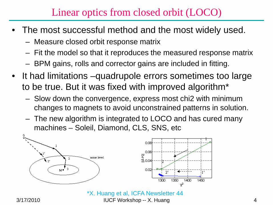
Linear optics from closed orbit (LOCO)• The most successful method and the most widely used.
– Measure closed orbit response matrix– Fit the model so that it reproduces the measured response matrix– BPM gains, rolls and corrector gains are included in fitting.
• It had limitations –quadrupole errors sometimes too large to be true. But it was fixed with improved algorithm*– Slow down the convergence, express most chi2 with minimum
changes to magnets to avoid unconstrained patterns in solution.– The new algorithm is integrated to LOCO and has cured many
machines – Soleil, Diamond, CLS, SNS, etc
3/17/2010 IUCF Workshop -- X. Huang 4*X. Huang et al, ICFA Newsletter 44

Methods based on turn-by-turn BPM data• Analyze simultaneous turn-by-turn BPM data
– MIA, principal component analysis or SVD– ICA, independent component analysis– Other methods (Sussix?, harmonic analysis?, and more)
• Can obtain precise phase advance measurements, but beta functions are coupled with BPM gains.
• Fit the model for phase advance, beta and dispersion.• Fitting beta functions and phase advances is not the most
convenient– Cannot include BPM gains in fitting– Loss of information in case of coupled motion and nonlinear motion.
3/17/2010 IUCF Workshop -- X. Huang 5
Calibration of nonlinearity• Nonlinear LOCO
– Orbit response with large corrector kicks
• Fitting nonlinear resonance driving terms obtained from turn-by-turn BPMs (R. Bartolini)
• ICA for sextupoles (X. Pang)– Identify an independent mode driven by sextupoles.
3/17/2010 IUCF Workshop -- X. Huang 6

A new method for lattice calibration• Derive 4D phase space coordinates from two BPMs.• Fit turn-by-turn orbit data directly by comparing
measurements to tracking.
3/17/2010 IUCF Workshop -- X. Huang 7
Suppose BPM 1, 2 are separated by a drift space with length L.
Fit for the transfer matrix
3/17/2010 IUCF Workshop -- X. Huang 8
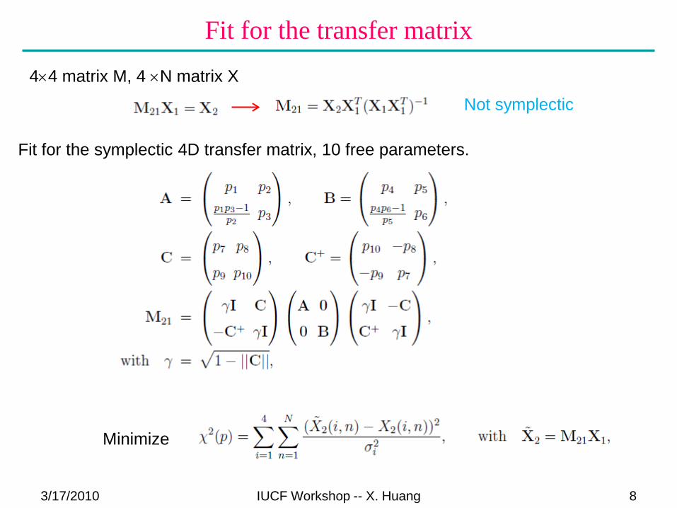
4×4 matrix M, 4 ×N matrix X
Not symplectic
Fit for the symplectic 4D transfer matrix, 10 free parameters.
Minimize

A simulated case
3/17/2010 IUCF Workshop -- X. Huang 9
Fitted matrix
Matrix calculated from model
Differences between fitted and calculated matrices are from BPM noises and lattice nonlinearities.
Tracking data with 50 µm noise
Normal mode coordinates obtained with fitted matrix
Calibration of one quadrupole
3/17/2010 IUCF Workshop -- X. Huang 10
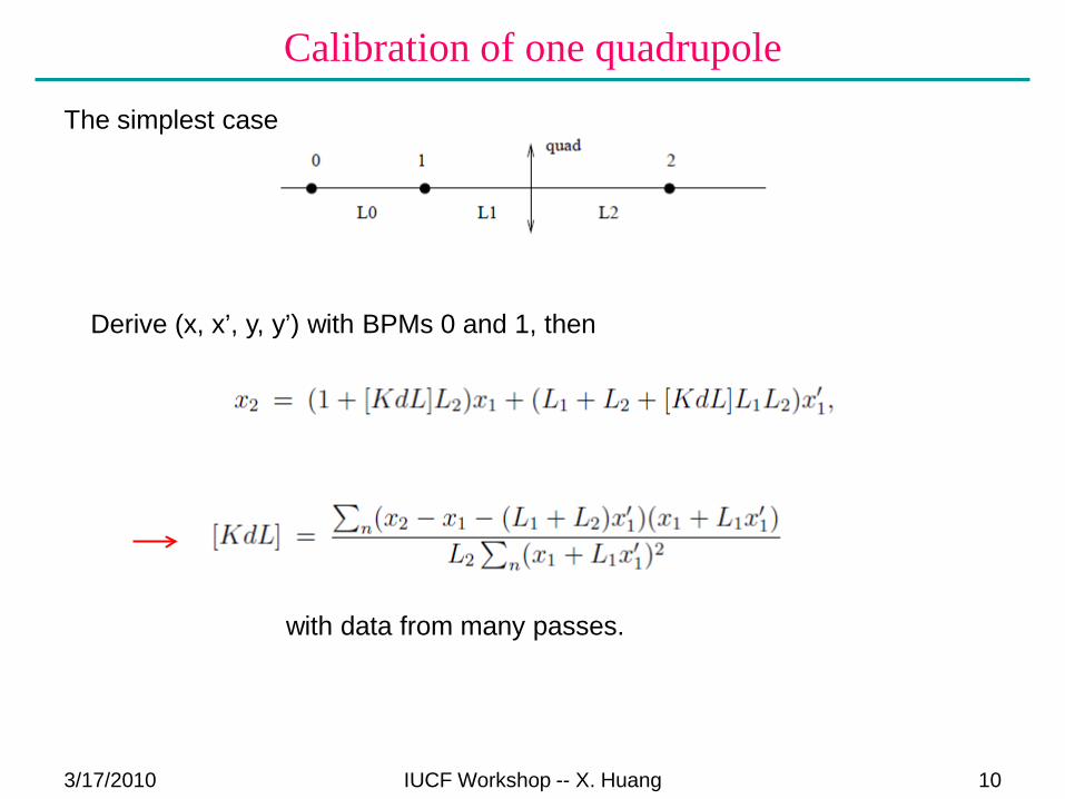
The simplest case
Derive (x, x’, y, y’) with BPMs 0 and 1, then
with data from many passes.

A general accelerator section
3/17/2010 IUCF Workshop -- X. Huang 11
Do not consider gains and rolls for BPM 0, 1Consider gains and rolls for other BPMs:
BPM readingActual coordinates
Fit turn-by-turn data BPM reading Predictions from tracking
Use the usual iterative least-square fitter:
Jacobian matrixDefine residual vector r
Solve for
Simulation with SPEAR3 model
3/17/2010 IUCF Workshop -- X. Huang 12
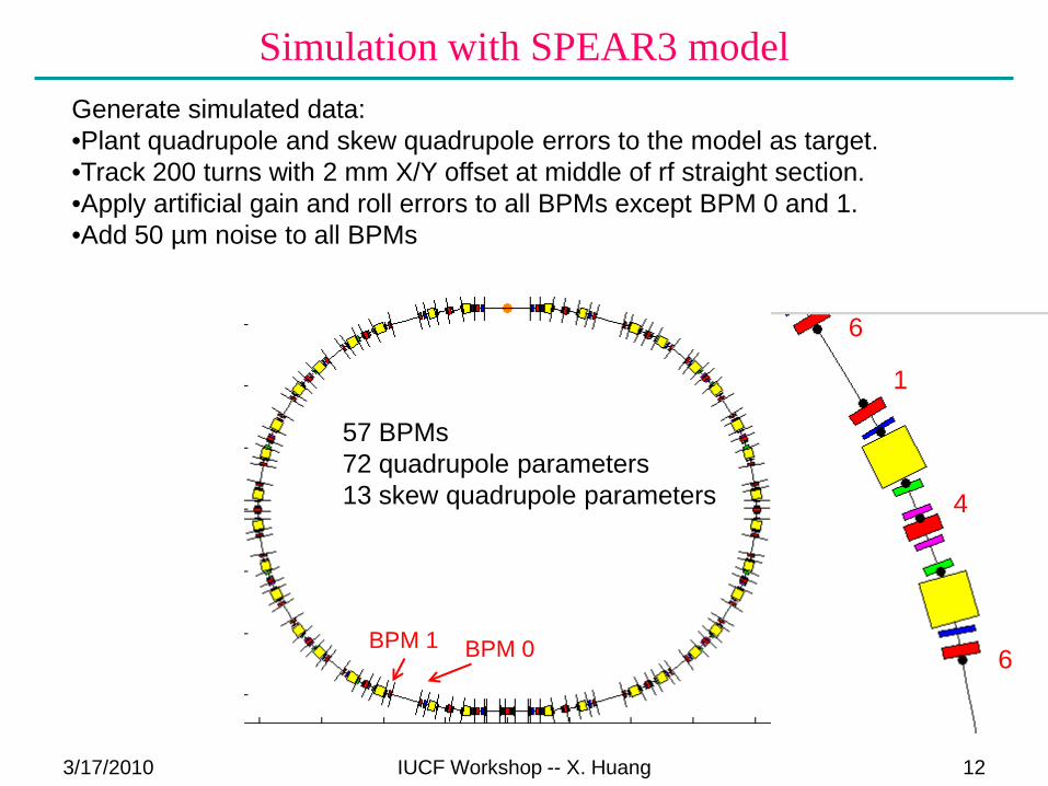
BPM 0BPM 1
57 BPMs72 quadrupole parameters13 skew quadrupole parameters
Generate simulated data:•Plant quadrupole and skew quadrupole errors to the model as target.•Track 200 turns with 2 mm X/Y offset at middle of rf straight section.•Apply artificial gain and roll errors to all BPMs except BPM 0 and 1.•Add 50 µm noise to all BPMs
1
4
6
6
Quadrupole results
3/17/2010 IUCF Workshop -- X. Huang 13
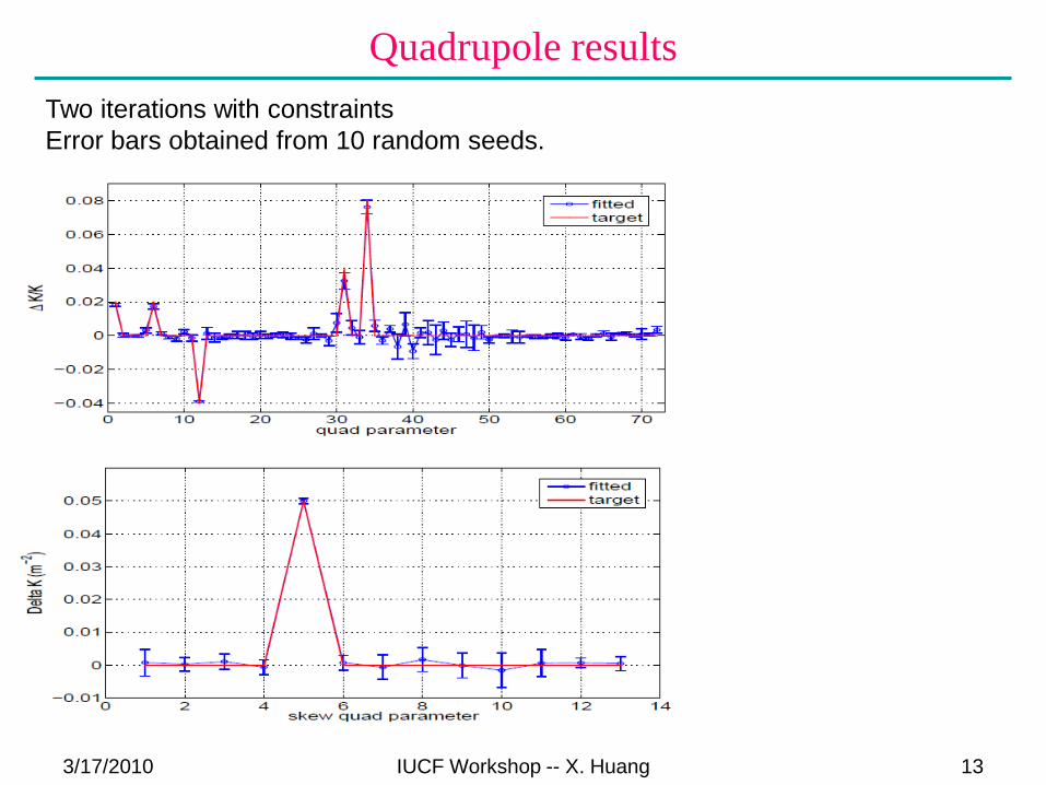
Two iterations with constraintsError bars obtained from 10 random seeds.

BPM parameters
3/17/2010 IUCF Workshop -- X. Huang 14
Including sextupoles
3/17/2010 IUCF Workshop -- X. Huang 15
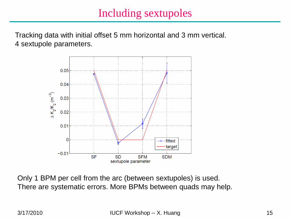
Tracking data with initial offset 5 mm horizontal and 3 mm vertical.4 sextupole parameters.
Only 1 BPM per cell from the arc (between sextupoles) is used. There are systematic errors. More BPMs between quads may help.
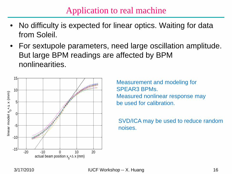
Application to real machine• No difficulty is expected for linear optics. Waiting for data
from Soleil.• For sextupole parameters, need large oscillation amplitude.
But large BPM readings are affected by BPM nonlinearities.
3/17/2010 IUCF Workshop -- X. Huang 16
-20 -10 0 10 20-15
-10
-5
0
5
10
15
actual beam position x0+∆ x (mm)
linear
model x
0+∆
x (
mm
)
Measurement and modeling for SPEAR3 BPMs.Measured nonlinear response may be used for calibration.
SVD/ICA may be used to reduce random noises.

Summary• The new method fit turn-by-turn BPM directly to model.• Advantages:
– Fast data acquisition. – Can fit BPM gains and rolls.– Natural choice for beam motion with linear coupling and nonlinear
response.
• Disadvantages:– Gain and roll errors, noises in BPM 0 and 1 propagate to tracking
data.
3/17/2010 IUCF Workshop -- X. Huang 17