CAI, LIU, YU, SHAO: LATENT STRUCTURE PRESERVING HASHING 1

Latent Structure Preserving Hashing

Ziyun Cai1

cziyun1@sheffield.ac.uk

Li Liu2

li2.liu@northumbria.ac.uk

Mengyang Yu2

m.y.yu@ieee.org

Ling Shao2

ling.shao@ieee.org

1 Department of Electronic and ElectricalEngineeringThe University of SheffieldSheffield, S1 3JD, UK

2 Computer Vision and ArtificialIntelligence GroupDepartment of Computer Science andDigital TechnologiesNorthumbria UniversityNewcastle upon Tyne, NE1 8ST, UK

Abstract

Aiming at efficient similarity search, hash functions are designed to embed high-dimensional feature descriptors to low-dimensional binary codes such that similar de-scriptors will lead to the binary codes with a short distance in the Hamming space. It iscritical to effectively maintain the intrinsic structure and preserve the original informa-tion of data in a hashing algorithm. In this paper, we propose a novel hashing algorithmcalled Latent Structure Preserving Hashing (LSPH), with the target of finding a well-structured low-dimensional data representation from the original high-dimensional datathrough a novel objective function based on Nonnegative Matrix Factorization (NMF).Via exploiting the probabilistic distribution of data, LSPH can automatically learn the la-tent information and successfully preserve the structure of high-dimensional data. Afterfinding the low-dimensional representations, the hash functions can be acquired throughmulti-variable logistic regression. Experimental results on two large-scale datasets, i.e.,SIFT 1M and GIST 1M, show that LSPH can significantly outperform the state-of-the-art hashing techniques.

1 IntroductionSimilarity search [3, 11, 19, 22] is one of the most critical problems in information retrievalas well as in pattern recognition, data mining and machine learning. Generally speaking,effective similarity search approaches try to construct the index structure in the metric space.However, with the increase of the dimensionality of the data, how to implement the similar-ity search efficiently and effectively has become an significant topic. To improve retrievalefficiency, hashing algorithms are deployed to find a hash function from Euclidean space toHamming space. The hashing algorithms with binary coding techniques mainly have twoadvantages: (1) binary hash codes save storage space; (2) it is efficient to compute the Ham-ming distance (XOR operation) between the training data and the new coming data in theretrieval procedure of similarity search. The time complexity of searching the hashing tableis near O(1).

c© 2015. The copyright of this document resides with its authors.It may be distributed unchanged freely in print or electronic forms. Pages 172.1-172.11

DOI: https://dx.doi.org/10.5244/C.29.172

2 CAI, LIU, YU, SHAO: LATENT STRUCTURE PRESERVING HASHING

NMF

Database

1

0

Hash functiongeneration

Data distribution

Part-based

latent in

form

ation

0101

1010

1100

0011

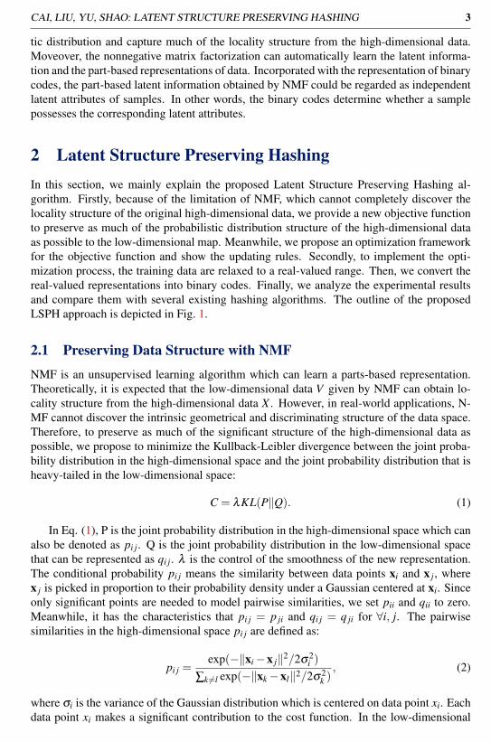
Figure 1: The outline of the proposed method. Part-based latent information is learned fromNMF with the regularization of data distribution.

Current hashing algorithms can be roughly divided into random projection based orlearning based. Locality Sensitive Hashing (LSH) [3] is one of the most widely used hash-ing algorithms based on random linear projections, which can efficiently map the data pointsfrom the high-dimensional space into the low-dimensional Hamming space. Kernelized Lo-cality Sensitive Hashing (KLSH) [7] can exploit more significant similarity in kernel spacefor better retrieval effectiveness. However, the random projection based hash functions areeffective only when the binary hash code is long enough. Through mining the structure ofthe data, then being represented on the objective function, a learning based hashing algo-rithm can obtain the hash function by solving an optimization problem associated with theobjective function. Spectral Hashing (SpH) [20] is a representative unsupervised hashingmethod, which can learn compact binary codes that preserve the similarity between docu-ments by forcing the balanced and uncorrelated constraints into the learned codes. In [18],Principal Component Analysis Hashing (PCAH) has been introduced for better quantizationrather than random projection hashing. Moreover, Semantic Hashing (SH), which is basedon Restricted Boltzmann Machines (RBM) [16], was proposed in [15]. Liu et al. [12] pro-posed an Anchor Graph-based Hashing method (AGH), which automatically discovers theneighborhood structure inherent in the data to learn appropriate compact codes. More re-cently, Spherical Hashing (SpherH) [5] and Iterative Quantization (ITQ) [4] were developedfor more compact and effective binary coding. Additionally, Boosted Similarity SensitiveCoding (BSSC) [17], Compressed Hashing (CH) [10] and Self-taught Hashing (STH) [22]are also successfully utilized for large-scale visual retrieval tasks.

However, the above mentioned hashing methods have their limitations. Though the ran-dom projection based hashing methods can produce compact codes, the simple, linear hashfunctions cannot reflect the underlying relationship between the data points. Meanwhile,since the linear formulation is computed with a high-dimensional matrix, it will result in aheavy computational cost. On the other hand, the learning based hashing algorithms are notefficient when the codewords are long. Besides, those hashing approaches, which first reducethe dimensionality of the original data, cannot obtain a well-structured low-dimensional datarepresentation.

In order to overcome these limitations, we propose a novel NMF-based approach calledLatent Structure Preserving Hashing (LSPH) which can effectively preserve data probabilis-

CAI, LIU, YU, SHAO: LATENT STRUCTURE PRESERVING HASHING 3

tic distribution and capture much of the locality structure from the high-dimensional data.Moveover, the nonnegative matrix factorization can automatically learn the latent informa-tion and the part-based representations of data. Incorporated with the representation of binarycodes, the part-based latent information obtained by NMF could be regarded as independentlatent attributes of samples. In other words, the binary codes determine whether a samplepossesses the corresponding latent attributes.

2 Latent Structure Preserving HashingIn this section, we mainly explain the proposed Latent Structure Preserving Hashing al-gorithm. Firstly, because of the limitation of NMF, which cannot completely discover thelocality structure of the original high-dimensional data, we provide a new objective functionto preserve as much of the probabilistic distribution structure of the high-dimensional dataas possible to the low-dimensional map. Meanwhile, we propose an optimization frameworkfor the objective function and show the updating rules. Secondly, to implement the opti-mization process, the training data are relaxed to a real-valued range. Then, we convert thereal-valued representations into binary codes. Finally, we analyze the experimental resultsand compare them with several existing hashing algorithms. The outline of the proposedLSPH approach is depicted in Fig. 1.

2.1 Preserving Data Structure with NMF

NMF is an unsupervised learning algorithm which can learn a parts-based representation.Theoretically, it is expected that the low-dimensional data V given by NMF can obtain lo-cality structure from the high-dimensional data X . However, in real-world applications, N-MF cannot discover the intrinsic geometrical and discriminating structure of the data space.Therefore, to preserve as much of the significant structure of the high-dimensional data aspossible, we propose to minimize the Kullback-Leibler divergence between the joint proba-bility distribution in the high-dimensional space and the joint probability distribution that isheavy-tailed in the low-dimensional space:

C = λKL(P‖Q). (1)

In Eq. (1), P is the joint probability distribution in the high-dimensional space which canalso be denoted as pi j. Q is the joint probability distribution in the low-dimensional spacethat can be represented as qi j. λ is the control of the smoothness of the new representation.The conditional probability pi j means the similarity between data points xi and x j, wherex j is picked in proportion to their probability density under a Gaussian centered at xi. Sinceonly significant points are needed to model pairwise similarities, we set pii and qii to zero.Meanwhile, it has the characteristics that pi j = p ji and qi j = q ji for ∀i, j. The pairwisesimilarities in the high-dimensional space pi j are defined as:

pi j =exp(−‖xi−x j‖2/2σ2

i )

∑k 6=l exp(−‖xk−xl‖2/2σ2k )

, (2)

where σi is the variance of the Gaussian distribution which is centered on data point xi. Eachdata point xi makes a significant contribution to the cost function. In the low-dimensional

4 CAI, LIU, YU, SHAO: LATENT STRUCTURE PRESERVING HASHING

map, using the probability distribution that is heavy tailed, the joint probabilities qi j can bedefined as:

qi j =(1+‖vi−v j‖2)−1

∑k 6=l(1+‖vk−vl‖2)−1 . (3)

This definition is an infinite mixture of Gaussians, which is much faster to evaluate the den-sity of a point than the single Gaussian, since it does not have an exponential. This represen-tation also makes the mapped points invariant to the changes in the scale for the embeddedpoints that are far apart. Thus, the cost function based on Kullback-Leibler divergence caneffectively measure the significance of the data distribution . qi j models pi j is given by

G = KL(P‖Q) = ∑i

∑j

pi j log pi j− pi j logqi j. (4)

For simplicity, we define two auxiliary variables di j and Z for making the derivation cleareras follows:

di j = ‖vi−v j‖ and Z = ∑k 6=l

(1+d2kl)−1. (5)

Therefore, the gradient of function G with respect to vi can be given by

∂G∂vi

= 2N

∑j=1

∂G∂di j

(vi−v j). (6)

Then ∂G∂di j

can be calculated by Kullback-Leibler divergence in Eq. (4):

∂G∂di j

=−∑k 6=l

pkl

(1

qklZ∂ ((1+d2

kl)−1)

∂di j− 1

Z∂Z∂di j

). (7)

Since ∂ ((1+d2kl)−1)

∂di jis nonzero if and only if k = i and l = j, and ∑k 6=l pkl = 1, the gradient

function can be expressed as

∂G∂di j

= 2(pi j−qi j)(1+d2i j)−1. (8)

Eq. (8) can be substituted into Eq. (6). Therefore, the gradient of the Kullback-Leiblerdivergence between P and Q is

∂G∂vi

= 4N

∑j=1

(pi j−qi j)(vi−v j)(1+‖vi−v j‖2)−1. (9)

Therefore, through combining the data structure preserving part in Eq. (1) and the NMFtechnique, we can obtain the following new objective function:

O f = ‖X−UV‖2 +λKL(P‖Q), (10)

where V ∈ {0,1}D×N , X ,U,V > 0, U ∈ RM×D, X ∈ RM×N , and λ controls the smoothnessof the new representation.

In most of the circumstances, the low-dimensional data only from NMF is not effectiveand meaningful for realistic applications. Thus, we introduce λKL(P‖Q) to preserve thestructure of the original data which can obtain better results in information retrieval.

CAI, LIU, YU, SHAO: LATENT STRUCTURE PRESERVING HASHING 5

2.2 Relaxation and OptimizationSince the discreteness condition V ∈ {0,1}D×N in Eq. (10) cannot be calculated directly inthe optimization procedure, motivated by [20], we first relax the data V ∈ {0,1}D×N to therange V ∈ RD×N for obtaining real-values. Then let the Lagrangian of our problem be:

L= ‖X−UV‖2 +λKL(P‖Q)+ tr(ΦUT )+ tr(ΨV T ), (11)

where matrices Φ and Ψ are two Lagrangian multiplier matrices. Since we have the gradientof C = λG:

∂C∂vi

= 4λ

N

∑j=1

(pi j−qi j)(vi−v j)(1+‖vi−v j‖2)−1, (12)

we make the gradients of L be zeros to minimize O f :

∂L∂V

= 2(−UT X +UTUV )+∂C∂vi

+Ψ = 0, (13)

∂L∂U

= 2(−XV T +UVV T )+Φ = 0, (14)

In addition, we also have KKT conditions: Φi jUi j = 0 and Ψi jVi j = 0, ∀i, j. Then multiplyingVi j and Ui j in the corresponding positions on both sides of Eqs. (13) and (14) respectively,we obtain

(2(−UT X +UTUV )+∂C∂vi

)i jVi j = 0, (15)

2(−XV T +UVV T )i jUi j = 0. (16)

Note that (∂C∂v j

)i=

(4λ

N

∑k=1

p jkv j−q jkv j− p jkvk +q jkvk

1+‖v j−vk‖2

)i

= 4λ

N

∑k=1

p jkVi j−q jkVi j− p jkVik +q jkVik

1+‖v j−vk‖2 .

Therefore, we have the following update rules for any i, j:

Vi j ←(UT X)i j +2λ

N∑

k=1

p jkVik+q jkVi j1+‖v j−vk‖2

(UTUV )i j +2λN∑

k=1

p jkVi j+q jkVik1+‖v j−vk‖2

Vi j, (17)

Ui j ←(XV T )i j

(UVV T )i jUi j. (18)

All the elements in U and V can be guaranteed that they are nonnegative from the allo-cation. In [8], it has been proved that the objective function is monotonically non-increasingafter each update of U or V . The proof of convergence about U and V is similar to the onesin [2, 23].

6 CAI, LIU, YU, SHAO: LATENT STRUCTURE PRESERVING HASHING

2.3 Hash Function GenerationThe low-dimensional representations V ∈ RD×N and the bases U ∈ RM×D, where D� M,can be obtained from Eq. (17) and Eq. (18), respectively. Then we need to convert the low-dimensional real-valued representations from V = [v1, · · · ,vN ] into binary codes via thresh-olding: if the d-th element in vn is larger than a specified threshold, this real value will berepresented as 1; otherwise it will be 0, where d = 1, · · · ,D and n = 1, · · · ,N.

In addition, a well-designed semantic hashing should also be entropy maximizing toensure its efficiency [1]. Meanwhile, from the information theory, through having a uniformprobability distribution, the source alphabet can reach a maximal entropy. Specifically, if theentropy of codes over the corpus is small, the documents will be mapped to a small numberof codes (hash bins). In this paper, the threshold of the elements in vn can be set to the medianvalue of vn, which can satisfy entropy maximization. Therefore, half of the bit-strings willbe 1 and the other half will be 0. In this way, the real-value code can be calculated into abinary code [21].

However, from the above procedure, we can only obtain the binary codes of the data inthe training set. Therefore, given a new sample, it cannot directly find a hash function. In ourapproach, due to the binary code environment, we use the logistic regression [6] which can betreated as a type of probabilistic statistical classification model to compute the hash code inthe test set. Before obtaining the logistic regression cost function, we define that the binarycode is represented as V̂ = [v̂1, · · · , v̂N ], where v̂n ∈ {0,1}D and n = 1, · · · ,N. Therefore,the training set can be considered as {(v1, v̂1),(v2, v̂2), · · · ,(vN , v̂N)}. The vector-valuedregression function which is based on the corresponding regression matrix Θ ∈RD×D can berepresented as

hΘ(vn) =

(1

1+ e−(ΘT vn)i

)T

i=1,··· ,D. (19)

Therefore, with the maximum log-likelihood criterion for the Bernoulli-distributed data, ourcost function for the corresponding regression matrix can be defined as:

J(Θ) =− 1N

(N

∑n=1

(v̂T

n log(hΘ(vn))+(1− v̂n)T log(1−hΘ(vn))

)+δ‖Θ‖2

), (20)

where log(·) is the element-wise logarithm function and 1 is an D× 1 all ones matrix. Weuse δ‖Θ‖2 as the regularization term in logistic regression to avoid overfitting.

To find the matrix Θ which aims to minimize J(Θ), we use gradient descent and re-peatedly update each parameter using a learning rate α . The updating equation is shown asfollows:

Θ(t+1) = Θ

(t)− α

N

N

∑n=1

(hΘ(t)(vn)− v̂n)vT

n −αδ

NΘ

(t). (21)

The updating equation stops when the norm of difference between Θ(t+1) and Θ(t), i.e.,||Θ(t+1)−Θ(t)||2, is smaller than a small value. Then we can obtain the regression matrix Θ.

After this, we can obtain the real-valued low-dimensional representation through a linearprojection matrix Q = (UTU)−1UT , which is the pseudoinverse of U . Since we have X ≈UV , applying the projection matrix Q to the data matrix X , we obtain QX = (UTU)−1UT X ≈(UTU)−1UTUV =V . Note that each entry of hΘ is a sigmoid function, the hash codes for anew coming sample Xnew ∈ RM×1 can be represented as:

V̂new = bhΘ(QXnew)e, (22)

CAI, LIU, YU, SHAO: LATENT STRUCTURE PRESERVING HASHING 7

where b·e means the nearest integer function for each entry of hΘ. We define that the thresh-old of binarization is 0.5. Therefore, if a bit from hΘ(QXnew) is larger than 0.5, it will berepresented as 1, otherwise 0. For example, through Eq. (22), vector [0.17, 0.37, 0.50, 0.79,0.03, 0.92, · · · ] is expressed as [0, 0, 0, 1, 0, 1, · · · ]. Up to now, we can obtain the LatentStructure Preserving Hashing codes for both training and test data. The procedure of LSPHis summarized in Algorithm 1.

Algorithm 1 Latent Structure Preserving Hashing (LSPH)Input:

The training matrix X ∈RM×N ; the objective dimension (code length) D of hash codes; the learningrate α for logistic regression; the regularization parameters {δ , λ}.

Output:The basis matrix U and the regression matrix Θ.

1: repeat2: Compute the low-dimensional representation matrix V and the basis matrix U via Eq. (17) and Eq.

(18);3: until convergence4: Obtain the regression matrix Θ through Eq. (21) and the final LSPH encoding for each sample is

defined in Eq. (22).

2.4 Computational Complexity AnalysisIn this section, we will discuss the computational complexity of our LSPH, which consists ofthree parts. The first part is for computing NMF, the complexity of which is O(NMKD) [9],where N is the size of the dataset, M and D are the dimensionalities of the high-dimensionaldata and the low-dimensional data respectively and K is the number of classes in this dataset.The second part is to compute the cost function Eq. (4) in the objective function which hasthe complexity O(N2D). The last part is the logistic regression procedure whose complexityis O(ND2). Therefore, the total computational complexity of LSPH is: O(tNMKD+N2D+tND2), where t is the number of iterations.

3 ExperimentsTo evaluate our unsupervised LSPH algorithm on the similarity search problem, we performexperiments on two large-scale datasets: SIFT 1M with local SIFT descriptors [13] andGIST 1M with global GIST descriptors [14]. The SIFT 1M dataset has one million datapoints, the dimensionality of which is 128. The GIST 1M dataset has the same number ofdata points, but the dimensionality is 960. All the experiments are performed using Matlab2013a on a server configured with a 12-core processor and 128GB RAM running the LinuxOS.

In our experiments, 10K data points are selected as the queries at random. At the sametime, the rest of the dataset can be considered as the image database. During the test phase, ifthe returned point is in the top 2 percentile points closest to a query, it will be considered asa true neighbor. Since the Hamming distance ranking is fast with hash codes, we will use theHamming distance ranking to measure our retrieval tasks. The experimental results can bemeasured by the Mean Average Precision (MAP) and precision-recall curves. Meanwhile,we will also compare the training time and the test time in all the selected algorithms.

8 CAI, LIU, YU, SHAO: LATENT STRUCTURE PRESERVING HASHING

Figure 2: The Mean Average Precision of the compared algorithms on the SIFT 1M andGIST 1M datasets.

3.1 The Selected Methods and Setting

In this part, we compare LSPH with the 10 selected popular hashing methods including LSH[3], BSSC [17], RBM [16], SpH [20], STH [22], AGH [12], ITQ [4], KLSH [7], PCAH[18] and CH [10]. In these methods, for BSSC, through the labeled pairs scheme in theboosting framework, it can obtain weights and thresholds for every hash function. RBM willbe trained with several 100-100 hidden layers without fine-tuning. According to KLSH, 500training samples and the RBF-kernel are used to output the empirical kernel map. In bothof them, we always set the scalar parameter σ to an appropriate value on each dataset. InAGH with two-layer, we consider the number of the anchor points k as 200 and the numberof the nearest anchors s in sparse coding as 50. CH has the same anchor-based sparse codingsetting with AGH. All of the 10 methods are evaluated on different lengths of the codes,e.g., 16, 32, 48, 64, 80 and 96. In the experiments of our LSPH method, we also use thetraining data as the validation set. Particularly, for each dataset, we select one value from{0.01,0.02, · · · ,0.10} as the optimal learning rate α through 10-fold cross-validation on thevalidation set. The regularization parameter λ is selected from {10−3,10−2, · · · ,102} via10-fold cross-validation on the validation set. The regularization parameter δ in the hashfunction generation is fixed as δ = 0.35 which is chosen from {0.05,0.10, · · · ,0.50} with thestep 0.05.

3.2 Results Comparison

For both of the two datasets, it can be easily seen from Fig. 2 that ITQ always achieveshigher Mean Average Precision (MAP) and gets a consistent increasing condition with thechange of the code length. MAP of CH is a little lower than ITQ. However, on the SIFT 1Mdataset, according to SpH and RBM, the accuracy is always “rise-then-fall”. BSSC can alsoobtain competitive accuracies on both datasets. Due to the use of random projection, LSHand KLSH have a low MAP when the code length is short. Moreover, PCAH always getsa decreasing accuracy when the code length increases. For our method LSPH, it achievesthe highest performance among all the compared methods on both SIFT 1M and GIST 1M.The proposed LSPH algorithm can automatically exploit the latent structure of the originaldata and simultaneously preserve the consistency of distribution between the original data

CAI, LIU, YU, SHAO: LATENT STRUCTURE PRESERVING HASHING 9

Figure 3: The precision-recall curves of the compared algorithms on the SIFT 1M and GIST1M datasets for the code of 48 bits.

Table 1: The comparison of MAP, training time and test time of 32 bits and 48 bits of all thecompared algorithms on the SIFT 1M dataset.

Methods SIFT 1M32 bits 48 bits

MAP Train time Test Time MAP Train time Test TimeLSH 0.240 0.3s 1.1µs 0.280 0.6s 1.9µs

KLSH 0.150 10.5s 14.6µs 0.230 10.7s 16.2µsRBM 0.260 4.5×104s 3.3µs 0.280 5.8×104s 3.7µsBSSC 0.280 2.2×103s 11.2µs 0.293 2.6×103s 13.4µsPCAH 0.252 6.5s 1.2µs 0.235 7.4s 1.9µsSpH 0.275 25.8s 28.3µs 0.284 88.2s 101.9µsAGH 0.161 144.7s 55.7µs 0.267 184.2s 72.0µsITQ 0.320 1.4×103s 32.1µs 0.360 1.6×103s 35.7µsSTH 0.270 1.2×103s 17.4µs 0.318 1.8×103s 19.8µsCH 0.280 93.4s 53.5µs 0.330 98.2s 54.4µ

LSPH 0.340 1.1×103s 20.3µs 0.376 1.2×103s 22.7µs

and the reduced representations. The above properties of LSPH allow it to achieve bet-ter performance in large-scale visual retrieval tasks. In addition, Fig. 3 also illustrates theprecision-recall curves of all the methods on both datasets with a code length of 48 bits. Itcan be obviously observed that our LSPH achieves better performance by comparing the areaunder the curve (AUC).

Meanwhile, the training and test time for all the methods are listed in Tables 1 and 2.For the training time, LSH and KLSH are the most efficient methods. RBM takes the mosttime for training, since it is based on a time-consuming deep learning method. Our methodLSPH is significantly more efficient than STH, ITQ, BSSC and RBM, but slightly slowerthan AGH and SpH. Considering the test time, LSH achieves the fastest response as well.AGH and SpH always take more time for the test phase. Our LSPH has the competitiveefficiency with STH. Therefore, in general, it can be concluded that LSPH is an effective andrelatively efficient method for the large-scale retrieval tasks.

10 CAI, LIU, YU, SHAO: LATENT STRUCTURE PRESERVING HASHING

Table 2: The comparison of MAP, training time and test time of 32 bits and 48 bits of all thecompared algorithms on the GIST 1M dataset.

Methods GIST 1M32 bits 48 bits

MAP Train time Test Time MAP Train time Test TimeLSH 0.107 1.4s 2.7µs 0.135 2.1s 3.0µs

KLSH 0.110 29.5s 27.2µs 0.120 30.7s 38.0µsRBM 0.123 5.5×104s 3.4µs 0.142 6.2×104s 3.7µsBSSC 0.112 3.2×103s 13.0µs 0.130 3.8×103s 15.1µsPCAH 0.090 49.2s 2.8µs 0.075 52.3s 3.0µsSpH 0.130 65.3s 40.2µs 0.148 131.1s 116.3µsAGH 0.124 242.5s 83.7µs 0.160 279.4s 95.6µsITQ 0.170 1.7×103s 33.8µs 0.200 1.8×103s 36.2µsSTH 0.123 1.9×103s 21.3µs 0.171 2.5×103s 25.2µ

CH 0.160 194s 64.1µs 0.190 210.5s 71.5µs

LSPH 0.185 1.4×103s 21.8µs 0.211 1.7×103s 24.1µs

4 ConclusionIn this paper, we have proposed the Latent Structure Preserving Hashing (LSPH) algorithm,which can find a well-structured low-dimensional data representation through the Nonneg-ative Matrix Factorization (NMF) with the probabilistic structure preserving regularizationpart, and then the multi-variable logistic regression is effectively applied to generate the fi-nal hash codes. The experimental results on two large-scale datasets demonstrate that ouralgorithm is a competitive hashing technique for large-scale retrieval tasks.

References[1] Shumeet Baluja and Michele Covell. Learning to hash: forgiving hash functions and

applications. Data Mining and Knowledge Discovery, 17(3):402–430, 2008.

[2] Deng Cai, Xiaofei He, Jiawei Han, and Thomas S Huang. Graph regularized nonnega-tive matrix factorization for data representation. IEEE Transactions on Pattern Analysisand Machine Intelligence, 33(8):1548–1560, 2011.

[3] Aristides Gionis, Piotr Indyk, and Rajeev Motwani. Similarity search in high dimen-sions via hashing. In VLDB, volume 99, pages 518–529, 1999.

[4] Yunchao Gong, Svetlana Lazebnik, Albert Gordo, and Florent Perronnin. Iterativequantization: A procrustean approach to learning binary codes for large-scale imageretrieval. IEEE Transactions on Pattern Analysis and Machine Intelligence, 35(12):2916–2929, 2013.

[5] Jae-Pil Heo, Youngwoon Lee, Junfeng He, Shih-Fu Chang, and Sung-Eui Yoon. Spher-ical hashing. In IEEE Conference on Computer Vision and Pattern Recognition, pages2957–2964, 2012.

[6] David W Hosmer Jr and Stanley Lemeshow. Applied logistic regression. 2004.

[7] Brian Kulis and Kristen Grauman. Kernelized locality-sensitive hashing for scalableimage search. In International Conference on Computer Vision, pages 2130–2137,2009.

CAI, LIU, YU, SHAO: LATENT STRUCTURE PRESERVING HASHING 11

[8] Daniel D Lee and H Sebastian Seung. Algorithms for non-negative matrix factorization.In Advances in Neural Information Processing Systems, pages 556–562, 2000.

[9] Ping Li, Jiajun Bu, Yi Yang, Rongrong Ji, Chun Chen, and Deng Cai. Discriminativeorthogonal nonnegative matrix factorization with flexibility for data representation. Ex-pert Systems with Applications, 41(4):1283–1293, 2014.

[10] Yue Lin, Rong Jin, Deng Cai, Shuicheng Yan, and Xuelong Li. Compressed hashing. InIEEE Conference on Computer Vision and Pattern Recognition, pages 446–451, 2013.

[11] Li Liu, Mengyang Yu, and Ling Shao. Multiview alignment hashing for efficient imagesearch. IEEE Transactions on Image Processing, 24(3):956–966, 2015.

[12] Wei Liu, Jun Wang, Sanjiv Kumar, and Shih-Fu Chang. Hashing with graphs. InInternational Conference on Machine Learning, pages 1–8, 2011.

[13] David G Lowe. Distinctive image features from scale-invariant keypoints. InternationalJournal of Computer Vision, 60(2):91–110, 2004.

[14] Aude Oliva and Antonio Torralba. Modeling the shape of the scene: A holistic rep-resentation of the spatial envelope. International Journal of Computer Vision, 42(3):145–175, 2001.

[15] Ruslan Salakhutdinov and Geoffrey Hinton. Semantic hashing. International Journalof Approximate Reasoning, 50(7):969–978, 2009.

[16] Ruslan Salakhutdinov and Geoffrey E Hinton. Learning a nonlinear embedding bypreserving class neighbourhood structure. In International Conference on ArtificialIntelligence and Statistics, pages 412–419, 2007.

[17] Gregory Shakhnarovich. Learning task-specific similarity. PhD thesis, MassachusettsInstitute of Technology, 2005.

[18] Jun Wang, Sanjiv Kumar, and Shih-Fu Chang. Semi-supervised hashing for large-scale search. IEEE Transactions on Pattern Analysis and Machine Intelligence, 34(12):2393–2406, 2012.

[19] Qi Wang, Guokang Zhu, and Yuan Yuan. Statistical quantization for similarity search.Computer Vision and Image Understanding, 124:22–30, 2014.

[20] Yair Weiss, Antonio Torralba, and Rob Fergus. Spectral hashing. In Advances in NeuralInformation Processing Systems, pages 1753–1760, 2009.

[21] Felix X Yu, Sanjiv Kumar, Yunchao Gong, and Shih-Fu Chang. Circulant binary em-bedding. arXiv preprint arXiv:1405.3162, 2014.

[22] Dell Zhang, Jun Wang, Deng Cai, and Jinsong Lu. Self-taught hashing for fast simi-larity search. In Conference on Special Interest Group on Information Retrieval, pages18–25, 2010.

[23] Wenbin Zheng, Yuntao Qian, and Hong Tang. Dimensionality reduction with categoryinformation fusion and non-negative matrix factorization for text categorization. InArtificial Intelligence and Computational Intelligence, pages 505–512. 2011.