Laser Transformation Hardening of Carbon Steel Sheets

Doctoral Dissertation

Laser Transformation Hardening of Carbon Steel

Sheets

Sangwoo So

Department of Mechanical Engineering

Graduate School of UNIST

2017

ii

Laser Transformation Hardening of Carbon Steel

Sheets

Sangwoo So

Department of Mechanical Engineering

Graduate School of UNIST

v

ABSTRACT

Laser transformation hardening (or known as laser heat treatment) is an important technique to

increase surface hardness by utilizing a high intensity laser beam and a material’s self-quenching

capability. Compared to other traditional heat treatment techniques, laser heat treatment is especially

useful when the target material needs to be heat treated selectively without affecting unnecessary

regions because the laser beam is relatively small and has a high power density.

Until now, there have been a lot of researches regarding laser heat treatment but to the best of our

knowledge, the process map from bulk type to sheet type has not been reported so far. In this thesis,

we have studied how to optimize the laser transformation hardening of carbon steel sheet.

In the first chapter, we investigated a process map for diode laser heat treatment of carbon steels

that gives an overall perspective of the laser heat treatment of carbon steels. Using a heat treatable

region map, we conducted laser heat treatments on AISI 1020 and 1035 steel specimens using a 3kW

diode laser and measured their surface hardness and hardening depths. The experimental results are in

agreement with the carbon contents and carbon diffusion time in austenite and cooling time.

In the second chapter, we investigated the effect of specimen thickness on hardening performance

in the laser heat treatment of carbon steel using the process map considering thickness of plate. We

conducted laser heat treatment on AISI 1020 steel specimens using the same 3kW diode laser system

from the previous chapter and constructed surface hardness map. The hardness decreases as thickness

decreases and we conjectured which one would be the most dominant factor in terms of enhancement

of hardness.

In the third chapter, based on the results from previous chapter, we investigated how to enhance

surface hardness of carbon steel with four different types of heat sink: stainless steel, steel, copper and

no heat sink. The primary factors of the process are the thermal conductivity and the thermal contact

resistance of the heat sink. For experiment, we used 2mm thick DP590 and boron steel sheets. In this

chapter, we found effective ways to enhance the hardenability of steel sheets and how large the effect

of this enhancement is proportional to thermal conductivity of the heat sink.

In the fourth chapter, we simulated 3D model using AbaqusTM commercial software and Fortran

user subroutine to know the influence of thermal contact resistance and thermal conductivity using

heat sink. From the simulation, we realized the phase mole fraction using TTT (Time Temperature

Transformation) diagram and the deformation using the parameter of the thermal expansion

coefficient and phase change expansion coefficient, transformation plasticity coefficient. We found the

reason why thermal contact resistant and the thermal conductivity are efficient in terms of laser heat

treatment.

vi

Contents

I. PRELIMINARY --------------------------------------------------------------------------------------------- 1

1.1. BACKGROUND ---------------------------------------------------------------------------------------- 1

1.2. OBJECT OF THE RESEARCH ---------------------------------------------------------------------- 5

II. PROCESS MAP OF LASER HEAT TREATMENT OF THICK CARBON STEEL ------------- 6

2.1. INTRODUCTION -------------------------------------------------------------------------------------- 6

2.2. EXPERIMENTAL RESULT -------------------------------------------------------------------------- 8

2.2.1. Definition of the heat treatable region and carbon diffusion time -------------------------- 8

2.2.2. The hardness of specimen as carbon contents increased ------------------------------------- 12

2.3. REMARK ------------------------------------------------------------------------------------------------ 19

III. EFECT OF SPECIMEN THICKNESS ON HEAT TREATABILITY IN LASER

TRANSFORMATION --------------------------------------------------------------------------------------------

20

3.1. INTRODUCTION -------------------------------------------------------------------------------------- 20


3.2.1. Definition of critical thickness and heat treatable region as thickness decreased --------- 21

3.2.2. The hardness map of specimen as thickness decreased --------------------------------------- 26

3.3. REMARK ------------------------------------------------------------------------------------------------ 33

IV. LASER TRANSFORMATION HARDENING OF CARBON STEEL SHEETS USING A

HEAT SINK ------------------------------------------------------------------------------------------------------

34

4.1. INTRODUCTION -------------------------------------------------------------------------------------- 34


4.2.1. Definition of heat sink type ----------------------------------------------------------------------- 35

4.2.2. The hardness of specimen as thermal conductivity increased ------------------------------- 37

4.3. REMARK ------------------------------------------------------------------------------------------------ 50

V. FINITE ELEMENT ANALYSIS OF LASER TRANSFORMATION HARDENING PROCESS

USING 3D THERMAL CONDUCTIVE MODEL -----------------------------------------------------------

51

5.1. INTRODUCTION -------------------------------------------------------------------------------------- 51

5.2. MATERIAL MODELING ----------------------------------------------------------------------------- 53

vii

5.3. 3D SIMULATION -------------------------------------------------------------------------------------- 61

5.3.1. Process of user subroutine ----------------------------------------------------------------------- 61

5.3.2. Result of the simulation --------------------------------------------------------------------------- 63

5.4. REMARK ------------------------------------------------------------------------------------------------ 77

VI. CONCLUSION ------------------------------------------------------------------------------------------------ 78

REFERENCES ----------------------------------------------------------------------------------------------------- 79

ACKNOWLEGEMENT ------------------------------------------------------------------------------------------ 85

viii

List of Figures

Figure 1. Schematic of laser application in surface processing

Figure 2. Total Elongation (%EL) vs. Ultimate Tensile Strength (UTS) “Banana Curve” of automotive

steels

Figure 3. Laser HTR in terms of laser intensity and interaction time

Figure 4. Total effective carbon diffusion time (ECDT) versus interaction time

Figure 5. Effective cooling time

Figure 6. Measured hardness distribution for AISI 1020

Figure 7. Measured hardness distribution for AISI 1035

Figure 8. Optical micrographs of the AISI 1020 specimen for an interaction time of 2.3 seconds and a

laser power of 1.09 kW


laser power of 1.68 kW

Figure 10. Optical micrographs of the AISI 1035 specimen for an interaction time of 2.3 seconds and

a laser power of 1.09 kW

Figure 11. Optical micrographs of the AISI 1035 specimen for an interaction time of 2.3 seconds and

a laser power of 1.68 kW

Figure 12. Measured hardening depth vs. laser power

Figure 13. Change in HTR as a function of the plate thickness

Figure 14. Normalized heat treatable region area (NHTRA) vs. specimen thickness (solid line),

common area ratio (CAR) vs. specimen thickness(dashed line)

Figure 15. Effect of plate thickness on the effective carbon diffusion time(ECDT)

Figure 16. Effect of plate thickness on the effective cooling time(ECT)

Figure 17. Hardness maps for different specimen thicknesses (M denotes melted specimens)

Figure 18. Hardness versus specimen thickness

Figure 19. Effective carbon diffusion time (ECDT) of thick steel plate and 2mm steel sheet

Figure 20. Effective cooling time of thick steel plate and 2mm steel sheet

Figure 21. Design of the experimental jig

Figure 22. Image of specimens of boron steel and DP590 for laser transformation hardening

Figure 23. The surface hardness maps of boron steel and DP590

Figure 24. Average surface hardness vs. heat sink type

Figure 25. Schematic of the three dimension model simulation process

Figure 26. Evolution of characteristic temperatures according to the carbon content around a base

content

ix

Figure 27. TTT(Time-Temperature-Transformation) of boron steel

Figure 28. maximum phase fraction at temperature below AC3

Figure 29. The calculation process of phase fraction

Figure 30. Diagrammatic arrangement of nucleation and growth

Figure 31. Defined incubation time and Scheil model

Figure 32. Thermal expansion coefficient (Boron steel)

Figure 33. Phase change expansion coefficient (Boron steel)

Figure 34. Schematic diagram of the laser transformation hardening process and two neighboring

computational cells

Figure 35. Calculation of ferrite, pearlite, martensite

Figure 36. FE-Model of specimen and heat sink

Figure 37. Time history (Intensity is 1317(W/cm2)and Interaction time is (0.64sec))

Figure 38. Temperature gradient at laser moving (I = 1606W/cm2)

Figure 39. The phase fractions by intensity, respectively (ti=0.64s)

Figure 40. Temperature history of node (1) and node(2)

Figure 41. Tendency of temperature profile according to thermal contact resistance

Figure 42. Temperature contour as changed thermal contact resistance (I=1701W/cm2,ti=0.64s)

Figure 43. Phase fraction used the stainless steel heat sink as decreased thermal contact resistance

(I=1701W/cm2,ti=0.64s)

Figure 44. Phase fraction used the steel heat sink as decreased thermal contact resistance

(I =1756W/cm2,ti=0.64s)

Figure 45. Phase fraction used the copper heat sink as decreased thermal contact resistance

(I =1728W/cm2,ti=0.64s)

Figure 46. Optical micrographs showing the cross-sections of heat treated boron steel specimen

Figure 47. The phase fraction as changed heat sink (R=510-4

m2K/W, ti =0.64s)

Figure 48. The measurement of thermal deformation behavior in 3D model, no heat sink type

(boron steel)

Figure 49. The map of deflection angles with changing heat sink type

Figure 50. Deflection angle maps (boron steel)

x

List of Tables

Table 1. Material property values used for AISI 1035

Table 2. Experimental parameters and measured Shore hardness values

Table 3. Experimental parameters and measured surface temperature and macro hardness(Hv)

Table 4. Material properties of steel, stainless steel, and copper

Table 5. Chemical compositions (%) of DP 590 steel and boron steel

Table 6. Experimental parameters and measured surface temperature and macro hardness (Hv)

(boron steel)


(DP590)

Table 8. Chemical composition(%) of boron steel

Table 9. The Characteristic Temperature of boron steel

Table 10. The characteristic temperature of phase

Table 11. The simulation conditions (boron steel no heat sink type)

Table 12. Define SDV(N)

Table 13. The simulation condition as three heat sink type

Table 14. Deflection angles with changed thermal contact resistance from the 3D model

Table 15. Thermal deflection angles in four heat sink type from the 3D model

xi

Nomenclature

I : Intensity

ti : Interaction time

HTR : Heat treatable region

AC1 : AC1 Temperature ( → starting temperature)

AC3 : AC3 Temperature ( → finishing temperature)

Dc(T) : Carbon diffusivity

D (T)c : Normalized carbon diffusivity

ECDT : Effective carbon diffusion time

ECT : Effective cooling time

NHTRA : Normalized heat treatable region area

CAR : Common area ratio

Bs : Bainite starting temperature

Ms : Martensite starting temperature

y : phase fraction

η : Avrami’s characteristic time

TTT : Time-Temperature-Transformation

Sn : Scheil parameter

thε : Thermal expansion strain tensor

trε : Phase change expansion strain rate tensor

trK : Phase change expansion coefficient

ky : Phase change magnitude at time step

fT : Phase fraction evolution times corresponding to ferrite

pT : Phase fraction evolution times corresponding to pearlite

bT : Phase fraction evolution times corresponding to bainite

R : Thermal contact resistance

1

I. PRELIMINARY

1.1. BACKGROUND

Lasers have been used in various applications including annealing, hardening, shot peening,

welding, surface cleaning, and thin film technology [1, 2]. Historically, lasers have generally been

considered as various system types. The first laser was created by Maiman [3, 4] in 1960 and was

called as ruby laser being applied to drill diamonds for wire draw dies. In 1960, a helium-neon laser

was developed by Javan [5], and in 1963, Kumar and Patel developed a carbon dioxide(CO2) laser

which was used for cutting, welding, and in medical fields such as for laser scalpels in surgery

and skin resurfacing [6, 7]. Later, Nd:YAG, argon ion and dye lasers followed.

After the 1970s, high-power density lasers were developed and applied in different manufacturing

industries. To this day, CO2 lasers and Nd:YAG lasers are used in manufacturing industries for

hardening and welding [8, 9]. CO2 lasers have the advantages of high electrical efficiency, reliability,

and beam quality. However, CO2 lasers need a long-distance transmission system, beam absorption,

system enlargement, and an additional gas supply system, so they have only tended to have been used

in laser cutting and marking. On the other hand, Nd:YAG (YAG, YVO, YSAG) lasers, which have

emerged since the 1990s, can be more diversely applied to a wider range of industries.

High-power direct-diode lasers have emerged to dominate CO2 lasers, having semiconductor

devices that directly convert selective energy into laser light. High-power diode lasers have cost

benefits and many advantageous features of diode laser material processing, such as wavelength,

power, energy efficiency, and beam formation [10-12].

Laser application is determined by the laser power and scanning speed, and this distinguishes its

application type into welding, cladding, surface hardening, and so on [7]. In general, low-power lasers

are applied to thin cutting, micro welding, scribing and other fine detailing, thin keyhole welding,

limited heat treating, and low volume cladding. High-power lasers, on the other hand, are applied to

keyhole welding, heat treating, and cladding [13].

Among laser applications, laser surface technologies can be defined as whether the material is

melted or not. Without the melting process, low-power density and controls on transformation

hardening, bending, and magnetic domain are required. With the melting process, high-power density

and controls on surface melting, glazing, cladding, welding, and cutting are required. Lastly, with the

vaporization process, substantially high-power density within a very short interaction/pulse time and

controls on cutting, drilling, and ablation are required [2, 14].

http://en.wikipedia.org/wiki/Laser_beam_welding

http://en.wikipedia.org/wiki/Laser_scalpel

http://en.wikipedia.org/wiki/Surgery

http://en.wikipedia.org/wiki/Laser_resurfacing

2

Figure 1. Schematic of laser application in surface processing

Conventionally, surface hardening methods have used carburizing, nitriding, induction hardening,

and flame hardening. However, these methods have problems including distortion upon heat

conduction and hardening at non-necessary heat-treatable regions. Hence, in recent times laser heat

treatment has been considered as an alternative method.

Lasers have the highest precision intense optical energy, which increases phase transformation

temperature in a very short time and very quickly conducts internal specimen, sequentially cooling

very quickly. Therefore, lasers are able to increase surface hardness locally, are self-quenching, reduce

distortion, and have high productivity [15].

Laser heat treatment has been tried through various methods. Vilar and Colaco studied the

application of laser melting to surface treatment using CO2 lasers and examined retained austenite and

the size of the micro structure. Their findings showed that if the retained austenite can be controlled, it

could be possible to improve surface performance [16]. Chen and Shen studied optimization and

quantitative evaluation, applying the Taguchi method using an Nd:YAG laser. Through this research,

they found a relationship between hardness, hardening depth, erosion amount, and carbon contents

[17]. Pereira studied laser heat treatment using an excimer laser (XeCl), investigating chemical

properties [18].

Chen and Guan studied phase transformation with changing laser heating speed, and hardening

depth with changing carbon diffusion [19]. Elsewhere, many researchers have studied surface

hardness influence on carbon diffusion, austenite transformation, and grain size.

http://endic.naver.com/enkrEntry.nhn?entryId=a36512f394a0477bb307a18bb8cd30f9

3

Recently, High-Power Diode Lasers (HPDLs) have been applied to laser heat treatment, and have

been tried in tool steels, molds, and car body products. In 1998, Ehlers et al. reported the use of a

2.4kW HPDL with a linear-shaped beam profile for hardening medium carbon steel, M1044,

producing a constant hardened depth of 1mm and a width of 20mm [20]. In 1998, Kugler et al.

demonstrated the use of a 1.5kW diode laser (one direction Gaussian and the other rectangular) for

transformation hardening of tool steels [21].

Kim et al studied HPDL hardening in the molds of automotive parts [22-24]. Since then, many

researchers have studied laser transformation hardening for various materials and workplaces. HPDLs

are especially suitable for laser transformation hardening because they have a rectangular or linear

beam shape with multi-mode energy distribution and high energy absorption coefficient for steels

(20~40%), high efficiency, and the possibility of control of the amount of energy delivered to a

material surface layer. Due to these characteristics, HPDL causes fewer cracks and less spallation for

surface glazing and sealing, and more uniform melting and heating zones than CO2 and Nd:YAG

lasers [25, 26].

Until now, most local heat treatments have used high-frequency induction heating and flame

hardening. More recently, laser transformation hardening has become popular. Laser transformation

hardening means to control heating and cooling of metallic materials to alter their physical and

mechanical properties without changing the product shape, and this is often associated with the

increasing strength of materials [2] which involves a thermal cycle of rapid heating and cooling such

as that found in the case of carbon steel, being first austenitized and then quenched to induce

martensitic transformation [1, 27]. Laser heat treatment has now been used for various applications,

and there are many studies to optimize this process whose parameters are laser beam power, laser

diameter, distribution of power, material properties, and scanning speed.

For example, Lopez studied the characteristics of laser surface treatment of ductile iron,

investigating surface porosity and martensitic hardened zones [28]. Senthil Selvan studied the effect

of the coupling coefficient on the temperature distribution and the prediction of the hardened depth

and wear behavior, as well as the correlation between the surface temperature and cooling rate on the

resulting hardness [29]. Volodymyr and Kovalenko studied new absorption coatings to increase laser

radiation absorption efficiency of the surface to be hardened [30]. Woo studied the quality of the

hardened surface according to the coating thickness of SM45C steel [31]. Gutu studied the effective

incidence angle for laser heat treatment including transformation hardening to increase absorption

[32]. Pokhmurs’ka studied cylindrical specimen strengths using laser hardening, investigating

hardness and elongation relative to beam size [33].

4

To find the best laser transformation hardening process, many researchers have tried to simulate,

for example, three-dimensional models using commercial software and one-dimensional numerical

model analysis. Rozzi studied laser processing in the laser-assisted machining of silicon nitride using

a three-dimensional heat transfer model, which provided a diagram of the relation between

temperature and distortion along the thickness direction [34]. Komanduri studied the laser surface

transformation hardening of AISI 1036 steel using a numerical model which predicted temperature

distribution at any point of gear and hardening depth, then applying laser power and scanning speed

[35]. Cho predicted the laser hardening characteristics of SM45C round bars using MARC software,

investigating laser hardening depth and width [36]. Apart from this research, many studies have

applied numerical models to predict laser processes [37, 38].

Even though Meijer defined that the optimization of laser beam transformation hardening included

a laser hardening region according to carbon contents, this study did not consider overall heat-

treatable regions, absorptivity, or various thicknesses [39]. To the best of our knowledge, laser

transformation hardening between thick plates to thin plates has not been reported.

In this study, we have studied various specimens for laser transformation hardening between thick

plates to thin plates. Conventionally, researchers have scarcely studied thin plates because laser

transformation hardening needs a heat sink for sufficient thermal conduction. In other words, laser

heat treatment needs the bulk material to have sufficient conduction space.

Generally, a thick plate is used in a mold to make the product, and the heat treatment of a mold is

applied for longer than its original life cycle. A thin plate is used as a product in various industries that

need local strength zones instead of overall strength in order to reduce the weight without sacrificing

the strength and safety requirements [40].

http://endic.naver.com/enkrEntry.nhn?entryId=da06a4f450fc49e9a977024b22fb8a15&query=%EA%B1%B0%EC%9D%98+%EC%95%8A%EB%8B%A4

5

1.2. OBJECT OF THE RESEARCH

For surface hardening, the methods of high frequency induction, hot stamping, and electronic

heating have been used in various industries, but these methods are inappropriate for local hardening

processing due to deformation. To overcome this problem, laser transformation hardening has been

tried as an alternative. Although laser transformation hardening has been studied extensively for

several decades [14], hardening technology for carbon steel in regards to thickness and the use of a

heat sink has not been reported to date to the best of our knowledge. In this study, we investigated

several methods to enhance laser transformation hardening and overcome the weakness associated

with laser transformation hardening. This thesis consists of five chapters.

In the first chapter, we describe the background of the research and the objectives.

In the second chapter, we checked that the map, which included effective carbon diffusion time

(ECDT) in heating time and cooling time, as provided by Ki and So [41], agrees with the result of the

experiment, and that the map deals with thick plates. For the experiment, we used HTRs (heat-

treatable regions) which were defined by AC3 temperature and melting temperature at the interaction

time. The result of the experiment compares the predicted map regarding ECDT and ECT (effective

cooling time).

In the third chapter, we investigate the effect of specimen thickness of carbon steel on heat

treatability. So and Ki suggested HTRs as thickness decreased, and using those HTRs, we designed

the experiment. The result of the experiment compares the predicted map regarding ECDT and ECT,

and we found the more important factors between ECDT and ECT.

In the fourth chapter, we investigated methods to overcome the problems of thin sheets, namely to

use a heat sink. The heat sink comprised of four types, including no heat sink, steel, stainless steel,

and copper, since those had different thermal conductivities, and we reported the effect of those heat

sinks.

In the last chapter, we investigate the predicted three-dimensional model against the one-dimensional

model. Although the three-dimensional model had considerable solution time, the result of the

simulation was very meaningful to understand the tendency of laser transformation hardening and to

compare the one-dimensional model and the experiment.

6

II. PROCESS MAP OF LASER HEAT TREATMENT OF THICK

CARBON STEEL

2.1. INTRODUCTION

There are many ways of using heat treatment to obtain high strength. Among them, laser heat

treatment is very effective due to the increase of surface hardness without quenching. The unique

characteristics resulting from laser heat treatment are a material’s self-quenching capability and

utilization of high intensity [42]. In carbon steel, to obtain high strength, the phase of martensite

should be obtained. Generally, high-strength steel consists of sufficient martensite phase, and its

elongation is low, as shown in Figure 2. In the actual laser heat treatment procedure, the finding of

optimal process parameters is crucial for the best result, especially for surface hardness. Although

there are some useful guidelines [39, 42, 43], there are so many factors to consider in practice, such as

laser power, available beam diameters, heat treatment speed, and the type of steels (i.e., material

properties), which makes it difficult to obtain optimal parameters; there has been a need for having

not only general guidelines but also a complete perspective of the laser heat treatment technology over

a wide range of primary process parameters.

Figure 2. Total Elongation (%EL) vs. Ultimate Tensile Strength (UTS) “Banana Curve” of automotive

steels [44]

7

In this study, we investigated that the map of ECDT in terms of heating time and cooling time

agrees with the result of the experiment [41]. Firstly, we proposed an HTR which was defined by AC3

temperature and melting temperature at the interaction time, which means the beam diameter divided

by the beam scanning speed. This factor can be treated as a more meaningful parameter than scanning

speed because it determines how long a given point on a substrate is heated by a laser beam.

Especially in diode laser heat treatment, this is a very useful concept because a rectangular beam with

a uniform intensity distribution is moving with a constant velocity. Secondly, using the map of ECDT

and ECT [41], we measured the surface hardness through the experiment.

8

2.2. EXPERIMENTAL RESULT

2.2.1. Definition of the heat treatable region and carbon diffusion time

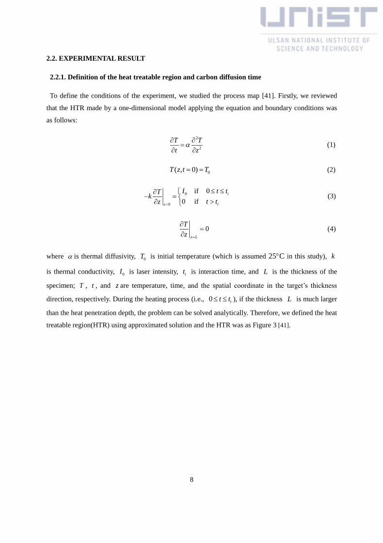
To define the conditions of the experiment, we studied the process map [41]. Firstly, we reviewed

that the HTR made by a one-dimensional model applying the equation and boundary conditions was

as follows:

2

2

T T

t z

(1)

0( , 0)T z t T (2)

0

0

if 0

0 if

i

iz

I t tTk

t tz

(3)

0z L

T

z

(4)

where is thermal diffusivity, 0T is initial temperature (which is assumed 25C in this study), k

is thermal conductivity, 0I is laser intensity, it is interaction time, and L is the thickness of the

specimen; T , t , and z are temperature, time, and the spatial coordinate in the target’s thickness

direction, respectively. During the heating process (i.e., 0 it t ), if the thickness L is much larger

than the heat penetration depth, the problem can be solved analytically. Therefore, we defined the heat

treatable region(HTR) using approximated solution and the HTR was as Figure 3 [41].

9

Figure 3. Laser HTR in terms of laser intensity and interaction time

Table 1. Material property values used for AISI 1035 [45, 46]

Thermal conductivity 50.7 W/m×K

Thermal diffusivity 1.32555×10-5

m2/s

Melting temperature 1470°C

A1 temperature 727°C

A3 temperature 793°C

Nose temperature 540°C

Once the steel is in the HTR, it needs to stay in that region long enough until the carbon fully

diffuses in austenite before it is quenched. Carbon diffusivity in austenite is a function of temperature,

and it increases with temperature. Hence, to calculate a more meaningful carbon diffusion time, the

actual temperature history must be considered with the corresponding diffusivity. In this study, a

carbon diffusivity model in austenite by Å gren [47] is adopted:

7 48339.9 1( ) 4.53 10 1 (1 ) exp 2.221 10 17767 26436c c c cD T y y y

T T

(5)

10

where cy is defined as

1

cc

c

xy

x

(6)

and cx is the mole fraction of carbon.

Normalized carbon diffusivity was defined as follows:

3

( ) ( ) /c c c AD T D T D T (7)

By integrating this normalized carbon diffusivity over the entire time duration for which the given

point stays above the A3 temperature, ECDT is defined as follows [41]:

33 3

1( ( )) ( ( ))

A A

ecd c s c s

T T T Tc A

t D T t dt D T t dtD T

(8)

In Figure 4, ECDT is plotted inside the HTR for AISI 1035 for the sum of heating and cooling

cycles. ECT as the time taken from A3 temperature to the nose temperature was suggested [41].

Before the experiment, we will predict the high hardness zone near the melting line due to carbon

diffusion time being larger than in any other region. In

Figure 4, carbon diffusion time generally consists of 5 or 6 intervals inside the HTR. Based on this

plot, we designed the Table 2 of the experiment.

11

Figure 4. Total effective carbon diffusion time (ECDT) versus interaction time (plotted for AISI 1035)

[41]

Figure 5. Effective cooling time (when it is less than 1 sec, theoretically 100% martensite can be

obtained.)

12

2.2.2. The hardness of specimen as carbon contents increased

For the experiment, a diode laser heat treatment experiment was conducted with a 3kW TRUMPF

TruDiode 3006 laser. The objectives of this experimental study are: (1) to validate the HTR, (2) to

visually present the overall hardness distributions on the laser heat treatment map in terms of laser

intensity and interaction time, and (3) to analyze the hardness distributions from the viewpoint of the

ECDT and ECT diagrams. In this study, AISI 1020 and AISI 1035 specimens are heat-treated by a

diode laser beam with a 1 cm 1 cm top-hat beam profile and 900~1000 nm wavelength. The

dimensions of each specimen are 15 cm 8 cm 3.5 cm, which are calculated considering the heat

diffusion length during the laser-on time so that boundary effects can be neglected.

Table 2. Experimental parameters and measured Shore hardness values (M denotes melted

specimens)

Exp # Interaction Time

(sec)

Laser Power

(kW)

Scanning Speed

(mm/sec)

Type D Shore

Hardness (1035)

Type D Shore

Hardness (1020)

1 0.50 1.49 20.00 21.9 20.6

2 0.50 1.91 20.00 23.4 21.9

3 0.50 2.34 20.00 42.2 25.6

4 0.50 2.76 20.00 57.2 36.5

5 0.95 1.08 10.53 21.1 20.3

6 0.95 1.39 10.53 23.8 20.4

7 0.95 1.69 10.53 48.0 28.0

8 0.95 2.00 10.53 62.3 40.6

9 0.95 2.31 10.53 68.3 50.7

10 0.95 2.61 10.53 M M

11 0.95 2.92 10.53 M M

12 1.40 0.89 7.14 21.9 19.5

13 1.40 1.14 7.14 23.9 21.9

14 1.40 1.40 7.14 36.8 24.9

15 1.40 1.65 7.14 60.0 37.5

16 1.40 1.90 7.14 66.3 52.5

17 1.40 2.15 7.14 64.3 53.7

18 1.40 2.41 7.14 M M

19 1.40 2.66 7.14 M M

20 1.40 2.91 7.14 M M

21 1.40 3.00 7.14 M M

22 2.30 0.70 4.35 22.1 22.9

23 2.30 0.89 4.35 20.7 19.2

24 2.30 1.09 4.35 23.8 22.0

25 2.30 1.29 4.35 55.4 34.6

26 2.30 1.48 4.35 64.7 48.0

27 2.30 1.68 4.35 65.8 49.8

28 2.30 1.88 4.35 M M

13

Table 2. Continued from the previous page

Exp # Interaction Time

(sec)

Laser Power

(kW)

Scanning Speed

(mm/sec)

Type D Shore

Hardness (1035)

Type D Shore

Hardness (1020)

29 2.30 2.07 4.35 M M

30 2.30 2.27 4.35 M M

31 2.30 2.47 4.35 M M

32 2.30 2.66 4.35 M M

34 3.20 0.76 3.13 21.3 19.1

35 3.20 0.92 3.13 24.6 19.5

36 3.20 1.09 3.13 55.1 26.5

37 3.20 1.26 3.13 62.5 40.8

38 3.20 1.42 3.13 63.9 51.0

39 3.20 1.59 3.13 66.9 50.8

40 3.20 1.76 3.13 M M

41 3.20 1.92 3.13 M M

42 3.20 2.09 3.13 M M

43 3.20 2.26 3.13 M M

44 4.10 0.52 2.44 22.0 21.1

45 4.10 0.67 2.44 22.6 21.6

46 4.10 0.82 2.44 22.3 19.0

47 4.10 0.96 2.44 28.2 22.8

48 4.10 1.11 2.44 50.9 29.1

49 4.10 1.26 2.44 63.1 41.1

50 4.10 1.41 2.44 63.1 54.2

51 4.10 1.55 2.44 66.4 50.3

52 4.10 1.70 2.44 M M

53 4.10 1.85 2.44 M M

54 4.10 2.00 2.44 M M

55 5.00 0.47 2.00 23.1 20.2

56 5.00 0.61 2.00 21.8 19.2

57 5.00 0.74 2.00 21.2 21.2

58 5.00 0.87 2.00 24.1 22.4

59 5.00 1.01 2.00 43.8 28.6

60 5.00 1.14 2.00 68.3 31.0

61 5.00 1.27 2.00 62.0 49.5

62 5.00 1.41 2.00 58.3 53.3

63 5.00 1.54 2.00 M M

64 5.00 1.67 2.00 M M

65 5.00 1.81 2.00 M M

66 5.00 1.94 2.00 M M

14

The details of the experiment are presented in Table 1. A set of 66 experiments covers a wide range

of interaction time from 0.5 to 5 sec and laser power up to 3 kW. For each experiment, the surface

hardness at the center of the HTR is measured ten times using a SATO Type D Shore durometer, and

the averaged hardness values are listed in Table 1. If there was clear evidence of melting, the hardness

value is replaced by a letter M in the table.

To visualize the hardness distribution on the heat treatment map, the laser power ( P ) used in the

experiment (see Table 2) needs to be converted to absorbed laser intensity ( I ). Because the laser

beam has a top-hat profile, absorbed intensity values can be calculated as:

PI

A

(9)

where is the laser beam absorptivity (which is unknown) and A is the beam area. In this study,

a laser beam absorptivity of 0.7 is assumed based on the literature [48] and the authors’ experiences.

In fact, as reported in [48], laser beam absorptivity is a function of both interaction time and laser

power, so the use of this single absorptivity value may lead to inaccurate results.

Figure 6. Measured hardness distribution for AISI 1020 (Laser absorptivity of 0.7 is assumed. Blue:

20, Green: 41, Yellow: 46, Orange: 51, Red: 56)

15

Figure 7. Measured hardness distribution for AISI 1035 (Laser absorptivity of 0.7 is assumed.

Blue: 20, Green: 42, Yellow: 57, Orange: 62, Red: 67)

Figure 6 and Figure 7 show the hardness distributions with the HTR for AISI 1020 and 1035,

respectively, where the size and color of a circle denotes the hardness at the given point. Because the

thermo-physical properties of the two steel types, such as thermal conductivity and thermal diffusivity,

are only about 2% different, the HTR for AISI 1035 can be used for AISI 1020, too.

In both figures, since the hardness values of the melted specimens are not shown on the map, the

uppermost data points represent the upper boundary line of the HTR. As seen clearly, up to the

interaction of roughly 2.5, the assumed absorptivity of 0.7 seems to be reasonable. However, at longer

interaction times, some data points lie above the HTR, and there it looks as if the actual intensity is

lower than 0.7. It is observed that near the melting temperature line, the oxidation layer gets thinner as

the interaction time increases, which explains why laser absorptivity at higher interaction times

becomes lower [48]. This agrees well with published absorptivity measurement data [48, 49], which

show that laser absorptivity decreases as laser power decreases. Considering the shape of the upper

boundary line predicted by the surface melting and the laser power dependency of absorptivity, the

one-dimensional heat conduction model seems to be reasonably good for diode laser heat treatment.

16

Observing Figure 6 and Figure 7, as expected, AISI 1035 shows a better hardening performance

than AISI 1020 under the same process conditions, which is due to higher carbon content. The overall

hardness is roughly 30% higher with a much larger area of successful heat treatment. Also, one thing

to note here is that overall hardness distributions resemble the ECDT pattern (Figure 4), rather than

the ECT pattern (Figure 5). Therefore, for the type of steels and HTR under consideration, we can say

that carbon diffusion is much more critical than cooling time. This is obvious because in Figure 5 the

ECT is less than 5 seconds for the entire HTR. Considering the TTT diagram for AISI 1020 and 1035,

5 seconds is short enough to obtain relatively high hardness provided that carbon diffusion is large

enough. On the other hand, as shown in Figure 4, ECDT varies from 0 to about 200 as the process

condition changes from the lower boundary to the upper boundary of the HTR. This explains why

heat treatment performance is poor near the lower boundary; for the given steel types, hardness

increases as the intensity increases at the same interaction time. This can be also explained in terms of

increased carbon diffusion at higher intensity (or higher temperature). For steels with poorer cooling

characteristics and good carbon diffusion characteristics, however, we believe that the hardness

distribution follows the ECT more closely.

We have also conducted a microstructural analysis of the specimens with an interaction time of 2.3

seconds using an optical microscope. In agreement with the previous hardness measurement results, a

hardened region at the surface is found only for the laser power from 1.29 kW to 1.68 kW for both the

AISI 1020 and 1035 steels. Figure 8 and Figure 9 show the optical micrographs of the AISI 1020

specimens with laser power values of 1.09 kW and 1.68 kW, respectively (see Table 2).

As seen clearly in the figures, the latter (the laser power of 1.68 kW) creates a hardened region at the

surface, but the former (1.09 kW) does not; the martensitic phase appears near the surface when the

laser power is 1.68 kW. In fact, this is in line with the measured hardness data given in Figure 6. The

same analysis has been conducted for AISI 1035 specimens, and the results are shown in Figure 10

and Figure 11. Overall the results are similar to AISI 1020, but due to the higher carbon content, more

martensite and pearlite are observed at higher laser powers compared to the AISI 1020 specimens.

17

(1) (2)


laser power of 1.09 kW. The right figure shows the magnified view of the region A in the left figure.

(1) (2)

(3) (4)

Figure 9. Optical micrographs of the AISI 1020 specimen for an interaction time of 2.3 seconds

and a laser power of 1.68 kW. Figures (2), (3) and (4) show the magnified views of the hardened zone

(A), interface zone (B), and the base zone (C) in Figure (1).

18


and a laser power of 1.09 kW. The right figure shows the magnified view of the region A in the left figure.

(1) (2)

(3) (4)


and a laser power of 1.68 kW. Figures (2), (3) and (4) show the magnified views of the hardened zone

(A), interface zone (B), and the base zone (C) in Figure (1).

19

Using the optical micrographs, we measured the hardening depth for the interaction time of 2.3

seconds. For the sake of consistency, the hardening depth is defined as the maximum distance from

the surface to the location where the martensitic phase is found, and is shown in Figure 12. As seen in

Figure 12, the martensite is found only for the three highest laser power values and the hardening

thickness increases as the laser power increases. It should be noted that the measured hardening depth

values are very close to the predicted hardening depth based on the critical ECDT.

Figure 12. Measured hardening depth vs. laser power (Interaction time: 2.3 seconds, Red: AISI

1020, Blue: AISI 1035)

2.3. REMARK

In this study, we have found how important the ECDT is in thick plate carbon steel. If carbon steel

has sufficient thickness, it accepts more martensite near the melting line and has more hardness.

Providing that we have the top-hat beam profile of the diode laser, the ECDT map proves very useful.

To develop this map, we will study other thickness carbon steel plates in the next chapter.

20

III. EFFECT OF SPECIMEN THICKNESS ON HEAT TREATABILITY

IN LASER TRANSFORMATION

3.1. INTRODUCTION

In the previous chapter, we found the importance of ECDT in laser heat treatment, although we only

considered thick plate carbon steel. Thick plates are generally used by various industries for molds,

tooling machines, and so on.

In this chapter, we investigate the effect of thickness of carbon steel on heat treatability. Recently,

there has been an increasing need for heat-treating steel sheets, but the understanding of heat

treatability for metal sheets is limited. Because of this, we studied how the laser heat treatment

process changes as the thickness of the specimen varies. In order to effectively investigate this

problem, the process map approach that was recently proposed by Ki et al. [41] has been employed in

this study, where carbon diffusion and cooling characteristics are calculated for a wide range of two

most important process parameters, i.e., laser intensity and interaction time, and are shown inside the

HTR that is defined in terms of A3 and melting temperatures of the given steel. The advantage of this

approach is that the steel type and plate thickness offer an overall perspective of the obtainable laser

heat treatment process.

Through the process, we studied the effect of specimen thickness on hardening performance in the

laser heat treatment of carbon steels and how the HTR, ECDT and ECT evolve as the thickness of the

specimen decreases from 10 cm to 1 mm.

This study shows that the HTR moves to the lower laser power side and its area decreases. Also, the

amount of carbon diffusion in the austenite phase, which we describe by using the ECDT, increases in

such a way that at 1 mm thickness, carbon diffusion is large enough for the entire process region that

we consider in this study.

We have conducted experiments using AISI 1020 specimens at four different thickness (2 cm, 1 cm, 5

mm, and 1.3 mm) using a 3 kW diode laser, and this experiment is based on HTR, ECDT, and ECT.

21


3.2.1. Definition of critical thickness and heat treatable region as thickness decreased

To define the experiment, we used the HTR considering thickness variation [50]. In Figure 13 (a)-(f),

the upper and lower boundaries for the shaded regions are defined by melting and A3 temperatures,

respectively. As seen clearly in Figure 13, there is virtually no change in the HTR as the thickness

decreases from 10 cm to 2 cm. However, when the thickness changes from 2 cm to 1 cm, the HTR starts

to deviate, starting from the high interaction time area. Therefore, we can say that the critical plate

thickness ( critL ) lies somewhere between 1 cm and 2 cm for the given problem. In other words, as far as

laser heat treatment is concerned, a plate with a thickness larger than critL can be regarded semi-infinite,

and the process map constructed for thick plates can be applied. For defining critL , Ki et al. defined the

NHTRA (normalized heat treatable region area) and the CAR (common area ratio) [50].

6

0

6

0

( , ) ( , )

NHTRA

( , ) ( , )

i

i

i

i

t

i i it

t

i i it

ub L t lb L t dt

ub L t lb L t dt

(10)

6

0

6

0

( , ) ( , )

CAR

( , ) ( , )

i

i

i

i

t

i i it

t

i i it

ub L L t lb L t dt

ub L t lb L t dt

(11)

In this study, the maximum interaction time considered in this study is 6 seconds, the heat

penetration length can be estimated as:

52 2 1.32555 10 6 0.0178 m

it

(12)

Which is very close to 15 mm, as shown in Figure 14. Also, this explains why in Figure 13 the HTR

for thin specimens starts to deviate from the large interaction time area ( 6i

t ); heat penetrates further

with a larger interaction time.

We can also notice from Figure 13 that as the thickness decreases further, the HTR deviates more,

and this deviation propagates to the lower interaction time part. As shown in Figure 13 (f), comparing

the 10 cm and 1 mm cases, the difference is huge and a completely new HTR is obtained at 1 mm

specimen thickness. Generally, as the thickness decreases, the HTR moves downward toward a lower

intensity region, which means that a much lower laser intensity is required for the laser heat treatment

of steel sheets, if heat treatment is possible. From these results, we selected the specimen thickness as

20mm, 10mm, 5mm, and 1.3mm.

22

(a) L: 10 cm 2 cm (b) L: 2 cm 1 cm

(c) L: 1 cm 5 mm (d) L: 5 mm 2.5 mm

(e) L: 2.5 mm 1 mm (f) L: 10 cm 1 mm

Figure 13. Change in HTR as a function of the plate thickness

23

Figure 14. Normalized heat treatable region area (NHTRA) vs. specimen thickness (solid line),

common area ratio (CAR) vs. specimen thickness (dashed line)

In this study, we wanted to discover whether ECDT or ECT is a more dominant factor for laser

transformation. The ECDT and ECT are shown in Figure 15 and Figure 16 [50].

As shown from the first three figures, there is not much change in the ECDT distribution up to the

plate thickness of 1.5 cm, which is reasonable considering the critical plate thickness of ~1.5 cm

calculated as mentioned previously. However, when the plate thickness is reduced to 1 cm, the upper

right side of the HTR is affected by the reduced plate thickness and shows very high values of ECDT.

Figure 16 shows how the ECT changes as the plate thickness decreases. Overall, as in the case of the

ECDT, the ECT increases as the plate thickness decreases, starting from the high interaction time and

high temperature part of the HTR.

24

(a) L = 10cm (b) L = 2cm

(c) L = 1.5cm (d) L= 1cm

(e) L = 7.5mm (f) L= 5mm

(g) L = 2.5mm (h) L = 1mm

Figure 15. Effect of plate thickness on the effective carbon diffusion time (ECDT)

25

(a) L = 10cm (b) L = 2cm

(c) L = 1.5cm (d) L = 1cm

(e) L = 7.5mm (f) L = 5mm

(g) L = 2.5mm (h) L = 1mm

Figure 16. Effect of plate thickness on the effective cooling time (ECT)

26

3.2.2. The hardness map of specimen as thickness decreased

To investigate the effect of HTR, ECDT, and ECT, we conducted a diode laser heat treatment

experiment using a 3 kW TRUMPF TruDiode 3006. That laser system has a pyrometer that is capable

of measuring surface temperature up to 1600C. In this study, AISI 1020 specimens were heat-treated

by a diode laser beam with a 0.8 cm 0.8 cm top-hat beam profile and 900~1000 nm wavelength.

To study the effect of specimen thickness on hardening performance, specimens with four different

thicknesses (20 mm, 10 mm, 5 mm, and 1.3 mm) were used. The length and width of the specimens

were 20 cm 10 cm, which were calculated considering the heat diffusion length during the laser-on

time so that boundary effects can be neglected.

A set of 125 experiments were conducted to deal with a wide range of interaction time from 1 to 4

seconds and laser power up to 2 kW with four different specimen thicknesses. For a given interaction

time, 5 to 7 different surface temperature values were selected to cover the HTR (7 temperatures for

20 and 10 mm thicknesses, 6 temperatures for 5 mm thickness, and 5 temperatures for 1.3 mm

thickness). When selecting the surface temperature values, we used 793C (A3 temperature) and

1450C (20C lower than the melting temperature) as the lower and upper boundaries, and equally

divided the interval using remaining points. The corresponding laser powers were obtained from the

laser controller unit. For each experiment, macro hardness of the surface along the centerline of the

HTR was measured five times using a Vickers hardness tester (Tukon 2100 B Tester by Intron), and

the average hardness values are listed in Table 3. Figure 17 presents the hardness distributions

together with the model-predicted HTRs (blue lines) for 20 mm, 10 mm, 5 mm, and 1.3 mm thick

specimens, where the size and color of a circle denotes the hardness at the given point.


Thickness

(mm)

Scanning speed

(mm/s)

Interaction time

(sec)

Temperature

(C)

Laser

power (W)

Average

Hardness (Hv)

20 10.00 0.8

793 993.5 138.4

903 1076.6 174.0

1012 1177.1 217.8

1122 1263.1 248.4

1231 1398.2 283.8

1341 1450.5 314.6

1450 1655.8 336.4

27


Thickness

(mm)

Scanning speed

(mm/s)

Interaction time

(sec)

Temperature

(C)

Laser

power (W)

Average

Hardness (Hv)

20

5.00 1.6

793 775.7 133.2

903 819.1 165.4

1012 892.9 210.6

1122 952.7 261.8

1231 1017.1 326.4

1341 1092.3 356.4

1450 1223.1 338.6

3.33 2.4

793 667.3 143.2

903 757.0 172.4

1012 783.4 203.0

1122 833.9 282.8

1231 893.6 339.2

1341 947.2 340.6

1450 1050.8 372.2

2.50 3.2

793 637.0 141.2

903 675.8 162.6

1012 747.0 242.8

1122 803.1 261.0

1231 835.7 301.2

1341 870 338.8

1450 987 336.8

2.0 4

793 601.5 128.8

903 686.3 236.8

1012 759.2 211.0

1122 780.3 303.0

1231 793.7 301.6

1341 847.1 332.2

1450 928.1 344.0

28


Thickness

(mm)

Scanning speed

(mm/s)

Interaction time

(sec)

Temperature

(C)

Laser

power (W)

Average

Hardness (Hv)

10

10.00 0.8

793 1021.8 156.0

903 1117.0 191.8

1012 1190.7 223.8

1122 1274.0 245.6

1231 1372.0 306.8

1341 1474.2 318.4

1450 1632.0 370.2

5.00 1.6

793 773.9 150.0

903 828.7 225.0

1012 900.8 242.4

1122 966.3 280.2

1231 1036 276.8

1341 1091.8 334.4

1450 1208.5 350.8

3.33 2.4

793 670.3 163.4

903 730.2 240.2

1012 774.0 241.6

1122 845.4 238.4

1231 889.6 284.6

1341 933.0 329.4

1450 1056.1 344.8

2.50 3.2

793 640.0 163.4

903 682.9 235.2

1012 698.3 234.8

1122 777.1 249.2

1231 809.5 280.8

1341 871.7 296.2

1450 963.7 349.6

2.00

4.0

793 599.3 168.2

903 667.9 243.2

1012 706.2 207.4

1122 739.9 265.8

1231 775.9 244.4

1341 810.3 306.4

1450 906 325

29


Thickness

(mm)

Scanning speed

(mm/s)

Interaction time

(sec)

Temperature

(C)

Laser

power (W)

Average

Hardness (Hv)

5

10.00 0.8

793 1022.3 155.0

924 1115.6 198.4

1056 1215.8 218.8

1187 1328.4 234.0

1319 1455.6 268.4

1450 1620.0 297.6

5.00 1.6

793 738.9 157.8

924 807.0 219.2

1056 881.2 233.2

1187 968.3 258.4

1319 1058.0 292.4

1450 1194.0 302.6

3.33 2.4

793 608.1 163.8

924 679.8 211.8

1056 728.8 221.4

1187 809.5 251.6

1319 874.0 268.8

1450 989.6 258.6

2.50 3.2

793 548.1 174.8

924 606.0 196.6

1056 663.3 232.8

1187 717.5 223.0

1319 790.4 242.2

1450 864.4 275.7

2.00 4.0

793 532.2 174.8

924 572.4 184.2

1056 631.9 220.4

1187 670.8 236.4

1319 702.9 242.0

1450 803.1 233.4

30


Thickness

(mm)

Scanning

speed (mm/s)

Interaction

time (sec)

Temperature

(C)

Laser

power (W)

Average

Hardness (Hv)

1.3

10.00 0.8

793 710.6 200.2

957 830.4 206.2

1122 938.8 235.6

1286 1087.8 247.2

1450 1288.0 176.6

5.00 1.6

793 397.4 193.2

957 474.4 202.8

1122 522.6 237.4

1286 703.7 229.6

1450 785.3 165.8

3.33 2.4

793 291.3 188.0

957 349.1 233.2

1122 393.1 207.2

1286 433.8 218.2

1450 501.3 213.0

2.50 3.2

793 220.2 186.6

957 264.3 209.4

1122 303.9 206.0

1286 342.3 212.2

1450 426.3 217.0

2.00

4.0

793 204.9 191.4

957 240.7 187.0

1122 272.6 226.8

1286 297.4 242.2

1450 345.0 214.2

31

(a) L = 2 cm (b) L = 1 cm

(c) L = 5 mm (d) L = 1.3 mm

Figure 17. Hardness maps for different specimen thicknesses (M denotes melted specimens.)

As shown in Figure 17, as the specimen thickness decreases, the overall hardness level decreases and

the HTR becomes narrower and moves downward toward the lower intensity region. Note that except

for the 1.3 mm case, the HTRs agree reasonably well with the experimentally determined ones [50].

As the interaction time increases, however, it seems that the model becomes less accurate as it

underestimates cooling. In other words, at longer interaction times the actual laser intensity required

to increase the temperature is higher than is predicted by the model. This is more clearly demonstrated

in Figure 17(d). We believe that the approach used in this study is effective and sufficient to

understand the effect of specimen thickness on laser heat treatment.

Another thing to be noticed from Figure 17 is that for the 20, 10, and 5 mm thick specimens, high

hardness regions are located near the melting temperature lines. This is because carbon diffusion is the

more critical factor than cooling time for these relatively thick plates, as mentioned in the previous

chapter. When the thickness is 1.3 mm, however, none of the specimens were well hardened, and we

can conclude that hardening is impossible for this thickness of AISI 1020 steel because of the

deteriorated cooling characteristic (see Figure 16). Also, comparing Figure 17 (a), (b), and (c), we can

32

notice that the interaction time where the maximum hardening occurs seems to move to the left side as

the thickness decreases (between 1.6 and 2.4 for 20 mm, to between 0.8 and 1.6 for 10 and 5 mm). We

believe that this phenomenon occurs because the high cooling time region spreads into the lower

interaction time region as the thickness decreases (see Figure 16).

In order to study the effect of thickness on hardening performance in more detail, the average

hardness for the entire hardness map (blue circles), the average hardness at 1450C (red squares), and

the average hardness at 793C (gray diamonds) are plotted versus the specimen thickness in Figure 18.

Note that the blue solid line shows the hardness of the base metal (~130 Hv). As shown in the figure,

the average hardness and the hardness at 1450C remain almost the same as the thickness changes

from 20 mm to 10 mm, but they both decrease as the thickness decreases beyond 10 mm. On the other

hand, the hardness at 793C slowly increases with thickness from a hardness value that is nearly equal

to that of the base metal. We believe that this is because, as the thickness decreases, the heating effect

lasts much longer even at the A3 temperature, and the possibility of having phase change increases.

One more interesting point is that in Figure 18, all three hardness values approach ~200 Hv as the

thickness approaches 0. In other words, as the specimen is very thin, irrespective of the heat treatment

temperature (and therefore laser power), hardness is close to 200 Hv for AISI 1020 steel. We believe

that similar hardness limits may exist for different types of steels.

Figure 18. Hardness versus specimen thickness

33

3.3. REMARK

In this study, we have found the effectiveness of HTR and the relation of ECDT and ECT. Space for

thermal conduction is necessary to obtain surface hardening performance for the sake of effective

laser transformation hardening. At this point, critL , considering the map of ECDT and ECT, is very

meaningful. If the thickness of specimen is over 1.7cm, the effect of laser transformation hardening is

equally. From the HTR, ECDT, and ECT, we can narrow the range for laser transformation hardening.

34

IV. LASER TRANSFORMATION HARDENING OF CARBON STEEL

SHEETS USING A HEAT SINK

4.1. INTRODUCTION

From chapters 2 to 3, we investigated the characteristics of carbon steel plate and know that thin

steel is very important to secure the space for thermal conduction for ECT. In this study, we suggest a

heat sink that can replace a thick plate.

The local hardening process of carbon steel sheet is very important because the use of a thinner steel

sheet that can be locally strengthened is a desirable way to reduce vehicle weight without sacrificing

the strength and safety requirements. Recently, the automotive industry has tried to apply hardening to

the body structure, but the laser hardening of thin steel is difficult, as mentioned previously.

In this chapter, we propose a laser transformation hardening technique using a heat sink as a method

to enhance the quenching performance of steel sheets. If a properly designed heat sink is used below a

steel sheet, improved cooling is expected. Thermal properties of structural steel sheets do not vary

much from one to another, but there are many options when it comes to the heat sink material.

Depending on the choice of the heat sink material and the thermal contact resistance, the heat flow

inside the specimen can be varied significantly, and various heat treatment outcomes can be obtained.

In this study, using the process map approach, the laser hardening process was studied systematically

on the intensity-interaction time diagram, on which the two main factors for the hardening process

(carbon diffusion and cooling time) and all the measurement data are presented to demonstrate in

which part of the HTR successful hardening is expected [41].

For the experiment, we used DP 590 dual phase steel and boron steel specimens with a 3 kW diode

laser with a rectangular top-hat beam profile. Note that both are specialty steels used for automotive

body parts. DP 590 steel is classified as high strength steel (HSS), and boron steel is a hot-stamping

steel that contains 10 to 30 ppm of boron as an alloying element and has a powerful hardenability.

Successful local hardening of these steels could demonstrate that this heat-sink assisted laser

hardening method can be used for manufacturing lightweight vehicles. From chapter 2 and chapter 3,

we didn’t use DP590 and boron steel in spite of this merit because both materials couldn’t be

manufactured as thick plate. Therefore, we used AISI 1020, 1035 however all of materials such as

AISI 1020, 1035 and DP590, boron steel are carbon steel, so are agreement with the purpose of this

study. For heat sink, we consider the four heat sink types had different thermal conductivity and

hardness was measured.

35


4.2.1. Definition of heat sink type

To define the experiment, we used the HTR considering thickness variation [50]. We mentioned the

map of ECDT and ECT from the previous chapter, and these maps are shown in Figure 20 and Figure

25. In this study, we used DP 590 dual phase steel with a thickness of 2mm, with the boron steel

having the same thickness.

(a) Thick steel plate (b) 2 mm steel sheet

Figure 19. Effective carbon diffusion time (ECDT) of thick steel plate and 2mm steel sheet

(a) Thick steel plate (b) 2 mm steel sheet

Figure 20. Effective cooling time of thick steel plate and 2mm steel sheet

For the specimen, the thermal properties of mild steel were used (Table 4). Note that there are many

types of carbon steels, but their thermal properties are not dissimilar. Unlike the specimen, however,

there are many choices for the heat sink material, and a proper choice may be critical for successful

hardening. Here, what characterizes a heat sink is its thermal conductivity because it determines the

36

amount of heat flow at the interface if other conditions are the same. Three heat sinks were selected

based on their thermal conductivity values: stainless steel 316, steel, and copper. Steel is considered

because, in this case, the heat sink and the specimen have basically the same thermal properties. The

only difference between this case and the hardening of a thick steel plate is the existence of thermal

contact resistance.

Table 4. Material properties of steel, stainless steel, and copper

(from MatWeb (2013) and Krauss (2005))

Steel Stainless steel 316 Copper

Thermal conductivity (W/mK) 50.7 16.3 398

Thermal diffusivity (m2/s) 1.32610

-5 4.07510

-6 1.15810

-4

Melting temperature (C) 1470 1385 1083.2

A1 temperature (C) 727 - -

A3 temperature (C) 793 - -

Nose temperature (C) 540 - -

37

4.2.2. The hardness of specimen as thermal conductivity increased

To conduct the experiment, we made the jig shown in Figure 21 which used a clamp to maintain

uniform pressure. Unfortunately, the thermal contact resistance between the specimen and the heat

sink could not be measured in this study because thermal contact resistance is influenced by many

factors, such as the type of material, surface finishing method, surface roughness, temperature, and

applied pressure [51]. In Figure 21, a specimen (purple) is placed on a heat sink (brown), which is

inserted inside a jig with six clamps. Using these clamps, both the specimen and the heat sink can be

firmly fixed during the heat treatment process.

Figure 21. Design of the experimental jig

Similar to the previous experiment described in the previous chapter, a 3 kW diode laser (TRUMPF

TruDiode 3006) was used for the hardening experiment. The laser beam has a top-hat intensity profile

with a square spot size of 5.4 mm 5.4 mm, and operates in the wavelength range of 900~1000 nm.

The focal length was 250 mm, and the beam was focused on the specimen surface. The laser heat

treatment system has a pyrometer that is capable of measuring surface temperature up to 1600C. For

the heat treatment specimens, two types of steel sheets (DP 590 dual phase steel and boron steel), with

a thickness of 2 mm were used. The chemical compositions of both steels are summarized in Table 5.

38

The size of the specimens were 200 mm 100 mm, which were calculated considering the heat

diffusion length during the laser irradiation time so that specimen boundary effects could be

minimized. For the heat sink, to be consistent with the theoretical study, four types of heat sinks (steel,

stainless steel 316, copper, and no heat sink) were considered. The thickness of the heat sink was

designed to be 30 mm, accounting for the heat diffusion length, so that the heat sink could be

considered thick during the heat treatment process.

Table 5. Chemical compositions (%) of DP 590 steel and boron steel

Steel Type C Si Mn P S B Fe

DP 590 0.078 0.0345 1.796 0.0128 0.0014 - Balance

Boron steel 0.2 0.39 1.15 0.015 0.004 0.0024 Balance

Note that the clamps on the surface may disturb the heat flow slightly, but it is believed that their

effect on the hardening process is negligibly small because they are located far away from the laser

scanning path and the primary heat flow direction is normal to the surface.

In this study, eight cases were investigated considering two specimen and four heat sink types. For

each case, a set of 24 experiments were designed to cover the process map. Therefore, the total

number of experiments conducted was 192. (24 experiments 4 heat sink types 2 steel types = 192)

To recap, the process map covered the interaction time between 0 and 2.5 s and the absorbed laser

intensity up to 3000 W. In this experimental study, four interaction time values, 0.36, 0.64, 1.13, and 2

s, were selected using a logarithmic scale, and for each interaction time six laser powers were chosen

in the following scheme. First, for a given interaction time, two laser power values were obtained

corresponding to 800C and 1400C using the pyrometer, which are close to the A3 temperature

(793C) and the melting temperature of steel (1470C). Once the two boundary laser powers were

obtained (say P1 and P4), the difference (P4 P1) was divided into three equal intervals and the

dividing (intermediate) power values (P2 and P3) were selected as P2 = P1 + (P4 P1)/3 and P3 = P2 +

(P4 P1)/3. Therefore, for a given interaction time, four laser power values were used to cover from

800C (slightly higher than the A3 temperature) to 1400C (slightly lower than the melting

temperature). In this study, the remaining two power levels were selected as P5 = P4 + (P4 P1)/3 and

P6 = P5 + (P4 P1)/3 in order to investigate the process map region right above the melting point.

39

Hardness enhancement is the single most important objective in any hardening process. In this

study, macro Vickers hardness was measured extensively for the 192 laser heat-treated specimens by

applying a load of 10 N for 15 s to investigate the effect of the hardening parameters on hardening

characteristics. Surface hardness was measured directly on the top surface of the specimen after heat

treatment. To obtain reliable measurement results, surface macro hardness along the centerline of the

HTR was measured ten times using a Vickers hardness tester (Tukon 2100B Tester by Instron), and

the average hardness was calculated. Table 6 and Table 7 show the hardness.

Table 6. Experimental parameters and measured surface temperature and macro hardness (Hv) (boron

steel)

Heat Sink

Type

Scanning Speed

(mm/s)

Beam on

Time(sec) Power(W)

Temperature

(ºC) Hardness(Hv)

No heat sink

15.00 6.67

380 800 167

533 974 284

657 1203 441

756 1400 449

903 1593 439

1027 ↑ 429

8.44 11.85

301 800 262

385 900 196

468 1110 440

552 1400 462

636 1500 473

719 ↑ 455

4.78 20.93

225 800 193

288 890 198

352 1100 481

415 1400 458

478 1500 455

542 ↑ 459

2.70 37.04

175 800 181

220 900 204

266 1100 442

311 1400 456

356 1475 451

402 ↑ 443

40


Heat Sink

Type

Scanning Speed

(mm/s)

Beam on

Time(sec) Power(W)

Temperature

(ºC) Hardness(Hv)

Heat Sink :

Stainless Steel

15.00 6.67

333 800 192

427 980 222

521 1100 535

671 1400 495

765 1550 478

859 ↑ 483

8.44 11.85

281 800 183

348 950 243

414 1125 458

496 1400 511

563 1505 462

629 ↑ 458

4.78 20.92

219 800 177

307 875 192

395 1080 480

385 1400 467

473 1520 480

561 ↑ 474

2.70 37.04

191 800 180

283 900 296

374 1075 359

319 1400 473

411 1500 479

502 ↑ 466

Heat Sink :

Steel

15 6.67

360 800 188

454 910 176

548 1130 515

624 1400 506

718 1450 482

812 1650 492

8.44 11.85

296 800 175

363 970 265

429 1125 484

512 1400 489

579 1550 487

645 ↑ 469

41


Heat Sink

Type

Scanning Speed

(mm/s)

Beam on

Time(sec) Power(W)

Temperature

(ºC) Hardness(Hv)

Heat Sink :

Steel

4.78 20.92

219 800 177

307 875 192

395 1080 480

385 1400 467

473 1520 480

561 ↑ 474

2.7 37.04

191 800 180

283 900 296

374 1075 359

319 1400 473

411 1500 479

502 ↑ 466

Heat Sink :

Steel

15 6.67

360 800 188

454 910 176

548 1130 515

624 1400 506

718 1450 482

812 1650 492

8.44 11.85

296 800 175

363 970 265

429 1125 484

512 1400 489

579 1550 487

645 ↑ 469

4.78 20.92

235 800 206

323 970 421

411 1130 523

385 1400 479

473 1500 474

561 ↑ 460

2.70 37.04

193 800 186

285 920 379

376 1180 509

323 1400 481

415 1480 485

506 ↑ 470

42


Heat Sink

Type

Scanning Speed

(mm/s)

Beam on

Time(sec) Power(W)

Temperature

(ºC) Hardness(Hv)

Heat Sink :

Copper

15

6.67 388 800 191

6.67 513 955 215

6.67 639 1025 531

6.67 681 1400 511

6.67 806 1550 496

6.67 932 ↑ 480

8.44

11.85 298 800 180

11.85 382 985 327

11.85 465 1105 474

11.85 504 1400 496

11.85 588 1520 479

11.85 671 ↑ 488

4.78

20.92 231 800 178

20.92 294 905 222

20.92 358 1100 525

20.92 397 1400 496

20.92 460 1510 474

20.92 524 ↑ 473

2.7

37.04 197 800 182

37.04 242 910 333

37.04 288 1110 519

37.04 339 1400 490

37.04 384 1520 480

37.04 430 ↑ 496

Table 7. Experimental parameters and measured surface temperature and macro hardness (Hv) (DP

590)

Heat Sink Type Scanning Speed

(mm/s)

Beam on

Time(sec) Power(W)

Temperature

(ºC) Hardness(Hv)

No heat sink 15 6.67

493 800 198

607 920 210

720 1200 325

834 1400 346

948 1540 340

1061 ↑ 337

43



(mm/s)

Beam on

Time(sec) Power(W)

Temperature

(ºC) Hardness(Hv)

No heat sink

8.44 11.85

384 800 187

451 915 208

519 1178 286

586 1400 335

653 1490 348

721 ↑ 362

4.78 20.93

281 800 175

334 950 219

386 1200 267

439 1400 332

492 1495 311

544 ↑ 313

2.70 37.04

202 800 173

241 900 195

280 1120 242

319 1400 300

358 1450 307

397 ↑ 280

Heat Sink :

Stainless Steel

15.00 6.67

486 800 194

563 970 237

639 1170 348

716 1400 352

793 1475 351

869 1605 337

8.44 11.85

341 800 186

410 1000 269

478 1170 330

547 1400 358

616 1500 333

684 ↑ 353

4.78 20.92

255 800 180

305 980 216

355 1170 333

405 1400 347

455 1480 345

505 1700 337

44



(mm/s)

Beam on

Time(sec) Power(W)

Temperature

(ºC) Hardness(Hv)

Heat Sink : Steel

15.00 6.67

481 800 199

561 980 236

641 1180 356

721 1400 375

801 1490 357

881 ↑ 342

8.44 11.85

342 800 187

406 940 234

470 1160 337

534 1400 352

598 1495 350

662 ↑ 343

4.78 20.92

251 800 193

301 925 218

352 1170 322

402 1400 352

452 1480 338

503 1695 338

2.70 37.04

205 800 175

240 950 211

275 1150 318

310 1400 334

345 1410 354

380 1510 344

Heat Sink :

Copper

15.00

6.67 519 800 199

6.67 606 890 332

6.67 694 1140 332

6.67 781 1400 374

6.67 868 1500 404

6.67 956 ↑ 353

8.44

11.85 375 800 196

11.85 438 925 217

11.85 502 1100 314

11.85 565 1400 363

11.85 628 1475 362

11.85 692 ↑ 367

45



(mm/s)

Beam on

Time(sec) Power(W)

Temperature

(ºC) Hardness(Hv)

4.78

20.92 259 800 185

20.92 310 937 228

20.92 360 1162 358

20.92 411 1400 365

20.92 462 1480 357

20.92 512 1690 346

2.7

37.04 199 800 178

37.04 241 900 215

37.04 284 1150 360

37.04 326 1400 347

37.04 368 1460 356

37.04 411 1660 336

The map of measured hardness values are presented on the I-ti diagram in Figure 23 where two sets

of mathematically calculated HTRs are also presented for comparison purposes; the green colored

region is the HTR for the thick steel plate, and the purple colored region is calculated for the 2 mm

thick steel sheet without a heat sink. Both were obtained using the map by provided Ki et al. [50].

In each figure, hardness is expressed as a circle, the size and color of which denotes the hardness

magnitude at the given point. In Figure 23, the four figures on the left are the results of boron steel,

and the four figures on the right show the results from DP 590 steel. From the first to the bottom row,

the thermal conductivity of the heat sink increases (no heat sink, stainless steel, steel, and copper).

In each hardness map in Figure 23, the distribution pattern of data points visualizes the actual HTR

corresponding to the specimen type and the heat sink type. Here, only the lowest four data points

constitute an HTR, as the top two points are designed to be above the upper boundary line. In this

study, for all eight cases (Figure 23 (a)~(h)), the HTRs obtained experimentally are located largely

between the green and purple regions, indicating that the laser hardening of steel sheets with a heat

sink is bound by the two reference hardening processes.

In Figure 23, it should be noted that the experimentally obtained HTRs deviate more from the purple

region at higher interaction times. At small interaction times, even a thin steel sheet can be considered

as a thick plate as long as the heat diffusion length is smaller than the sheet thickness.

46

As shown in Figure 23, there is virtually no hardness enhancement for the lowest two intensity levels

for all eight cases. In other words, to achieve a successful hardening, regardless of the heat sink type

and the interaction time (being considered in this study), the laser power needs to be higher than

roughly the average of P1 and P4. This result was predicted theoretically, where the ECDT for the

lower half of the HTR was found to be too small for the hardening process of carbon steel. Assuming

that the material’s thermal response is linear (or close to linear) between the A3 and melting

temperature (which is largely true because the heat equation is linear), it can be said that hardening is

not possible if the temperature is lower than the average of the A3 temperature and the melting

temperature (~1100C).

One notable thing in Figure 23 is the significant enhancement in hardness for both steels when a

heat sink is employed. The amount of hardness enhancement seems to be proportional to the thermal

conductivity of the heat sink. For both steels, the hardening performance at higher interaction times

improves as the thermal conductivity of the heat sink increases. Also, at the highest two intensity

levels, there is no significant change in surface hardness from the hardness values at the lower two

intensity levels. In other words, a notable discontinuity in hardness distributions is not recognized

across the upper boundary of the experimentally obtained HTRs.

47

Figure 22. Image of specimens of boron steel and DP590 for laser transformation hardening

48

Figure 23. The surface hardness maps of boron steel and DP590

49

As shown in Figure 23(a), as expected, boron steel shows a strong hardening capability even without

a heat sink, and it seems that a surface hardness of 450 Hv can be easily achieved without a heat sink.

With a heat sink, surface hardness higher than 500 Hv was consistently obtained regardless of the heat

sink type. For DP 590 steel sheets without a heat sink (Figure 23 (b)), hardening was more effective at

smaller interaction times (0.36 or 0.64 s), and at higher interaction times (1.13 and 2 s) hardness was

~50 Hv lower. This means that, without a heat sink, cooling is not fast enough at higher interaction

times for DP 590 steel. However, when a heat sink is used, regardless of the heat sink type, an

increase in hardness is noticed for all interaction times. Note that with a heat sink, it is now possible to

achieve 350 Hv consistently.

In order to quantitatively study the surface hardness changes due to heat sinks, for each hardness

distribution in Figure 23, the average of all 24 hardness values was calculated and presented in Figure

24. In the case of boron steel, it seems that there is a very slight decrease in hardness from steel to

copper, but it does not seem statistically meaningful. Also for DP 590 steel, from stainless steel to

steel, there is basically no increase in hardness, but hardness increases as the heat sink changes from

steel to copper. It is puzzling why the average hardness values remain almost the same for the two

cases. One possible explanation is that, for DP 590 steel, the I0-ti space used in this study may be more

optimal to stainless steel heat sink than steel heat sink. The same thing can be said of steel heat sink

(compared to copper heat sink) when it comes to boron steel.

Figure 24. Average surface hardness vs. heat sink type

50

Considering all of this, it can be said that the overall hardness level increases as the thermal

conductivity of the heat sink increases for both steels, which is due to the enhanced cooling

performance induced by the heat sinks. Note that in the theoretical part of this paper, it was revealed

that the improvement in cooling time is substantial for all three heat sink types, and is proportional to

the thermal conductivity of the heat sink. Note that for all heat sink types, boron steel has 90~110 Hv,

which makes it harder than DP 590 steel.

4.3. REMARK

In this study, laser transformation hardening of steel sheets assisted by a heat sink was investigated.

We know that when a heat sink is used, both cooling and carbon diffusion characteristics become

roughly on a par with those of the thick plate case; however, the HTR remains similar to that of the no

heat sink case.

Carbon diffusion is enough in the upper half of the HTR for all three heat sink types, and cooling

performance improves as the thermal conductivity of the heat sink increases.

Successful hardening can be obtained in the upper half of the HTRs for all three heat sink types. The

use of a heat sink is an efficient way to enhance the hardenability, and the amount of enhancement is

proportional to the heat sink’s thermal conductivity.

51

V. FINITE ELEMENT ANALYSIS OF LASER TRANSFORMATION

HARDENING PROCESS USING 3D THERMAL CONDUCTIVE

MODEL

5.1. INTRODUCTION

From chapters 2 to 4, we conducted experiments of laser transformation hardening based on a one-

dimensional heat conduction numerical model suggested from references [41]. Through the previous

studies, we conjectured the efficient laser transformation hardening process. A one-dimensional model

is very efficient in terms of cost, time, and accuracy; however, we wanted to visualize with a three-

dimensional model, simulated using AbaqusTM

software with subroutines.

There is a lot of research regarding heat treatment, cladding and welding, and cutting using

commercial software [52-56]. Although the simulation of many fields is relatively well established,

the simulation of laser heat treatment including heat sinks is yet to be studied. In this chapter, we

investigate the three-dimensional model which releases the phase mole fraction and the thermal

deformation related to the thermal expansion coefficient and phase change expansion efficient, as well

as phase transformation plasticity considering residual stress.

For this simulation we have used the user subroutines integrated into AbaqusTM

which are as follows:

- DFLUX : User subroutine to define non-uniform distributed flux in a heat transfer or mass

diffusion analysis

- FILM : User subroutine to define non-uniform film coefficient and associated sink temperatures

for heat transfer analysis

- GAPCON : User subroutine to define conductance between contact surfaces or nodes in a fully

coupled temperature-displacement analysis, coupled thermal-electrical-structural analysis, or

pure heat transfer analysis.

- USDFLD : User subroutine to redefine field variables at a material point

- UEXPAN : User subroutine to define incremental thermal strains

To conduct this simulation we used the TTT (Time-Temperature-Transformation) diagram which is

provided by Forge® software from FMK Co. The simulation process is shown in Figure 25. First, we

52

conducted the FE (finite element)-Model considering thermal conductivity, and then we checked

element type DC3D8. Second, we coded the user subroutine and simulated the heat transfer analysis.

Through the simulation, we accepted the phase mole fraction in the solid state, such as martensite,

bainite, pearlite, ferrite, and temperature history. To conduct the thermal deformation, we predefined

the temperature history at every node given the previous results of heat transfer and using the two user

subroutines (USDFLD, UEXPAN), as well as checking that element type C3D8R could accept the

result of the thermal deformation.

Figure 25. Schematic of the three dimension model simulation process

53

5.2. MATERIAL MODELING

The material behavior of steel is highly dependent on its chemical composition. The chemical

composition of steels are summarized in Table 8. The composition was used as an input for Forge® ,

which generated several material parameters. In carbon steel, the main characteristic defined the

carbon content as in Figure 26. Table 9 is calculated by the equation as follows:

3910 203 15.2 44.7 104 31.5 13.1 30 11 20 700

400 120 400

AC C Ni Si V Mo W Mn Cr Cu P

Al As Ti

(13)

3

2 2 2

912 370 27.4 27.3 6.35 37.2 95.2 190 72 64.5 5.57

332 276 485 900 16.2 . 32.3 . 15.4 . 48 . 4.32 . 17.3 .Mo

18.6Si.Ni 4.8Mn.Ni 40.5Mo.V 174C 2.46 6.86 0.322

AC C Mn Si Cr Ni V Ti Al Nb W

S P N B C Mn C Si C Cr C Ni Si Cr Si

Mn Si

2 2 2

2

9.9 1.24

60.2

Cr Mo Ni

V

(14)

1723 10.7 16.9 29.1 16.9 6.38 290AC Mn Ni Si Cr W As (15)

656 57.7 35 75 15.3 34 41.2s

B C Mn Si Ni Cr Mo (15)

561 474 33 17 17 21 10 7.5s

M C Mn Cr Ni Mo Co Si (16)

2512 452.8 16.92 14.97 9.5 71.44 . 67.62 . 216.9M C Ni Cr Mo Mn C Cr C Cs (17)

AC3 temperature uses two different rules and establishes an average from these two results [57, 58].

AC1 is computed based on [47]. The temperature BS is computed based on the Kirkaldy model [59].

Ms temperature uses two different rules and establishes an average of these two results [57, 60].

Provided properties from Forge® are shown in Table 10. Here, Tdeb is the start transformation time,

and T10% and T90% are intermediate times corresponding to the intermediate rates 10%, 90%.

Table 8. Chemical composition (%) of boron steel

Steel type C Si Mn P S B Fe

Boron steel 0.2 0.39 1.15 0.015 0.004 0.0024 Balance

54

Figure 26. Evolution of characteristic temperatures according to the carbon content around a base

content

Table 9. The Characteristic Temperature of boron steel

AC3 825.3°C

AC1 722°C

TH 574.9°C

BS 574.9°C

BF 552.5°C

Ms 421°C

Table 10. The characteristic temperature of phase (ferrite)

Ferrite : Temperature Tdeb T10% T90% Ymax

620 0.11 2.30×10-1

5.20×10-1

1.00×10-16

We draw the TTT diagram given the characteristic temperature which is shown Figure 27. In order to

calculate the phase mole fraction, the solution is calculated by the equations as follows [61-63]:

55

max

10%

90%max

10%ln(1 )

( ) ( )( )( ) ln / ln( )

90% ( ) ( )ln(1 )

( )

start

start

t T t Ty Tn T

t T t T

y T

(18)

max max

( ) ( )

10% 90%

10% 90%ln(1 ) ln(1 )

( ) ( )b( )

( ( ) ( )) ( ( ) ( ))n T n T

start start

y T y TT

t T t T t T t T

(19)

( )1 exp[ (T) ( ) ]

n Ty b t (20)

1max *

1 1 1(1 exp[ (t t) ])i

n

i i i iy y b

(21)

1

1

max

* 1

1

1ln( )

in

i

i

i

y

yt

b

(22)

To explain the process of the calculation, we made the schematic of Figure 29. Here, y is the phase

fraction, b and n are the thermos-dependent Avrami’s parameters. n is also dependent on the

nucleation mode and the form of the nucleus, is Avrami’s characteristic time defined by the

probability that a nucleus is activated. The martensite phase fraction is defined by [63]:

[1 exp( ( ))]mart aust M s

y y A M T (23)

56

Figure 27. TTT(Time-Temperature-Transformation) of boron steel

Figure 28. maximum phase fraction at temperature below AC3

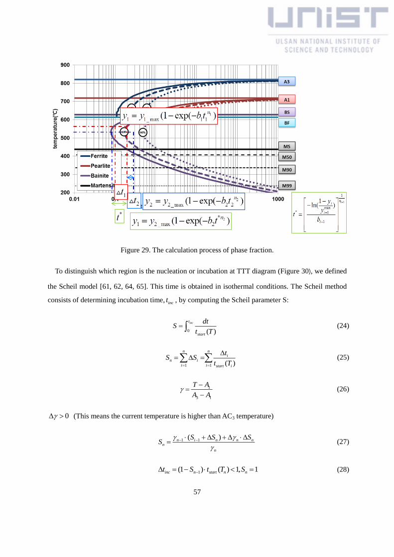
57

Figure 29. The calculation process of phase fraction.

To distinguish which region is the nucleation or incubation at TTT diagram (Figure 30), we defined

the Scheil model [61, 62, 64, 65]. This time is obtained in isothermal conditions. The Scheil method

consists of determining incubation time, inct , by computing the Scheil parameter S:

0 ( )

inct

start

dtS

t T (24)

1 1 ( )

n ni

n i

i i start i

tS S

t T

(25)

1

3 1

T A

A A

(26)

0 (This means the current temperature is higher than AC3 temperature)

1 1( )n i n n nn

n

S S SS

(27)

1(1 ) ( ) 1, 1inc n start n nt S t T S (28)

58

where inct corresponds to the transformation start time at temperature T. The beginning of

transformation for the austenite will correspond to the moment when the Scheil constant will be equal

to the unit. In other words, if nS is equal to the value of 1, the phase transformation will start. Figure

31 explains this in more detail.

Figure 30. Diagrammatic arrangement of nucleation and growth

Figure 31. Defined incubation time and Scheil model

Using the equation of incubation time, phase fraction, and Scheil model, we defined the phase

fraction which is used to accept the thermal deformation as the equation as follows [66-70]:

Thermal expansion strain tensor was defined as follows :

59

th T I (29)

1

( )phase

k k

k

y

(30)

11

22

33

0 0 1 0 0

0 0 0 1 0

0 0 0 0 1

th T

(31)

Phase change expansion strain rate tensor was defined as follows :

trtr I (32)

0

1

( )phase

tr trk k

k

y

(33)

11

22

33

0 01 0 0

0 0 0 1 0

0 0 10 0

th trk

(34)

Here, th is the thermal expansion strain tensor, is the thermal expansion coefficient and T is

the current temperature. tr is the phase change expansion strain rate tensor, ky

is the phase

change magnitude at time step. trK

is the phase change expansion coefficient.

60

Figure 32. Thermal expansion coefficient (Boron steel)

Figure 33. Phase change expansion coefficient (Boron steel)

0 200 400 600 800 1000 12000.000000

0.000005

0.000010

0.000015

0.000020

0.000025

0.000030

Th

erm

al

exp

an

sio

n c

oef

fici

ent

(1/o

C)

Temperature (oC)

Austenite

Ferrite, Pearlite

Bainite, Martensite

0 200 400 600 800 1000 12000.000

0.003

0.006

0.009

Phas

e c

han

ge

expan

sion c

oef

fici

ent

Temperature (oC)

Ferrite

Pearlite, Bainite, Martensite

61

5.3. 3D SIMULATION

5.3.1. Process of user subroutine.

To conduct this study, we defined the solutions of the phase fraction and thermal deformation. After

that, we used the material model which made the user subroutine such as DFLUX, FILM, USDFLD,

and UEXPAN, and in the case of using a heat sink, we used the user subroutine of GAPCON.

Considering the two neighboring computational cells at the material interface shown in Figure 34, the

heat flux q can be calculated [51] as:

( / 2) ( / 2)

s

T Tq

z zR

k k

(35)

where, T

and T

are temperatures at the specimen side and the heat sink side, respectively, and

R and z are thermal contact resistance and grid spacing, respectively.

Figure 34. Schematic diagram of the laser transformation hardening process and two neighboring

computational cells. [50]

In the first step, we conducted the heat transfer analysis, and for the sake of this simulation, we initially

defined the laser heat source using DFLUX and with FILM, we defined the general condition of

convection. Secondly, USDFLD defined the phase fraction. USDFLD is able to define new solution-

dependent material properties called STATEV(NSTATV) which is an array containing the solution-

dependent state variables. These are passed in as the values at the beginning of the increment. In all cases,

62

STATEV(NSTATV) can be updated in this subroutine, and the updated values are passed into other user

subroutines (CREEP, HETVAL, UEXPAN, UMAT, UMATHT, and UTRS) that are called at this material

point [71] and NSTATV means a user-defined number of solution-dependent state variables.

In this study, we defined the STATEV(NSTATV), respectively. STATEV(1) is the austenite fraction,

STATEV(2) is the ferrite fraction, STATEV(3) is the pearlite fraction, STATEV(4) is the bainite

fraction, STATEV(5) is the martensite fraction, STATEV(6) is the temperature, and STATEV(7) is

Scheil’s parameter.

USDFLD can call utility routine GETVRM to access material point data. GETVRM makes it

possible to access the temperature and stress. To obtain ferrite, pearlite, and bainite, we defined the

user subroutine process in Figure 35. In Figure 35, f

T ,p

T and b

T are the phase fraction evolution

times corresponding to ferrite, pearlite, and bainite, respectively. In the case of using the heat sink,

GAPCON is applied. For the next step (general static analysis), an additional temperature output file

(*.fil : file type) was created.

In the second step, we conducted the general static analysis to predefine the temperature at every

node of the previous heat transfer analysis. In this step, at first we defined the USDFLD to be the

same as the previous step, and in USDFLD, we defined the thermal expansion as STATEV(8). In

UEXPAN, STATEV(8) multiplies the temperature increment per every time step, and we accepted the

thermal deformation applied thermal expansion and phase transformation.

Figure 35. Calculation of ferrite, pearlite, martensite

63

5.3.2. Result of the simulation

To conduct the simulation, we considered the experiment conditions provided by the authors [40]. A

laser power ( P ) was converted to absorbed laser intensity ( I ) as:

beamPI

A

(36)

where beam

is the laser beam absorptivity and A is the beam area. However, in this study, we did

not consider the value of beam

, but simply used the real intensity which was the same value as

measured laser power of experiment in chapter 4. We wanted to know the tendency of the laser

transformation hardening regarding the effect of the heat sink and thermal contact resistance. Heat

flux was defined by equations (1)-(3). Heat flux is defined by a diode laser beam with a 5.4 mm 5.4

mm top-hat beam profile. The material of the specimen is boron steel, which contains 24 ppm of

boron as an alloying element.

Convection and radiation are considered negligible in this study, but a more advanced study should

include convection and radiation. The mesh size of the FE-Model and the time step is defined by mesh

convergence, as shown in Figure 36.

Figure 36. FE-Model of specimen and heat sink

64

The phase fractions are achieved by heat transfer analysis which is simulated by AbaqusTM

using

user subroutines such as DFLUX (for heat flux), FILM (for convection), GAPCON (for thermal

contact resistance), and USDFLD (for phase fraction). For the simulation, the boundary condition

used is shown in Table 11 where the interaction time is 0.64sec.

Table 11. The simulation conditions (boron steel no heat sink type)

Scanning speed (mm/s) Beam on time(sec) Intensity(W/cm2)

8.44 11.85

1,032

1,319

1,606

1,893

2,180

Firstly, we conducted the case of no heat sink. Before identifying the phase fraction, we checked the

temperature history at a given point, as shown in Figure 37. This figure is similar to a one-

dimensional model [50], and from this graph, we could predict the phase type partially.

Figure 37. Time history (Intensity is 1317(W/cm2)and Interaction time is (0.64sec))

In this study, the phase fraction is defined by SDV(N) as Table 12.

0 1 2 3 4 50

100

200

300

400

500

600

700

Tem

per

atu

re (

oC

)

Time (sec)

Temperature

65

Table 12. Define SDV(N)

SDV(N) Phase

SDV(1) Austenite

SDV(2) Ferrite

SDV(3) Pearlite

SDV(4) Bainite

SDV(5) Martensite

Figure 39 shows the phase fraction by intensity, respectively. In Figure 39, we investigated that the

phase fraction agrees with the theoretical phenomenon. In Figure 39 (a), we could not see the phase of

austenite, bainite, or martensite because the temperature does not reach AC1 or AC3, and in Figure 39

(b), we could find the martensite, but the hardening depth is very low because one gradation is 0.5mm,

which indicates scarcely obtaining transformation hardening. In Figure 39(b), the maximum amount

of martensite is 100%, and there are no other phases as expected. In Figure 39 (c)~(i), we can find that

the hardening depth becomes dramatically deeper as intensity increases, and the bainite fraction

increases more as intensity increases. On the other hand, the martensite fraction decreases as intensity

increases. That indicates the cooling rate is as slow as that of intensity, and that the space for thermal

conduction is not sufficient, as already mentioned [40, 50].

We can find the martensite located either side of the specimen. The reason for this phenomenon is

the cooling process. To explain this, we attached the cooling process of laser transformation hardening

as an intensity of 1,606W/cm2.

Figure 40 shows the temperature history of node 1, 2. Node 1 was the location had martensite phase

and node 2 was the location had bainite and martensite. In

Figure 40, the cooling time of node 1 from AC3 to Ms is 1.01sec and the cooling time of node 2 is

1.24sec that is the reason why generates the martensite fraction and the bainite fraction.

The reason of low hardness in the no heat sink case despite high intensity is predicted by much

bainite in terms of phase transformation hardening. In Figure 39 (d), the maximum bainite fraction is

0.6, and from Figure 39 (f), the maximum value of the bainite fraction is 1.0. That denotes why the

hardness is low in spite of the deep hardening depth.

66

Figure 38. Temperature gradient at laser moving (I = 1606W/cm2)

(a) No phase change (I=1032W/cm

2)

(b) Martensite fraction (I=1319W/cm

2)

(c) Bainite fraction (I=1606W/cm

2)

(d) Martensite fraction (I=1606W/cm

2)

(e) Bainite fraction (I=1893W/cm

2)

(f) Martensite fraction (I=1893W/cm

2)

67

(g) Martensite fraction (I=2180W/cm

2)

(h) Bainite fraction (I=2180W/cm

2)

Figure 39. The phase fractions by intensity, respectively (ti=0.64s)

Figure 40. Temperature history of node (1) and node(2)

From the simulation of carbon steel sheet, we could conjecture the phenomenon of phase

transformation and agree with the result of the experiment of the one-dimensional model. As

68

mentioned in previous chapters, we simulated the effect of a heat sink. Four types of heat sink were

selected: mild steel, stainless steel, copper, and no heat sink. Similar to the no heat sink type, we

conducted the simulation of heat transfer analysis. In this study, we added the user subroutine of

GAPCON for the sake of thermal contact resistance. The variation of thermal contact resistance is R =

510-6

m2K/W, R = 510

-5 m

2K/W and R = 510

-4 m

2K/W [40]. For simulation, firstly we checked the

temperature history of the heat sink, and compared it to the tendency of the result of the one-

dimensional model [40]. We confirmed the validation of GAPCON from the temperature profile as

the vertical direction comparing the one-dimensional model, as in Figure 41. In Figure 41, we only

want to know the tendency, so the values of the intensity and interaction time do not matter.

(a) 3D model (I=1032W/cm2, ti=0.64s) (b) 1D model (I=1600W/cm

2, ti=0.5s)

Figure 41. Tendency of temperature profile according to thermal contact resistance

The 3D simulation actually spends too much time on a solution for just one model, and our objective

is the difference of the changed thermal contact resistance. Therefore, we determined the value as the

reference of the experiment result in chapter 3. Table 13 shows the simulation parameters as changing

heat sink types, and the value of intensity is different, but which is defined as the same temperature

(1400oC) measured in the experiment as referenced in Table 6.

Table 13. The simulation condition as three heat sink type

Heat sink type Scanning speed (mm/s) Beam on time(sec) Intensity(W/cm2)

Stainless steel 8.44 11.85 1,701

Steel 8.44 11.85 1,756

Copper 8.44 11.85 1,728

69

Figure 42 shows the contour of the temperature with changed thermal contact resistance, and it

agrees with Figure 41. The thermal conduction increases with decreased thermal contact resistance, as

expected.

(a)Stainless steel(R = 510-4

m2K/W)

(b) Stainless steel(R = 510-5

m2K/W)

(c) Stainless steel(R = 510-6

m2K/W)

Figure 42. Temperature contour as changed thermal contact resistance (I=1701W/cm2ti=0.64s)

The four types of heat sink affect the phase fraction due to cooling time and carbon diffusion time.

Thus, we confirmed the phase fraction of each of the specimens as changing thermal contact

resistance. Figure 43 shows the phase fraction regarding different intensity, but with the same

interaction time, and the same temperature. When we used the stainless steel heat sink, the hardening

depth decreased as thermal contact resistance decreased. The most important factor in this

phenomenon is that the maximum temperature of low thermal contact resistance is lower than that of

high thermal contact resistance. That means that the high intensity is needed for the sake of enhancing

70

laser transformation hardening. In this case, the point is that there appears no bainite fraction that

denotes the thermal conductivity, and the cooling rate is higher than the no heat sink type. This

phenomenon occurred for the different heat sink types. In Figure 44 (c), the maximum martensite

fraction is 79%, meaning the maximum temperature is higher than AC1 and lower than AC3.

Considering the thermal conductivity and cooling rate, low thermal contact resistance and high

intensity obtains high hardening performance. In Figure 45(c), there is no change in phase fraction.

When we check the temperature, the maximum temperature is lower than AC1. Considering the phase

fraction for the four heat sink types—no heat sink, stainless steel, steel, and copper—we agree with

the phenomenon of the experiment’s result [72]. Figure 46 shows optical micrographs regarding

hardening depth being equal to the demonstration of the analysis of the experiment [72], and we will

conjecture that the thermal contact resistance is over 510-4

(m2K/W) considering hardening depth.

After we decided value of the thermal contact resistance, which is 510-4

(m2K/W) and we conducted

the simulation from I1 to I5 for the sake of analysis of phase fraction.

Figure 47 shows the phase fraction with changing heat sink type and intensity. In Figure 47, in the

case of the no heat sink type, we could not accept the martensite phase, but when the heat sink is

employed, we have the martensite at nearly 100% regardless of the heat sink type. Note that by

employing a heat sink, martensite formation can be promoted due to increased temperature gradient

near the specimen surface. That means the heat sink is very useful in accepting the martensite in spite

of high thermal contact resistance.

In Figure 47, the lowest level intensity does not reach the AC1 temperature, so there is no phase

change. For the lowest intensity level (I1), in most cases hardening did not take place, which implies

that any thermal deformation for these two intensity levels are due to plastic deformation, not because

of microstructural change. At the same intensity levels, the performance of phase change is different,

which is caused by a heat sink which is as though the effective heat input is decreased, which results

in a decrease in the deformation angle. As reported in literature [73], the plastic deformation angle is

proportional to the amount of heat input.

71

(a) Martensite (R = 510-4

m2K/W) (maximum : 100%)

(b) Martensite (R = 510-5


(c) Martensite (R = 510-6


Figure 43. Phase fraction used the stainless steel heat sink as decreased thermal contact

resistance (I = 1701W/cm2, ti = 0.64s)

(a) Martensite(R = 510-4


(b) Martensite(R = 510-5


(c) Martensite(R = 510-6


Figure 44. Phase fraction used the steel heat sink as decreased thermal contact resistance

(I =1756W/cm2, ti=0.64s)

72

(a) Martensite(R = 510-4


(b) Martensite(R = 510-5

m2K/W) (maximum : 98.5%)

(c) No phase change (R = 510-6

m2K/W)

Figure 45. Phase fraction used the copper heat sink as decreased thermal contact resistance

(I =1728W/cm2, ti=0.64s)

Figure 46. Optical micrographs showing the cross-sections of heat treated boron steel specimens for

ti = 1.13 s. From bottom to top, intensity level increases from I1 to I6. (from Kim et al[2015])

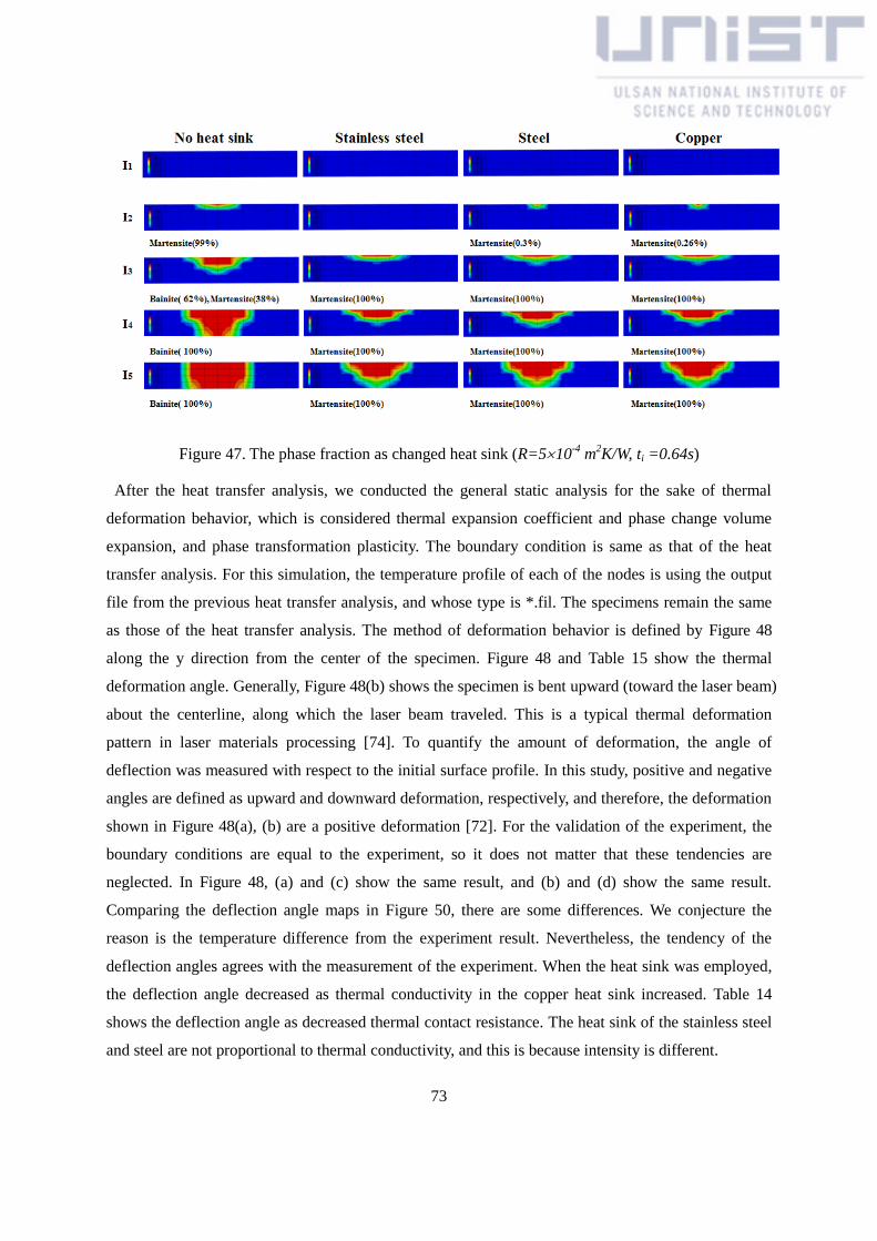
73

Figure 47. The phase fraction as changed heat sink (R=510-4

m2K/W, ti =0.64s)

After the heat transfer analysis, we conducted the general static analysis for the sake of thermal

deformation behavior, which is considered thermal expansion coefficient and phase change volume

expansion, and phase transformation plasticity. The boundary condition is same as that of the heat

transfer analysis. For this simulation, the temperature profile of each of the nodes is using the output

file from the previous heat transfer analysis, and whose type is *.fil. The specimens remain the same

as those of the heat transfer analysis. The method of deformation behavior is defined by Figure 48

along the y direction from the center of the specimen. Figure 48 and Table 15 show the thermal

deformation angle. Generally, Figure 48(b) shows the specimen is bent upward (toward the laser beam)

about the centerline, along which the laser beam traveled. This is a typical thermal deformation

pattern in laser materials processing [74]. To quantify the amount of deformation, the angle of

deflection was measured with respect to the initial surface profile. In this study, positive and negative

angles are defined as upward and downward deformation, respectively, and therefore, the deformation

shown in Figure 48(a), (b) are a positive deformation [72]. For the validation of the experiment, the

boundary conditions are equal to the experiment, so it does not matter that these tendencies are

neglected. In Figure 48, (a) and (c) show the same result, and (b) and (d) show the same result.

Comparing the deflection angle maps in Figure 50, there are some differences. We conjecture the

reason is the temperature difference from the experiment result. Nevertheless, the tendency of the

deflection angles agrees with the measurement of the experiment. When the heat sink was employed,

the deflection angle decreased as thermal conductivity in the copper heat sink increased. Table 14

shows the deflection angle as decreased thermal contact resistance. The heat sink of the stainless steel

and steel are not proportional to thermal conductivity, and this is because intensity is different.

74

With decreasing thermal contact resistance, the deflection angles decreased. Table 15 shows the

deflection angle with changing heat sink type. Figure 50 shows the tendency for thermal deformation

as four types of heat sink. Obviously, when the heat sink is used, thermal deformation decreases and

initially small positive deflection angles become negative, making it possible to find laser parameters

that lead to virtually no thermal deformation.

(a) Contour of thermal deformation(I = 2180W/cm2, Scale factor = 50)

(b) Schematic of thermal deformation(I = 2180W/cm2)

Figure 48. The measurement of thermal deformation behavior in 3D model, no heat sink type

(boron steel, ti = 0.64s)

75

Table 14. Deflection angles with changed thermal contact resistance from the 3D model

Type Thermal contact resistance

(m2K/W)

Intensity

(W/cm2)

Deflection angle(o)

Heat sink : stainless steel

510-4

1,701

0.284º

510-5

0.297º

510-6

0.399º

Heat sink : steel

510-4

1,756

0.180º

510-5

0.290º

510-6

0.411º

Heat sink : copper

510-4

1,728

0.303º

510-5

0.442º

510-6

0.452º

Table 15. Thermal deflection angles in four heat sink type from the 3D model

Type Thermal contact resistance

(m2K/W)

Intensity

(W/cm2)

Deflection angle(o)

No heat sink -

1,032 0.147 º

1,319 0.247 º

1,606 0.200 º

1,893 0.644 º

2,180 1.780 º

Heat sink : stainless

steel 510

-4

964 0.156 º

1,209 0.196 º

1,455 0.260 º

1,701 0.284 º

1,947 0.561 º

Heat sink : steel 510-4

1,015 0.160 º

1,262 0.211 º

1,509 0.248 º

1,756 0.180 º

2,003 0.714 º

Heat sink : copper 510-4

1,022 0.158 º

1,257 0.231 º

1,493 0.251 º

1,728 0.303 º

1,964 0.589 º

76

Figure 49. The map of deflection angles with changing heat sink type

77

(a) No heat sink (b) Stainless steel heat sink

(c) Steel heat sink (d) Copper heat sink

Figure 50. Deflection angle maps (boron steel)(from Kim et al[2015])

5.4. REMARK

We conducted a simulation of a three-dimensional model and predicted the phase fractions and the

thermal deformation behavior during laser transformation hardening. Even though the simulation of

the three-dimensional model consumed a lot of time, which is anticipated as the good predicted model

to analyze the phase fraction and thermal deformation behavior. In this study, we found how effective

the one-dimensional model provided by Ki et al. [40] is in reducing simulation time.

Although we already demonstrated the effect of heat sink from the experiments, we realized the

process of phase transformation for laser transformation hardening.

78

VI. CONCLUSION

This thesis presented overall laser transformation hardening of carbon steel sheets and proposed the

method of enhancing surface hardening as various approaches. In addition, the usefulness of the

predicted one-dimensional model was demonstrated by the experiment, and the three-dimensional

model could predict the process of laser transformation hardening phenomenon. Some conclusions

have been derived to demonstrate the usefulness of this study in each chapter.

First, we investigated the map of the HTRs, ECDT, and ECT, and from the experiment of the thick

plate laser transformation hardening, as carbon steel contained a different carbon fraction. We found

that carbon diffusion time is a more important factor than carbon cooling time for laser transformation

hardening.

Secondly, we investigated the difference of the HTRs, ECDT, and ECT when thickness decreases.

In chapter 2, we found the critical thickness changed the HTR with decreasing thickness, and we

found that carbon cooling time is a more important factor than carbon diffusion time. We accepted the

idea about the heat sink instead of something else for decreasing the carbon cooling time.

Third, we demonstrated the effectiveness of the heat sink for the sake of enhancing surface

hardening. We found that laser transformation hardening has better performance with increasing

thermal conductivity and decreasing thermal contact resistance. Unfortunately, we could not measure

the thermal contact resistance, but we could predict the thermal contact resistance through the one-

dimensional model.

Lastly, we could predict the phenomenon of phase fraction and thermal deformation behavior

during laser transformation hardening because of the three-dimensional model. The three-dimensional

model could be understood and predict the cause of the experiment result and the usefulness of the

one-dimensional model. Furthermore, when a heat sink is used, the decrease in thermal deformation is

caused by decreased plastic deformation due to decreased heating, and this promotes martensite

formation due to the enhanced cooling effect.

The last enhancement for this experiment approach is what controls the thermal contact resistance

and cooling rate. To complete the three-dimensional model needs accurate properties from the

experiment considered in the phase expansion and phase change expansion. Finally, we were able to

make the complete model considering changing grain size during laser transformation hardening.

79

REFERENCES

1. Kannatey-Asibu Jr, E., Principles of laser materials processing. Vol. 4. 2009: John Wiley &

Sons.

2. Kusinski, J., et al., Laser modification of the materials surface layer–a review paper. Bulletin

of the Polish Academy of Sciences: Technical Sciences, 2012. 60(4): p. 711-728.

3. Maiman, T.H., Stimulated optical radiation in ruby. 1960.

4. Koechner, W., Solid-state laser engineering. Vol. 1. 2006: Springer.

5. Bertolotti, M., The history of the laser. 2004: CRC press.

6. http://en.wikipedia.org/wiki/C._Kumar_N._Patel.

7. Majumdar, D. and I. Manna, Laser material processing. International Materials Reviews,

2011. 56(5-6): p. 341-388.

8. Li, L., The advances and characteristics of high-power diode laser materials processing.

Optics and Lasers in Engineering, 2000. 34: p. 231-253.

9. Kim, J.-D. and U. Tamotsu, Recent Topics on Laser Processing in Japan. J. of Welding and

Joining, 2008. 26(4).

10. Corp., T., Advances in High Power Lasers_TRUMPF.

11. http://www.coherent.com, Heat Treating with High Power Diode Lasers.

12. Bonss, S., et al., Precise hardening with high power diode lasers using beam shaping mirror

optics. High-Power Diode Laser Technology and Applications, 2003. 4973.

13. Krattley, D. and P. INC., Utilization of High Power Fiber, Disc, and Diode Lasers for

Welding, Heat Treating, and Cladding of Metals. IMTS Conference Presentation, 2012.

14. Babu, P.D., K. Balasubramanian, and G. Buvanashekaran, Laser surface hardening: a review.

International Journal of Surface Science and Engineering, 2011. 5(2): p. 131-151.

15. Ready, J.F., D.F. Farson, and T. Feeley, LIA handbook of laser materials processing. 2001:

Laser Institute of America Orlando.

16. Vilar, R., R. Colaco, and A. Almeida, Laser surface treatment of tool steels. Optical and

http://en.wikipedia.org/wiki/C._Kumar_N._Patel

http://www.coherent.com/

80

quantum electronics, 1995. 27(12): p. 1273-1289.

17. Chen, S.-L. and D. Shen, Optimisation and quantitative evaluation of the qualities for Nd-

YAG laser transformation hardening. The International Journal of Advanced Manufacturing

Technology, 1999. 15(1): p. 70-78.

18. Pereira, A., et al., XeCl laser treatment of steel surface. Applied surface science, 2002. 197: p.

845-850.

19. Chen, T., et al., A study on austenite transformation during laser heating. Journal of

materials processing technology, 1997. 63(1): p. 546-549.

20. Chen, W., C. Roychoudhuri, and C.M. Banas, Design approaches for laser-diode material-

processing systems using fibers and micro-optics. Optical Engineering, 1994. 33(11): p. 3662-3669.

21. Kugler, P., P. Hoffman, and M. Geiger. Low cost laser system for material processing. in

ICALEO'98. 1998.

22. Kim, J., et al., Heat Treatment Characteristics of a Press Draw Mold by Using High Power

Diode Laser. J. of the Korean Society for Heat Treatment, 2009. 22(6): p. 339-344.

23. Hwang, H.-T., S.-W. So, and J.-D. Kim, Combined Heat Treatment Characteristics of Cast

Iron for Mold Materials. The Korean Journal of Metals and Materials, 2011. 21: p. 7.

24. Hwang, H.-T., S.-W. So, and J.-D. Kim, A Study on Hardening Characteristics of Carbon

Steel by Using Finite Element Method. J. of the Korean Society for Heat Treatment, 2011. 24(4): p.

203-208.

25. Dobrzański, L., et al., Application of high power diode laser (HPDL) for alloying of

X40CrMoV5-1 steel surface layer by tungsten carbides. Journal of Materials Processing Technology,

2004. 155: p. 1956-1963.

26. Pashby, I., S. Barnes, and B. Bryden, Surface hardening of steel using a high power diode

laser. Journal of Materials Processing Technology, 2003. 139(1): p. 585-588.

27. Willam M. Steen, J.M., Laser Material Processing 4th Edition.

28. Lopez, V., et al., Surface laser treatment of ductile irons. Journal of materials science, 1994.

29(16): p. 4216-4224.

81

29. Selvan, J.S., K. Subramanian, and A. Nath, Effect of laser surface hardening on En18 (AISI

5135) steel. Journal of Materials Processing Technology, 1999. 91(1): p. 29-36.

30. Kovalenko, V.S. and D.F. Dauw, Ways to intensify laser hardening technology. CIRP Annals-

Manufacturing Technology, 1998. 47(1): p. 133-136.

31. Woo, H. and H. Cho, Estimation of hardened layer dimensions in laser surface hardening

processes with variations of coating thickness. Surface and Coatings Technology, 1998. 102(3): p.

205-217.

32. Gutu, I., et al., Surface treatment with linearly polarized laser beam at oblique incidence.

Optics & Laser Technology, 2002. 34(5): p. 381-388.

33. Pokhmurs' ka, H., Strength of cylindrical specimens subjected to laser hardening along the

generator and a spiral path. Materials Science, 2002. 38(1): p. 99-103.

34. Rozzi, J.C., F.P. Incropera, and Y.C. Shin, Transient, three-dimensional heat transfer model

for the laser assisted machining of silicon nitride: II. Assessment of parametric effects. International

Journal of Heat and Mass Transfer, 2000. 43(8): p. 1425-1437.

35. Komanduri, R. and Z. Hou, Thermal analysis of the laser surface transformation hardening

process. International Journal of heat and mass transfer, 2001. 44(15): p. 2845-2862.

36. Cho, H.Y., et al., Finite element analysis for surface hardening of SM45C round bar by diode

laser. The Korean Society of Mechanical Engineers, 2007. 5: p. 784-789.

37. Lakhkar, R.S., Y.C. Shin, and M.J.M. Krane, Predictive modeling of multi-track laser

hardening of AISI 4140 steel. Materials Science and Engineering: A, 2008. 480(1): p. 209-217.

38. Kong, F., S. Santhanakrishnan, and R. Kovacevic, Numerical modeling and experimental

study of thermally induced residual stress in the direct diode laser heat treatment of dual-phase 980

steel. The International Journal of Advanced Manufacturing Technology, 2013.

39. Meijer, J. and I. van Sprang, Optimization of Laser Beam Transformation Hardening by One

Single Parameter. CIRP Annals - Manufacturing Technology, 1991. 40(1): p. 183-186.

40. Hyungson Ki, S.S., Sanseo Kim, Laser transformation hardening of carbon steel sheets

using a heat sink. Journal of Materials Processing Technology, 2014: p. 2693-2705.

41. Ki, H. and S. So, Process map for laser heat treatment of carbon steels. Optics & Laser

82

Technology, 2012. 44(7): p. 2106-2114.

42. Mazumder, J., Laser heat treatment: the state of the art. JOM, 1983. 35(5): p. 18-26.

43. Kou, S., D. Sun, and Y. Le, A fundamental study of laser transformation hardening.

Metallurgical Transactions A, 1983. 14(3): p. 643-653.

44. Billur, E. and T. Altan, Challenges in forming advanced high strength steels. Proceedings of

New Developments in Sheet Metal Forming, 2012: p. 285-304.

45. Krauss, G., Steels: Processing, Structure, and Performance. USA: ASM International, 2005.

46. http://www.matweb.com.

47. Å gren, J.,

Scripta metallurgica, 1986. 20(11): p. 1507-1510.

48. Pantsar, H. and V. Kujanpää, Diode laser beam absorption in laser transformation hardening

of low alloy steel. Journal of laser Applications, 2004. 16(3): p. 147-153.

49. Pantsar, H. and V. Kujanpaa, Diode laser beam absorption in laser transformation hardening

of low alloy steel. Journal of Laser Applications, 2004. 16(3): p. 147-153.

50. So, S. and H. Ki, Effect of specimen thickness on heat treatability in laser transformation

hardening. International Journal of Heat and Mass Transfer, 2013. 61: p. 266-276.

51. Cengel, Y., Introduction to Thermodynamics and Heat Transfer+ EES Software. 2007: New

York: McGraw Hill Higher Education Press.

52. Aydiner, C.C., Investigation of thermal tempering in bulk metallic glasses, 2004, California

Institute of Technology.

53. De Deus, A.M., A thermal and mechanical model of laser cladding. Dissertation Abstracts

International, 2004. 65(04).

54. Drezet, J.-M., et al. Modelling the Marangoni convection in laser heat treatment. in Journal

de Physique IV (Proceedings). 2004. EDP sciences.

55. Santhanakrishnan, S., F. Kong, and R. Kovacevic, An experimentally based thermo-kinetic

phase transformation model for multi-pass laser heat treatment by using high power direct diode laser.

The International Journal of Advanced Manufacturing Technology, 2012. 64(1-4): p. 219-238.

http://www.matweb.com/

83

56. Laitinen, A., Two-dimensional simulation of thermal cutting of low-alloyed steels. 2015.

57. Andrews, K., Empirical formulae for the calculation of some transformation temperatures. J.

Iron Steel Inst, 1965. 203(7): p. 721-727.

58. Kasatkin, O., B. Vinokur, and V. Pilyushenko, Calculation models for determining the

critical points of steel. Metal Science and Heat Treatment, 1984. 26(1): p. 27-31.

59. Kirkaldy, J. and D. Venugopalan, Prediction of microstructure and hardenability in low-alloy

steels. Phase Transformations in ferrous alloys, 1983: p. 125-148.

60. Steven, W. and A. Haynes, The temperature of formation of martensite and bainite in low-

alloy steels. Journal of the Iron and Steel Institute, 1956. 183(8): p. 349-359.

61. Avrami, M., Kinetics of phase change. I General theory. The Journal of Chemical Physics,

1939. 7(12): p. 1103-1112.

62. Joshnson, W. and P. Mehl, Reaction kinetics in processes of nucleation and growth. Trans

Amer Inst Mining (Metal) Engrs, 1939. 135: p. 416.

63. Koistinen, D. and R. Marburger, A general equation prescribing the extent of the austenite-

martensite transformation in pure iron-carbon alloys and plain carbon steels. acta metallurgica, 1959.

7(1): p. 59-60.

64. Avrami, M., Kinetics of phase change. II transformation‐time relations for random

distribution of nuclei. The Journal of Chemical Physics, 1940. 8(2): p. 212-224.

65. Avrami, M., Granulation, phase change, and microstructure kinetics of phase change. III.

The Journal of chemical physics, 1941. 9(2): p. 177-184.

66. Denis, S., S. Sjöström, and A. Simon, Coupled temperature, stress, phase transformation

calculation. Metallurgical Transactions A, 1987. 18(7): p. 1203-1212.

67. Aliaga, C., Simulation numérique par éléments finis en 3D du comportement

thermomécanique au cours du traitement thermique d'aciers: application à la trempe de pièces

forgées ou coulées, 2000, École Nationale Supérieure des Mines de Paris.

68. Leblond, J., J. Devaux, and J. Devaux, Mathematical modelling of transformation plasticity

in steels I: case of ideal-plastic phases. International journal of plasticity, 1989. 5(6): p. 551-572.

84

69. Leblond, J., Mathematical modelling of transformation plasticity in steels II: coupling with

strain hardening phenomena. International journal of plasticity, 1989. 5(6): p. 573-591.

70. Videau, J.-C., G. Cailletaud, and A. Pineau, Modélisation des effets mécaniques des

transformations de phases pour le calcul de structures. Le Journal de Physique IV, 1994. 4(C3): p.

C3-227-C3-232.

71. Simulia, Abaqus 6.11, User Subroutines Reference Manual

72. Kim, S., S. So, and H. Ki, Controlling thermal deformation using a heat sink in laser

transformation hardening of steel sheets. Journal of Materials Processing Technology, 2015. 216: p.

455-462.

73. Lawrence, J., M.J. Schmidt, and L. Li, The forming of mild steel plates with a 2.5 kW high

power diode laser. International Journal of Machine Tools and Manufacture, 2001. 41(7): p. 967-977.

74. Steen, W.M., Mazumder, J., Laser material processing. Springer-Verlag, London, 2010. 4th

ed.

85

ACKNOWLEDGEMENT

Until completing this thesis, there are many trials and failures. However, when I put in a slump, my

advisor, Prof. Hyungson Ki shows me guidance, caring, support and cheering up. I always appreciate

Prof. Hyungson Ki, who never gives up on me in spite of my deficiency and always led me in the

right way. Meeting him as my advisor is such a great luck for me.

Besides my advisor, I also would like to appreciate my thesis committee members : Prof. Sung Soo

Park, Prof. Sung Youb Kim, Prof. Jaeseon Lee, Ph.D. HyunTae Hwang, for their insightful comments.

Especially, as Ph.D. HyunTae Hwang started and has completed Ph.D. course with me, he has always

encouraged me. I want to appreciate him once more.

I would like to thank my laboratory mates : Jaehun Kim, Chun Deng, Keunhee Lee, Haram Yeo,

Sehyeok Oh and Hyungwon Kim and also to already graduated mates : Yoojai Won, Hongrae Cho,

Sanseo Kim.

Also, I appreciate my colleague from work including my superior, Ph.D. Kyungsik Han.

Last but not least, I really appreciate my parents, sisters and parents in law. They have been always

quietly cheering me up. Also I am extremely grateful to mother for caring my son. I would like to

thank my wife who has always been with me standing many trials and difficulties and loneliness due

to my Ph.D. course. My gratitude is boundless.

Laser Transformation Hardening of Carbon Steel Sheets

Documents

Transcript of Laser Transformation Hardening of Carbon Steel Sheets