remote sensing

Article

Laser Scanner–Based Deformation Analysis UsingApproximating B-Spline Surfaces

Corinna Harmening *, Christoph Hobmaier and Hans Neuner

Citation: Harmening, C.; Hobmaier,

C.; Neuner, H. Laser Scanner–Based

Deformation Analysis Using

Approximating B-Spline Surfaces.

Remote Sens. 2021, 13, 3551.

https://doi.org/10.3390/

rs13183551

Academic Editor: Alex Hay-Man Ng

Received: 13 July 2021

Accepted: 25 August 2021

Published: 7 September 2021

Publisher’s Note: MDPI stays neutral

with regard to jurisdictional claims in

published maps and institutional affil-

iations.

Copyright: © 2021 by the authors.

Licensee MDPI, Basel, Switzerland.

This article is an open access article

distributed under the terms and

conditions of the Creative Commons

Attribution (CC BY) license (https://

creativecommons.org/licenses/by/

4.0/).

TU Wien, Department of Geodesy and Geoinformation, Wiedner Hauptstr. 8/E120, 1040 Vienna, Austria;c.hobmaier@gmx.net (C.H.); hans.neuner@geo.tuwien.ac.at (H.N.)* Correspondence: corinna.harmening@tuwien.ac.at

Abstract: Due to the increased use of areal measurement techniques, such as laser scanning ingeodetic monitoring tasks, areal analysis strategies have considerably gained in importance overthe last decade. Although a variety of approaches that quasi-continuously model deformations arealready proposed in the literature, there are still a multitude of challenges to solve. One of the majorinterests of engineering geodesy within monitoring tasks is the detection of absolute distortions withrespect to a stable reference frame. Determining distortions and simultaneously establishing thejoint geodetic datum can be realised by modelling the differences between point clouds acquired indifferent measuring epochs by means of a rigid body movement that is superimposed by distortions.In a previous study, we discussed the possibility of estimating these rigid body movements from thecontrol points of B-spline surfaces approximating the acquired point clouds. Alternatively, we focuson estimating them by means of constructed points on B-spline surfaces in this study. This strategyhas the advantage of larger redundancy compared to the control point–based strategy. Furthermore,the strategy introduced allows for the detection of rigid body movements between point clouds ofdifferent epochs and for the simultaneous localisation of areas in which the rigid body movement issuperimposed by distortions. The developed approach is based on B-spline models of epoch-wiseacquired point clouds, the surface parameters of which define point correspondences on differentB-spline surfaces. Using these point correspondences, a RANSAC-approach is used to robustlyestimate the parameters of the rigid body movement. The resulting consensus set initially defines thenon-distorted areas of the object under investigation, which are extended and statistically verified ina second step. The developed approach is applied to simulated data sets, revealing that distortedareas can be reliably detected and that the parameters of the rigid body movement can be preciselyand accurately determined by means of the strategy.

Keywords: B-splines; deformation analysis; hypothesis tests; laser scanning; point clouds

1. Introduction

Geodetic deformation monitoring deals with the measurement, modelling and eval-uation of geometric object changes caused by external influences, such as temperaturechanges, load effects or changes in the groundwater level [1]. Classically, point-basedstrategies are used to monitor the behaviour of objects over time: By repeatedly measuringsignalised characteristic points of the object under investigation, displacement vectors canbe derived, representing the object’s deformation [2]. Due to its long tradition in engineer-ing geodesy, sophisticated strategies to analyse point-wise deformation measurements areestablished. However, point-based deformation analysis also has a variety of drawbacks:In order to represent the behaviour of the entire object of interest by means of single points,characteristic points have to be carefully chosen, often by including prior knowledge ofthe expected deformation. Regardless of a successful discretisation process, the deriveddeformation measures are always sparse. Furthermore, the repeated measurement of thesame characteristic points requires a signalisation of these points and, thus, access to the

Remote Sens. 2021, 13, 3551. https://doi.org/10.3390/rs13183551 https://www.mdpi.com/journal/remotesensing

Remote Sens. 2021, 13, 3551 2 of 31

object under investigation. Finally, point-based approaches can be very time and labourintensive, especially when large objects are monitored [3–5].

The terrestrial laser scanner overcomes these drawbacks of point-based measuringstrategies: a laser scanner remotely samples even large objects with a high spatial resolutionin a very short time and directly provides a three-dimensional and quasi-continuousdescription of the object under investigation [3,6,7]. However, despite the metrologicalstrengths of laser scanning, the analysis of the resulting point clouds—especially withregard to a deformation analysis—poses a variety of challenges. Among other things, themeasuring principle of laser scanners does not usually allow for the direct reproductionof points in subsequently acquired point clouds [6] and, thus, the direct computation ofdisplacement vectors between different point clouds is not expedient. Furthermore, thesingle point precision within a laser scanning point cloud may be considerably lower than,for example, the precision of tacheometrically measured signalised points [8]. Nevertheless,numerous strategies to compare point clouds and, thus, to perform a point cloud–baseddeformation analysis are proposed in the literature. These strategies can be categorisedinto three classes [6]:

• When performing a point-to-point (P2P) comparison, it is assumed that point cor-respondences in different point clouds either exist or can be constructed. Based onthese identical points, displacement vectors can be determined. In some situations,the required point correspondences can be established by an appropriate measure-ment setup (e.g., [9,10]). Alternatively, they can either be constructed by means oflocal models of at least one of the point clouds (e.g., [11,12]) or by means of featuredescriptors (e.g., [13,14]).

• When implementing a point-to-surface (P2S) comparison, one of the point clouds—usually the point cloud of the first measuring epoch—is approximated by a referencesurface. In order to analyse point clouds acquired in subsequent epochs for deforma-tions, the distance with respect to the reference surface is determined for each pointof these point clouds. Depending on the type of reference surface chosen, mesh-basedapproaches (e.g., [15,16]) and approaches based on analytical surfaces (e.g., [12,17])can be distinguished.

• When using a surface-to-surface (S2S) comparison, the entirety of the point cloudsis modelled either by means of meshes or by means of analytical surfaces. Theexamination for deformations between these models can be performed in two differentways. The first form of implementation uses the models of the point clouds to generateidentical points in the different epochs, allowing for the computation of displacementvectors (e.g., [18,19]). The second form of implementation is based solely on analyticalmodels of the point clouds and compares the estimated parameters of the respectivemodels (e.g., [10,20]).

Strategies using models of point clouds take advantage of the high redundancy inthe point clouds in order to overcome the challenge of the comparatively low single pointprecision within laser scanning point clouds: The theoretical precision of a surface thatis determined on the basis of these points is significantly higher than that of the singlepoints [8]. However, two more challenges can be defined when using a model-basedanalysis approach [21]: Firstly, there is still a lack of interpretable deformation measuresbetween two surfaces. Although displacement vectors fulfil this property, a prerequisitefor their use is the correct definition of point correspondences on the surfaces. Secondly, inonly a few of the approaches presented in the literature, the deformation’s significance isconfirmed by means of statistical tests.

Freeform surfaces, such as B-splines, allow for the modelling of different kinds ofobjects with various geometric properties. Being parametric surfaces, they directly providethe possibility to define point correspondences on different B-spline surfaces, assuming thatthe surface parameters are consistently chosen. Moreover, their property of locality allowsfor the simultaneous modelling of distorted regions of an object and its non-distorted partsby means of one single B-spline surface.

Remote Sens. 2021, 13, 3551 3 of 31

The aim of the present publication is the development of a B-spline-based strategyfor performing a point cloud–based deformation analysis, using these beneficial proper-ties of B-splines. Unlike most of the strategies available in the literature, our approachsimultaneously determines rigid body movements and distortions of the object underinvestigation. Being designed as an S2S comparison, all acquired point clouds are modelledby means of consistently parameterised B-spline surfaces, the surface parameters of whichare used to define point correspondences. Based on these point correspondences, rigidbody movements between the point clouds are estimated, using a robust random sampleconsensus (RANSAC) approach. The resulting consensus set defines an initial region thatis not subjected to additional distortions. In the final step, these stable regions are extendedand statistically verified, providing the basis for the computation of displacement vectors inthe distorted areas. Both the estimated rigid body movements and the identified distortedregions are confirmed by means of statistical hypothesis testing. Hence, the developedapproach combines the strength of areal analysis strategies with the sophisticated tools ofthe classical point-based deformation analysis.

2. Materials and Methods2.1. Estimation of Rigid Body Movements and Simultaneous Localisation of Non-DistortedRegions Using Sampled Approximating B-Spline Surfaces

Commonly, the term ‘deformation’ summarises two types of geometric object changes:an object underlying rigid body movements is subject exclusively to rotations and transla-tions, whereas an object underlying distortions changes in shape [1]. The aim of the strategyintroduced in the following subsections is to robustly estimate rigid body movements ofan object and to simultaneously localise the object’s distorted parts, providing the basis forthe determination of displacement vectors.

2.1.1. B-Spline Surfaces for Deformation Analysis

The developed approach is based on approximating B-spline surfaces. The mathemat-ical definition of a B-spline surface is given by the following [22]:

S(u, v) =

Sx(u, v)Sy(u, v)Sz(u, v)

=n

∑i=0

m

∑j=0

Ni,p(u)Nj,q(v)Pij, 0 ≤ u, v ≤ 1. (1)

According to Equation (1), a three-dimensional surface point S(u, v) in Cartesiancoordinates is computed as the weighted average of (n + 1) · (m + 1) control points Pij.The B-spline basis functions Ni,p(u) and Ni,q(v) with degree p and q are the correspondingweights and can be computed recursively (cf. references [23,24]). The basis functions arefunctions of the surface parameters u and v, locating a surface point on the surface anddefining the parameter space. Two knot vectors U = [u0, . . . , ur] and V = [v0, . . . , vs]split the B-splines’ domain into knot spans, leading to the B-splines’ property of ‘locality’,meaning that the shifting of a single control point changes the surface only locally.

B-spline surfaces allow for the flexible modelling of a variety of objects under in-vestigation. Hence, they are used in several engineering geodetic applications, eitherfor geometric state descriptions (cf. references [25–27]) or in the context of monitoringtasks ([28,29]). In addition to their flexibility, B-spline surfaces have two other propertiesthat qualify them for use within an areal deformation analysis:

• Firstly, B-spline surfaces are invariant under common geometric transformations,such as the similarity transform: the application of a transformation to the controlpoints Pij of a B-spline surface results in the same surface as the application of thistransformation to the surface itself [22]. As proven in [20], the estimated controlpoints of different B-spline surfaces can be used as corresponding points to estimatethe parameters of a similarity transform, provided that a joint parameterisation isused when determining the best-fitting B-spline surfaces. However, not only can

Remote Sens. 2021, 13, 3551 4 of 31

the control points be used for this purpose, but also surface points S(u, v), with thesurface parameters u and v identifying the point correspondences. This property isdemonstrated in Figure 1, presenting two B-spline surfaces that differ from each otheronly by rotations and translations (left surface: epoch 1, right surface: epoch 2). Ascan be seen, parameter grids (green quadrangles) of the surface of epoch 1 that areindividually transformed by means of the same transformation parameters as thesurface are congruent with the respective grid quadrangles of the transformed surface.

• Secondly, the locality of the B-spline surfaces directly allows for the modelling andfor the localisation of an object’s distortions. For example, when the rigid bodymovement of a B-spline surface is superimposed by distortions, non-distorted areascan be identified by means of the surface parameter grid as demonstrated in Figure 2.The figure presents two B-spline surfaces that differ from each other by a rigid bodymovement and a superimposed local distortion (left surface: epoch 1, right surface:epoch 2). The transformation of the four parameter quadrangles (green quadrangles)of the surface of epoch 1, using the same transformation parameters as those for therigid body movement of the surface, highlights that this local distortion only locallyinfluences the parameter lines: only the red quadrangle in epoch 2—being the onlyone of the four example quadrangles located in the distorted area—is not congruentwith the respective grid quadrangles of the surface of epoch 2.

Figure 1. Rigid body movement of a B-spline surface (left surface: epoch 1, right surface: epoch 2): surface parametersdefine corresponding points.

Remote Sens. 2021, 13, 3551 5 of 31

Figure 2. Rigid body movement of a B-spline surface with superimposed distortion (left surface: epoch 1, right surface:epoch 2): surface parameters in the non-distorted regions are unaffected by the distortion.

These two properties of B-spline surfaces form the cornerstones of the developedapproach that is summarised in the flow chart in Figure 3.

PC(1)

ΣPC(1)

PC(2)

ΣPC(2)

B-spline approximation& discretization

B-spline approximation& discretization

Corresponding points X(1)

ΣX(1)X(1)

Corresponding points X(2)

ΣX(2)X(2)

Robust estimation ofrigid body movements and

non-distorted regions

Consensus set &initial transformation parameters

Localization ofdistorted areas

Non-distorted regions &final transformation parameters

Figure 3. Flow chart of the developed procedure [30].

For the sake of simplicity, only two measuring epochs are considered; the extensionby further epochs is straightforward.

Remote Sens. 2021, 13, 3551 6 of 31

Starting points are point clouds of an object acquired in two different measuringepochs (PC(1) and PC(2)), along with their variance covariance matrices (VCM) (ΣPC(1) andΣPC(2) ). Between these two epochs, the object may undergo rigid body movements, whichadditionally may be superimposed by distortions. It is assumed, however, that only partsof the object are subject to distortions. The resulting non-distorted regions of the object arenecessary for successful application of the developed approach.

Both point clouds are initially approximated by means of best-fitting B-spline surfaces,taking into account the stochastic information of the available point clouds (Section 2.1.2).Due to the use of joint parameterisation during this step, afterwards, the surface parameterscan be used to defined point correspondences on the estimated B-spline surfaces. These cor-responding points, resulting from discretisations of the B-spline surfaces (Section 2.1.3), arethen used to robustly estimate rigid body movements and to initially define non-distortedregions of the object (Sections 2.1.4 and 2.1.5). Finally, the non-distorted regions are ex-tended and their stability as well as their extents are statistically confirmed (Section 2.1.6).

2.1.2. Point Cloud Modelling by Means of Best-Fitting B-Spline Surfaces

When using B-spline surfaces (cf. Equation (1)) to model a point cloud PC(ie) (ie = 1, 2:indicating the measuring epoch), the n(ie)

l individual points of the point cloud are the

observations S(ie)k (u, v) (k = 1, . . . , n(ie)

l ) that are used to determine the best-fitting B-spline

surface S(ie)k (u, v):

S(ie)k (u, v) = S(ie)

k (u, v) + ε(ie)k (u, v), (2)

with the three-dimensional residual vectors ε(ie)k (u, v). As in Equation (1), each observation

S(ie)k (u, v) is a three-dimensional point expressed in Cartesian coordinates.

Usually, only the position of the control points Pij (cf. Equation (1), for reasons ofsimplicity, the epochal affiliations indicated by the superscript (ie) are not carried along) isestimated in a linear Gauß Markov model, according to the following [31]:

ϑP = (AT ·Q−1ll ·A)−1AT ·Q−1

ll · l. (3)

In Equation (3), the vector of unknowns ϑP summarises the estimated positions of all(n + 1) · (m + 1) control points and is ordered coordinate-wise. The observation vector lis structured accordingly and contains the observed noisy surface points Sk(u, v). Thestochastic behaviour of the observations is characterised by the corresponding cofactormatrix Qll, the inverse of which is used as a weighting matrix in the estimation and whichdiffers from the corresponding VCM by the a priori variance factor σ2

0 [1]:

Σll = σ20 ·Qll. (4)

The design matrix A, describing the functional relationship between observations andunknowns, is determined by means of the B-spline basis functions [31]:

A =

N0,p(u1)N0,q(v1) . . . Nn,p(u1)Nm,q(v1)...

. . ....

N0,p(unl )N0,q(vnl ) . . . Nn,p(unl )Nm,q(vnl )

⊗ I3×3, (5)

with I3x3 being the 3 × 3 identity matrix. The vector of estimated control points ϑP iscompleted by the corresponding VCM Σϑϑ , containing the stochastic information of theestimated control points [1]:

Σϑϑ = σ20 · (AT ·Q−1

ll ·A)−1, with σ20 =

εT ·Q−1ll · ε

3(nl − (n + 1) · (m + 1))(6)

Remote Sens. 2021, 13, 3551 7 of 31

and with the vector of estimated residuals ε being computed according to the following:

ε = l− l = AϑP − l. (7)

A geometrical interpretation of the estimation l = AϑP in Equation (7) is that the orig-inal vector of observations l is orthogonally projected to the 3(n + 1) · (m + 1)-dimensionalcolumn space of the design matrix A [32]. Thus, the vector of estimated observations l canbe computed as a linear combination of the vector of estimated control points ϑP. Due tonl > (n + 1) · (m + 1), linear dependencies between the estimated observations emerge.The corresponding VCM of the vector of estimated observations

Σll = A · Σϑϑ ·AT , (8)

thus, has a maximum rank of rk(Σll) = 3(n + 1) · (m + 1) and—assuming an overdeter-mined estimation problem—is singular.

The strategy described above requires appropriately determining the remaining pa-rameter groups of the best-fitting B-spline surface separately from the adjustment of theoptimal control points: The B-spline’s degrees p and q are usually specified a priori. Usingcubic B-splines with p = 3 and q = 3 is a generally accepted choice [22]. Strategies todetermine the knot vectors are proposed in, for example, [22,31,33]. The optimal numberof control points to be estimated can be interpreted as a model selection problem and caneither be solved by classical model selection strategies or by structural risk minimisation(cf. [34,35]). The latter strategy has the advantage that the degrees p and q can also betaken into account during model selection, rather than choosing them arbitrarily [36].Finally, appropriate surface parameters u and v have to be allocated to the observations (cf.e.g., [37] for an iterative parameterisation approach for laser scanning point clouds). WhenB-spline surfaces are used as a basis for deformation analysis, however, an independentparameterisation of different point clouds is not expedient; rather, a joint parameterisationhas to be implemented as demonstrated in [35]. As simulated data sets are investigatedin this initial study (cf. Section 2.2), nominal values for degrees, knot vectors and surfaceparameters are available and, therefore, the appropriate determination of these parametergroups can be left aside during this initial study.

2.1.3. Constructing Identical Points on Approximating B-Spline Surfaces

Having estimated the best-fitting B-spline surfaces, they are used to construct nid =

nid,u · nid,v identical (id) points X(ie)k,l in the two measuring epochs ie = 1 and ie = 2.

Provided that the surfaces are based on a joint parameterisation, the surface parametersu and v, discretising the estimated surfaces (cf. Equations (1) and (2)), can be used forthis purpose:

X(ie)k,l = S(ie)(uk, vl), with k = 1, ..., nid,u, l = 1, ..., nid,v and ie = 1, 2. (9)

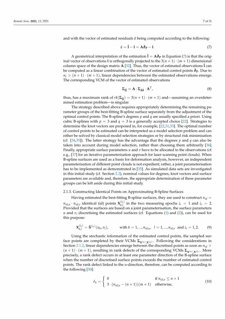
Using the stochastic information of the estimated control points, the sampled sur-face points are completed by their VCMs ΣX(ie),X(ie) . Following the considerations inSection 2.1.2, linear dependencies emerge between the discretised points as soon as nid >(n + 1) · (m + 1), resulting in rank defects of the corresponding VCMs ΣX(ie),X(ie) . Moreprecisely, a rank defect occurs in at least one parameter direction of the B-spline surfacewhen the number of discretised surface points exceeds the number of estimated controlpoints. The rank defect linked to the u-direction, therefore, can be computed according tothe following [30]:

δu =

0 if nid,u ≤ n + 1

3 · (nid,u − (n + 1))(m + 1) otherwise,(10)

Remote Sens. 2021, 13, 3551 8 of 31

and the rank defect linked to the v-direction accordingly arises to the following:

δv =

0 if nid,v ≤ m + 1

3 · (nid,v − (m + 1))(n + 1) otherwise.(11)

The overall rank defect δ is the sum of these two parts [30]:

δ = δu + δv. (12)

This singularity in the VCMs of the corresponding points represents an important dif-ference to deformation models in which the observed data points are directly incorporated.

2.1.4. Estimation of Rigid Body Movements

The estimation of rigid body movements of an object of interest is based on nid three-dimensional corresponding points X(1)

k,l and X(2)k,l (k = 1, . . . , nid,u, l = 1, . . . , nid,v) in two

measuring epochs, in this study on corresponding surface points (cf. Equation (9)).Assuming that the object undergoes solely rigid body movements, all corresponding

points—just like the entire surface—are subject to translations (summarised in the transla-tion vector t) and rotations (fully described by means of the rotation matrix R, containingthe rotation angles ω, φ and κ). Sometimes, a change of scale (indicated by the scale factor s)is also included, resulting in the mathematical formulation of a three-dimensional similaritytransform [1]:

X(2)k,l = s · R · X(1)

k,l + t, k = 1, . . . , nid,u, l = 1, . . . , nid,v. (13)

When estimating the parameters of the similarity transform t, R and s based onthe corresponding surface points, it must be taken into account that both the points X(1)

k,l

available in the start system and the points X(2)k,l available in the target system are defined

by estimated B-spline surfaces and, thus, are subject to uncertainties. In order to includethe stochastic information of both point groups into the estimation of the transformationparameters, two strategies, delivering identical results, exist [38]: Either the transformationparameters are estimated in a Gauß–Helmert model, or the classical Gauß–Markov model,assuming the points in the start system to be deterministic, is extended. Because of theeasier possibility to extend the approach to a robust one, the second variant is chosenhere [30].

Assuming that the data sets under investigation are acquired by means of the samelaser scanner and, hence, neglecting the scale factor s, the extended functional model toestimate the transformation parameters is then given by the following [38]:

X(2)k,l = X(2)

k,l + e(2)k,l = R · X∗(1)k,l + t (14)

X(1)k,l = X(1)

k,l + e(1)k,l = X∗(1)k,l , (15)

with e(ie)k,l (ie = 1, 2) being residual vectors. The first part of the model (Equation (14))describes the functional relationship between the identical points in the two epochs bymeans of the unknown transformation parameters. Equation (15) simultaneously intro-duces the coordinates of the identical points in the start system as additional observationsand, thus, allows for the consideration of their stochastic information. The link betweenEquations (14) and (15) is given by the estimated point coordinates available in the startsystem, which are introduced in both equations and are marked with an asterisk. Neglect-

Remote Sens. 2021, 13, 3551 9 of 31

ing inter-epochal correlations, the extended stochastic model is composed of the VCMsΣX(1)X(1) as well as ΣX(2)X(2) of the constructed surface points, resulting in the following [38]:

Σll =

[ΣX(2)X(2) 0

0 ΣX(1)X(1)

]= σ2

0 ·Qll. (16)

Based on the functional model in Equations (14) and (15) as well as on the stochasticmodel in Equation (16), the unknown transformation parameters can be estimated in anon-linear Gauß–Markov model (cf. [38] for more information).

2.1.5. Robust Estimation of Rigid Body Movements

The derivations in Section 2.1.4 are based on the assumption that the object underinvestigation is only subject to rigid body movements. However, rigid body movementsare usually superimposed by additional distortions in reality. When taking into accountpoints that are subject to both rigid body movements and distortions in the estimation ofthe rigid body movement, these points falsify the estimated transformation parameters.As a consequence, the determination of transformation parameters must necessarily beaccompanied by an elimination of surface points in distorted areas. Otherwise, the requiredcongruence of identical points is not given.

Considering points that are subject to both rigid body movements and distortion tobe outliers in the context of the similarity transform is one possible strategy to cope withthis challenge [30]. In order to accurately estimate rigid body movements in this situation,a robust strategy based on the random sample consensus (RANSAC)-algorithm [39] isproposed in this section. In general, RANSAC is an easy-to-implement method and is char-acterised by a high breakpoint (>50%). Furthermore, with respect to the presented problem,RANSAC allows for the robust estimation of rigid body movements while obtaining initialinformation about non-distorted regions.

The general idea of RANSAC is to initially determine the unknown parameters of amodel describing nl data points by the minimum number nsub of data points that is neededfor this determination [39]. These nsub data points are randomly drawn from the entireset of data points. After having computed the model parameters by means of these nsubpoints, the distances of the resulting preliminary model to the entirety of the data pointsare calculated. Points with distances that are within a predefined error tolerance ε areconsidered to be consistent with the determined model parameters. These points form theconsensus set SCS. The procedure is repeated iteratively until either the number of pointsin the consensus set equals a specified minimum number nmin or a maximum number ofiterations imax is performed. Finally, the points in the largest consensus set are used toestimate the optimal model parameters.

RANSAC can be directly applied to the robust estimation of rigid body movementsthat are superimposed by distortions (see Figure 4 for a schematic sketch of the proce-dure): the six parameters of a three-dimensional similarity transform with neglected scalefactor (cf. Equation (14)) can principally be determined by means of two pairs of three-dimensional corresponding data points. However, the estimation of the transformationparameters described in Section 2.1.4 is a non-linear estimation problem and, thus, requiresapproximate values. As these approximate values are determined by means of quaternions(see, for example, [40]) in this study, a strategy that also yields the scale factor s, the numberof point pairs required is nsub = 3. Hence, three pairs of sampled surface points are re-peatedly and randomly drawn from the entirety of surface points and are afterwards usedto determine approximate parameters t0, R0 and s0 by means of a quaternion approach.(Strictly speaking, the modelled transformation is not a rigid body movement in this step.However, as the results are only approximate values for the final estimation of rigid bodymovements, this strategy is not to be regarded as critical.) Unlike the quaternion approach,the strategy presented in Section 2.1.4 allows for the accuracies of the corresponding pointsto be taken into account when estimating rigid body movements. For this reason, the ap-proximate parameters are improved in a second step as described above, yielding optimal

Remote Sens. 2021, 13, 3551 10 of 31

translations t0 and optimal rotations R0, describing the rigid body movements of the threechosen surface points. During this step, the scale factor is set to s = 1 [30]. The entirety ofcomputed surface points of the first measuring epoch X(1)

k,l is afterwards transformed usingthe estimated transformation parameters as follows:

X(1)tr,k,l = R0 · X(1)

k,l + t0, k = 1, . . . , nid,u l = 1, . . . , nid,v. (17)

Start

Random selection of nsub pairsof corresponding points

Determination of approximatevalues t0, R0 and s0 using quaternions

Estimation of t0 and R0 (s = 1)based on the nsub point pairs

Transforming X(1)

using t0 and R0 yields X(1)tr

Computation of distances dk,l (incl. σdk,l)

between X(2)k,l and X

(1)tr,k,l

Building SCS with nCS point pairsfulfilling dk,l ≤ εk,l = τ · σdk,l

nCS ≥ nmini ≥ imax

Final estimation oftCS and RCS

using SCS

Final estimation oftCS and RCS

using SCS withmaximum nCS

Global test:TG < Ff,∞

End

i = 1

no

yes

no

i = i + 1

yes

no

yes

Figure 4. Flow chart of the RANSAC-based estimation of rigid body movements [30].

The Euclidean distance

dk,l = ||X(1)tr,k,l − X(2)

k,l || (18)

between each transformed point X(1)tr,k,l belonging to epoch E1 and its corresponding point

X(2)k,l belonging to epoch E2 provides the basis for the decision of whether a surface point is

Remote Sens. 2021, 13, 3551 11 of 31

included in the consensus set of model-conforming points. This distance is compared tothe error tolerance as follows:

εk,l = τ · σdk,l(19)

which is determined by the accuracy σdk,lof the computed distance dk,l , arising from vari-

ance covariance propagation as well as a factor τ, which needs to be chosen appropriately(see below). According to Equation (19), the error tolerance is assessed for each point pairindividually since the discretised surface points are not available with a homogeneousprecision [30]. When

dk,l ≤ εk,l (20)

is fulfilled, the corresponding point pair is assigned to the consensus set SCS.This procedure is repeated either until the number nCS of points fulfilling Equation (20)

is larger than or equal the minimum size nmin of the consensus set or until the maximumnumber of iterations imax is reached. It is worth noting that it is not possible to distinguishdistortions from gross errors in the data during this step. For this reason, it is essential tosuccessfully remove gross errors a priori using standard techniques, for example, whenestimating best-fitting B-spline surfaces.

The successful application of the developed strategy requires the definition ofthree parameters:

• The parameter τ in Equation (19) has to be chosen in such a way that only model-compliant points are included in SCS. When τ is chosen too small, points will beerroneously identified as outliers, whereas when τ is chosen too large, outliers maybe included in the consensus set and, thus, the estimation result will become biased.The influence of the parameter τ on the results is investigated in Section 3.2.

• The minimum number nmin of model-compliant points required to accept the currentSCS is estimated from the expected amount of gross errors nerr (0 ≤ nerr ≤ 1) containedin the data set. When nerr is known, the optimal nmin can be determined accordingto the following [41]:

nmin = (1− nerr) · nid. (21)

• The maximum number of iterations imax is determined by the desired probability Pthat a solution without outliers is found [41]:

imax =log(1− P)

log(1− (1− nerr)nsub). (22)

Finally, after the iteration is completed, the point pairs of the largest consensus set areused to estimate the transformation parameters tCS and RCS in the extended Gauß–Markovmodel (14) and (15).

With a final statistical global test, comparing the respective a priori variance factorσ2

0 with the corresponding a posteriori variance factor σ20 , the presence of outliers can be

excluded with a confidence probability of 1− αG, with αG being the error probability [42]:

Null hypothesis H0,G : Eσ20 = σ2

0 (23)

Alternative hypothesis HA,G : Eσ20>σ2

0 . (24)

The corresponding test variable TG is F-distributed with the degrees of freedom f and ∞:

TG =σ2

0σ2

0∼ Ff ,∞. (25)

Remote Sens. 2021, 13, 3551 12 of 31

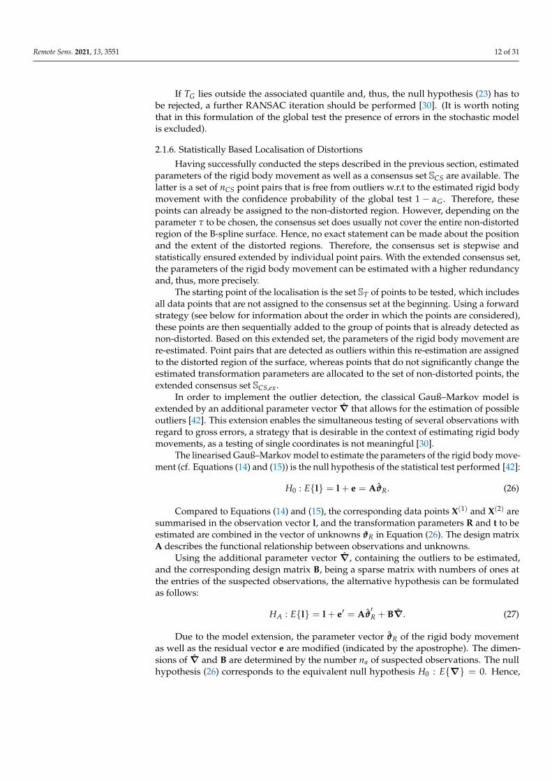
If TG lies outside the associated quantile and, thus, the null hypothesis (23) has tobe rejected, a further RANSAC iteration should be performed [30]. (It is worth notingthat in this formulation of the global test the presence of errors in the stochastic modelis excluded).

2.1.6. Statistically Based Localisation of Distortions

Having successfully conducted the steps described in the previous section, estimatedparameters of the rigid body movement as well as a consensus set SCS are available. Thelatter is a set of nCS point pairs that is free from outliers w.r.t to the estimated rigid bodymovement with the confidence probability of the global test 1 − αG. Therefore, thesepoints can already be assigned to the non-distorted region. However, depending on theparameter τ to be chosen, the consensus set does usually not cover the entire non-distortedregion of the B-spline surface. Hence, no exact statement can be made about the positionand the extent of the distorted regions. Therefore, the consensus set is stepwise andstatistically ensured extended by individual point pairs. With the extended consensus set,the parameters of the rigid body movement can be estimated with a higher redundancyand, thus, more precisely.

The starting point of the localisation is the set ST of points to be tested, which includesall data points that are not assigned to the consensus set at the beginning. Using a forwardstrategy (see below for information about the order in which the points are considered),these points are then sequentially added to the group of points that is already detected asnon-distorted. Based on this extended set, the parameters of the rigid body movement arere-estimated. Point pairs that are detected as outliers within this re-estimation are assignedto the distorted region of the surface, whereas points that do not significantly change theestimated transformation parameters are allocated to the set of non-distorted points, theextended consensus set SCS,ex.

In order to implement the outlier detection, the classical Gauß–Markov model isextended by an additional parameter vector ∇ that allows for the estimation of possibleoutliers [42]. This extension enables the simultaneous testing of several observations withregard to gross errors, a strategy that is desirable in the context of estimating rigid bodymovements, as a testing of single coordinates is not meaningful [30].

The linearised Gauß–Markov model to estimate the parameters of the rigid body move-ment (cf. Equations (14) and (15)) is the null hypothesis of the statistical test performed [42]:

H0 : El = l + e = AϑR. (26)

Compared to Equations (14) and (15), the corresponding data points X(1) and X(2) aresummarised in the observation vector l, and the transformation parameters R and t to beestimated are combined in the vector of unknowns ϑR in Equation (26). The design matrixA describes the functional relationship between observations and unknowns.

Using the additional parameter vector ∇, containing the outliers to be estimated,and the corresponding design matrix B, being a sparse matrix with numbers of ones atthe entries of the suspected observations, the alternative hypothesis can be formulatedas follows:

HA : El = l + e′ = Aϑ′R + B∇. (27)

Due to the model extension, the parameter vector ϑR of the rigid body movementas well as the residual vector e are modified (indicated by the apostrophe). The dimen-sions of ∇ and B are determined by the number na of suspected observations. The nullhypothesis (26) corresponds to the equivalent null hypothesis H0 : E∇ = 0. Hence,

Remote Sens. 2021, 13, 3551 13 of 31

it is examined whether the estimated gross errors differ significantly from zero. Thetest variable

T =∇T

Q−1∇∇∇

na · σ2′0

∼ Fna , f−na , (28)

used to investigate the validity of the null hypothesis, follows the F-distribution Fna , f−na ,the degrees of freedom of which are determined by the number na of suspected observationsas well as the redundancy f of the initial estimation problem [42]. The computation of Trequires the determination of the following quantities:

Qεε = Q−1ll −A(ATQ−1

ll A)−1A (29)

−ε = QεεQ−1ll l (30)

Q∇∇ = (BTQ−1ll QεεQ−1

ll B)−1 (31)

∇ = −Q∇∇BTQ−1ll ε (32)

Ω′ = εTQ−1ll ε− ∇T

Q−1∇∇∇ (33)

σ2′0 =

Ω′

f − na. (34)

In the equations above, Qεε is the cofactor matrix of the vector of residuals ε, Q∇∇the cofactor matrix of the additional parameter vector ∇ and Ω′ the corrected sum ofsquared residuals.

With the strategy described above, the stability of single point pairs X(1,2)k,l with respect

to distortions can be evaluated in a statistically ensured way (single point test).In order to obtain an areal character of the localisation, alternatively, a predefined

domain of the surface can be included in the outlier detection. A straightforward way todefine this domain is to use the parametric neighbourhood [uk−a, uk+a]× [vl−a, vl+a] of theinvestigated point pair X(1,2)

k,l = S(1,2)(uk, vl) (see Figure 5 for an example with a = 1). Theparameter a to be chosen determines the size of the neighbourhood. Depending on thechoice of a,

na = 3(2a + 1)2 (35)

observations are examined for gross errors [30]. Naturally, Equation (35) does only holdwhen X(1,2)

k,l does not lie at the surface’s boundary. In that case, na reduces accordingly.

Investigated point

∈ SCS

6∈ SCS

Considered in testing

uk−2 uk−1 uk uk+1 uk+2

vl+2

vl+1

vl

vl−1

vl−2

Figure 5. Schematic sketch of the domain that is considered in the outlier detection. The domain ispredefined by the neighbourhood [uk−1, uk+1]× [vl−1, vl+1] (a = 1) of the surface point S(uk, vl) [30].

Remote Sens. 2021, 13, 3551 14 of 31

Having determined the neighbourhood of the point pair to be tested, all point pairslying in the domain [uk−a, uk+a]× [vl−a, vl+a] are temporarily included in the extendedconsensus set SCS,ex by adjusting the matrix B (cf. Equation (24)) accordingly. (It is worthnoting that previous test decisions on neighbouring points are not taken into account duringthis step: neighbouring points that have already been allocated either to the distorted orto the non-distorted regions as well as points that have not been under investigation yetare equally treated and, thus, are involved in the formation of the neighbourhood.) If thecomparison of the resulting test variable Tk,l (cf. Equation (28)) with the correspondingquantile of the Fisher distribution supports the null hypothesis, the existence of gross errorscan be ruled out with the respective confidence probability 1− α. As a consequence, thepoint pair under investigation is added to the extended consensus set and is considerednon-distorted in the subsequent outlier tests. Otherwise, if the null hypothesis has tobe rejected, a distortion of the surface in the domain that is under investigation must beassumed. In this case, the extended consensus set is not modified. With the removal ofthe point pair X(1,2)

k,l from ST , an iteration step of the procedure is completed and the nextpoint pair is investigated. The procedure is continued until all point pairs are removedfrom ST . At the end, the extended consensus set is used to estimate the final parameters ofthe rigid body movement. Additionally, a completing global test can be used to check theconsistency of the detected non-distorted point pairs.

The order in which the point pairs are investigated by means of the strategy describedabove, is determined by their degree of consistency with the determined rigid body move-ment. For this purpose, all points X(1)

k,l to be tested are transformed using the transformationparameters RCS,ex and tCS,ex, determined by means of the (extended) consensus set. The

transformed points X(1)tr,k,l are then compared with their correspondences X(2)

k,l by computingthe Euclidean distances dk,l (cf. Equation (18)). Since a small dk,l indicates the consensusof the corresponding point pair with the estimated transformation model, of all the pointpairs to be tested, the one with the smallest dk,l is examined first [30]. The strategy tolocalise the distortions is summarised in the schematic sketch in Figure 6.

2.1.7. Regularisation of the System of Equations

By taking into account the accuracies of the sampled surface points, the system ofequations for estimating the transformation parameters becomes singular as soon as moresurface points are sampled than control points have been estimated (cf. Section 2.1.3). How-ever, in order to achieve a (quasi)-continuous statement regarding the position and extentof the distortions, the number of sampled surface points should considerably exceed thenumber of control points [30]. The associated singularities of the system of equations mustbe taken into account accordingly. In [30], three possibilities to deal with the singularities—neglecting the correlations between the estimated surface points, use of the pseudoinverseand regularisation of the VCM’s main diagonal—are investigated and compared. As thesecond strategy outperforms the first and the third one w.r.t the correctness of the resultsachieved, the pseudoinverse is used in this contribution if not stated otherwise.

2.2. Data Sets under Investigation2.2.1. Data Simulation

The B-spline-based strategy to estimate rigid body movements and to simultaneouslydetect non-distorted regions introduced in Section 2.1 is applied to a variety of simulateddata sets in this study, the simulation process of which is demonstrated by means of anexample data set. Due to the use of simulated data, the obtained results can be comparedwith nominal surfaces and nominal transformation parameters and, thus, the developedstrategy can be directly validated.

The starting point of the data simulation is the cubic B-spline surface with (n + 1) ·(m + 1) = 7 · 9 = 63 control points presented in Figure 7. This surface is considered thereference surface in the remainder of this section.

Remote Sens. 2021, 13, 3551 15 of 31

Establishment of ST

Estimation of RCS,ex

and tCS,ex using SCS,ex

ST = End

Determination of X(1)tr by transforming

X(1) with RCS,ex and tCS,ex

Computation of distances between X(1)tr

and their correspondences X(2)

Selection of the point pair X(1,2)k,l ,

with minimal distance

Determination of the neighbourhood[uk−a, uk+a]× [vl−a, vl+a]

Computation of the test variable Tk,l

and the corresponding quantile Fk,l,

removal of X(1,2)k,l from ST

Tk,l ≤ Fk,l

Allocation of X(1,2)k,l to SCS,ex

yes

no

yes

no

Figure 6. Flow chart of the localisation of distorted regions [30].

The scanning process of this object during the first measuring epoch E1 is emu-lated by regularly sampling the B-spline surface along the parameter lines, resulting in10,000 surface points with a spatial resolution of 4–5 mm. Afterwards, the surface points aresuperimposed by normally distributed measuring noise n ∼ N (0, Σnn), with Σnn beingthe VCM of the measuring noise. In these initial studies, the measuring noise is modelledto be uncorrelated, with a standard deviation of σnx = σny = σnz =

13 mm. The choice of

these specific values characterising the data points’ precision leads to an average pointerror of 1 mm [30].

In order to simulate the point cloud of the second epoch E2, the reference surfaceis distorted by moving one or more control points. This approach exploits the localityof B-spline surfaces (cf. Section 2.1.1), meaning that the movement of a single controlpoint changes only a local part of the surface. For example, moving control point P3,3 (redtriangle in Figure 7) by 1.2 cm upwards results in a maximum distortion of the B-splinesurface of up to 6 mm. Figure 8 presents the distances between corresponding points onthe reference surface and on the distorted surface in the parameter space (cf. Equation (1)for the relationship between Cartesian coordinates and surface parameters). As can beseen, only parts of the parameter space are influenced by the control point’s movement (thenon-distorted parts are not coloured). In most of the distorted area, the distances between

Remote Sens. 2021, 13, 3551 16 of 31

corresponding surface points are very small (<1 mm, coloured in green). Compared tothe simulated measurement noise, these deviations w.r.t to the reference surface are notsignificant. The largest deformation occurs in the middle of the distorted part (coloured inred), with a maximum distortion of up to 6 mm.

Figure 7. Reference surface and corresponding control points (triangles) used for the datasimulation [30]. Red triangle: control point P3,3. The X-axis complements the right-handed co-ordinate system, and the surface’s colouring gives an idea of its height in the X direction.

Figure 8. Distances d between corresponding surface points after having shifted control point P3,3 by1.2 cm in x-direction. Presentation of the influenced area in the parameter space [30].

Remote Sens. 2021, 13, 3551 17 of 31

Afterwards, the distorted B-spline surface is subjected to a similarity transform withneglected scale factor, using the B-splines’ property of invariance w.r.t a similarity transform.For all generated data sets, the following transformations and rotations are chosen:

tT =[

0.300 m 0.600 m 0.000 m]

(36)[ω φ κ

]T=[

35.000 gon 0.000 gon −10.000 gon]T (37)

The control points of the distorted and transformed B-spline surface, therefore, resultfrom the following:

P(2)ij = R · P(1)∗

ij + t, (38)

with the asterisk indicating the local distortion w.r.t the reference surface.Finally, a noisy point cloud consisting of 10,000 data points is created by sampling the

distorted and transformed B-spline surface and by subsequently adding white noise asdescribed above.

The results of the data simulation are two noisy point clouds describing an objectin two measuring epochs that is subject to rigid body movements and superimposedlocal distortions.

2.2.2. Introduction of the Simulated Data Sets

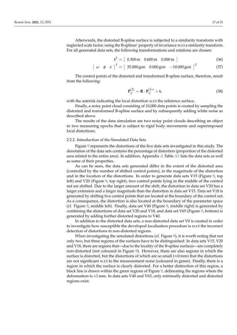
Figure 9 represents the distortions of the five data sets investigated in this study. Thedenotation of the data sets contains the percentage of distortion (proportion of the distortedarea related to the entire area). In addition, Appendix A Table A1 lists the data sets as wellas some of their properties.

As can be seen, the data sets generated differ in the extent of the distorted area(controlled by the number of shifted control points), in the magnitude of the distortionand in the location of the distortions. In order to generate data sets V15 (Figure 9, topleft) and V20 (Figure 9, top right), two control points lying in the middle of the controlnet are shifted. Due to the larger amount of the shift, the distortion in data set V20 has alarger extension and a larger magnitude than the distortion in data set V15. Data set V18 isgenerated by shifting five control points that are located at the boundary of the control net.As a consequence, the distortion is also located at the boundary of the parameter space(cf. Figure 9, middle left). Finally, data set V40 (Figure 9, middle right) is generated bycombining the distortions of data set V20 and V18, and data set V65 (Figure 9, bottom) isgenerated by adding further distorted regions to V40.

In addition to the distorted data sets, a non-distorted data set V0 is created in orderto investigate how susceptible the developed localisation procedure is w.r.t the incorrectdetection of distortions in non-distorted regions.

When investigating the simulated distortions (cf. Figure 9), it is worth noting that notonly two, but three regions of the surfaces have to be distinguished: In data sets V15, V20and V18, there are regions that—due to the locality of the B-spline surfaces—are completelynon-distorted (not coloured in Figure 9). However, there are also regions in which thesurface is distorted, but the distortions of which are so small (≈0 mm) that the distortionsare not significant w.r.t to the measurement noise (coloured in green). Finally, there is aregion in which the surface is clearly distorted. For a better distinction of this region, ablack line is drawn within the green regions of Figure 9, delineating the regions where thedeformation is >1 mm. In data sets V40 and V65, only minimally distorted and distortedregions exist.

Remote Sens. 2021, 13, 3551 18 of 31

Figure 9. Simulated distortions, presented in the parameter space. The knot grid is indicated by the grey lines. Top left: V15;top right: V20; middle left: V18; middle right: V40; bottom: V65 [30].

Remote Sens. 2021, 13, 3551 19 of 31

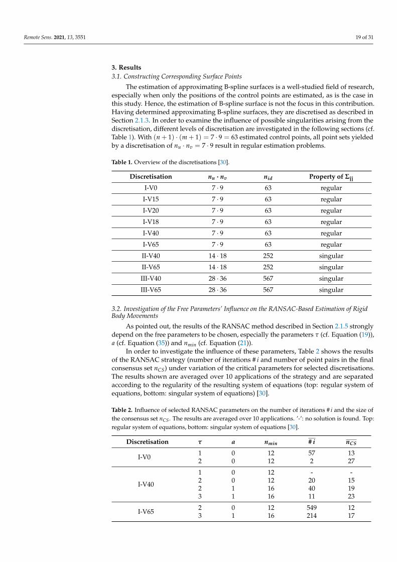
3. Results3.1. Constructing Corresponding Surface Points

The estimation of approximating B-spline surfaces is a well-studied field of research,especially when only the positions of the control points are estimated, as is the case inthis study. Hence, the estimation of B-spline surface is not the focus in this contribution.Having determined approximating B-spline surfaces, they are discretised as described inSection 2.1.3. In order to examine the influence of possible singularities arising from thediscretisation, different levels of discretisation are investigated in the following sections (cf.Table 1). With (n + 1) · (m + 1) = 7 · 9 = 63 estimated control points, all point sets yieldedby a discretisation of nu · nv = 7 · 9 result in regular estimation problems.

Table 1. Overview of the discretisations [30].

Discretisation nu · nv nid Property of Σll

I-V0 7 · 9 63 regular

I-V15 7 · 9 63 regular

I-V20 7 · 9 63 regular

I-V18 7 · 9 63 regular

I-V40 7 · 9 63 regular

I-V65 7 · 9 63 regular

II-V40 14 · 18 252 singular

II-V65 14 · 18 252 singular

III-V40 28 · 36 567 singular

III-V65 28 · 36 567 singular

3.2. Investigation of the Free Parameters’ Influence on the RANSAC-Based Estimation of RigidBody Movements

As pointed out, the results of the RANSAC method described in Section 2.1.5 stronglydepend on the free parameters to be chosen, especially the parameters τ (cf. Equation (19)),a (cf. Equation (35)) and nmin (cf. Equation (21)).

In order to investigate the influence of these parameters, Table 2 shows the resultsof the RANSAC strategy (number of iterations # i and number of point pairs in the finalconsensus set nCS) under variation of the critical parameters for selected discretisations.The results shown are averaged over 10 applications of the strategy and are separatedaccording to the regularity of the resulting system of equations (top: regular system ofequations, bottom: singular system of equations) [30].

Table 2. Influence of selected RANSAC parameters on the number of iterations # i and the size ofthe consensus set nCS. The results are averaged over 10 applications. ’-’: no solution is found. Top:regular system of equations, bottom: singular system of equations [30].

Discretisation τ a nmin # i nCS

I-V0 1 0 12 57 132 0 12 2 27

I-V40

1 0 12 - -2 0 12 20 152 1 16 40 193 1 16 11 23

I-V65 2 0 12 549 123 1 16 214 17

Remote Sens. 2021, 13, 3551 20 of 31

Table 2. Cont.

Discretisation τ a nmin # i nCS

II-V40

2 0 12 37 312 1 40 316 463 0 16 220 373 1 30 684 44

II-V652 0 12 86 202 1 20 810 233 1 16 1495 28

III-V40

2 0 12 310 182 1 16 1015 323 0 12 - -

III-V65

2 0 12 892 163 0 12 - -

The choice of τ = 1 is investigated for the undistorted data set I-V0 as well as fordata set I-V40. Both applications reveal that this choice is too pessimistic: Although a verysmall consensus set can be found after relatively many iterations for I-V0, no solution isfound even after hundreds of iterations for I-V40. When using τ = 2 in combination with aregular system of equations, the error threshold (19) is increased and, as a consequence,the number of required iterations is clearly reduced both for data set I-V0 and I-V40. Thechoice of τ = 2 also results in a sufficiently large consensus set for data set I-V65, butrequires a very large number of iterations. The further increase to τ = 3 leads to a furtherreduction of the iterations and a larger consensus set. Values of τ > 3 are not considered atthis point: taking into account the 3-σ-rule (cf. [1]), it must be expected that these choicesare not realistic.

An opposite behaviour is apparent when considering the data sets causing a singularsystem of equations: The increase from τ = 2 to τ = 3 leads to a significant increase ofthe required iterations for almost all examined data sets. Although the pure RANSACprocedure converges after a decreased number of iterations, the resulting consensus setsdo not pass the final global test, making further iteration steps necessary. This effectis intensified by a reduced level of discretisation as well as by an increasing amount ofdistortions. As a consequence, the use of τ = 3 does not at all result in a consensusset for which the final global test is successful when considering data sets III-V40 andIII-V65. Furthermore, it is noticeable that—although the overall number of points increasessignificantly by increasing the discretisation density—the size of the consensus set does not.

When a and, thus, the size of the neighbourhood considered in the outlier test areincreased, the minimum size nmin of the consensus set changes [30]. This behaviour is dueto the fact that the maximum number of observations that can be included in the outlier testis influenced by the redundancy of the initial model [42]. Because of the increase of nmin,the number of required iterations and the size of the resulting consensus set also increase.

The investigations reveal that a threshold determination with τ = 2 and τ = 3 deliversa sufficiently large consensus set for the subsequent deformation analysis when consideringa discretisation with a 7 · 9 grid. With τ = 3 both a reduction of the required iterations andan enlargement of the final consensus set can be achieved [30]. However, falsifications ofthe consensus set due to point pairs lying in the slightly deformed area are to be expectedmore frequently for τ = 3. As the subsequent global test rules out the existence of thesegross errors with a confidence probability of 1− αG, nevertheless, τ = 3 will be used in thefollowing investigations when considering a regular system of equations. However, theuse of τ = 3 is not expedient when considering an increased discretisation density. Hence,τ = 2 is used in these cases.

Remote Sens. 2021, 13, 3551 21 of 31

Finally, it is worth noting that not only the parameters of the RANSAC algorithminfluence the results of the deformation analysis, but also the choice of the significancelevels 1-α and 1-αG: the larger the significance level, the smaller the probability of type Ierrors, whereas the probability of type II errors can be reduced by appropriately decreasingthe significance level. Despite this relationship, the significance levels are not consideredtuning constants in this contribution as these parameters are usually fixed or chosen w.r.tthe hazard that is monitored.

3.3. Deformation Analysis with a Regular System of Equations

Six discretisations listed in Table 1 (I-V0, . . . , I-V65) result in a regular system ofequations. These data sets are used in this section to demonstrate the general applicabilityof the developed strategy.

3.3.1. Deformation Analysis for Data Set V0 (No Distortions)

Applying the RANSAC-based estimation of the rigid body movements to the undis-torted data set V0 results in the estimated transformation parameters listed in Table 3.Obviously, the rigid body movement can be estimated very accurately and very preciselyfor data sets without an additional distortion.

When applying the localisation strategy to data set V0, the majority of point pairs iscorrectly determined to be non-distorted, but also a few type I errors occur. Table 4 liststhe testing results for selected point pairs of data set V0 in dependence of the parameter a,specifying the neighbourhood used during the testing. In addition to the test variable T andthe corresponding 99%-quantile F99, the size nCS of the consensus set and the distance dbetween the respective point pair is given. Type I errors are printed bold. As shown by theexample X(1,2)

2,5 , a type I error can be eliminated by considering the direct neighbourhoodinstead of the single point during the test. However, the exact opposite happens in thecase of point X(1,2)

3,4 : being detected as non-distorted in the single point test, it is incorrectlydetermined as distorted when the direct neighbourhood is taken into account. Thus, theoccurrence of type I errors cannot be eliminated by defining a suitable neighbourhood.In any case, tests with a = 1 lead to a homogenisation of the calculated test variables [30].Remarkably, type I errors occur exclusively in the interior of the surface, whereas edge(e.g., X(1,2)

0,1 ) and corner points (e.g., X(1,2)6,8 ) are correctly detected to be non-distorted [30].

Table 3. Results of the estimated rigid body movement (data set V0) [30].

tx [m] 0.300 σtx [mm] 0.023

ty [m] 0.600 σty [mm] 0.015

tz [m] 0.000 σtz [mm] 0.026

ω [gon] 35.002 σω [mgon] 3.816

φ [gon] 0.008 σφ [mgon] 4.392

κ [gon] −9.997 σκ [mgon] 4.279

Remote Sens. 2021, 13, 3551 22 of 31

Table 4. Results of the localisation for selected point pairs (data set V0). Type I errors are printed inbold [30].

a d [mm] nCS T F99

X(1,2)0,1

0 0.206 26 1.17 4.081 0.206 20 1.63 2.36

X(1,2)2,5

0 0.180 54 4.82 3.911 0.180 47 1.23 1.90

X(1,2)3,4

0 0.111 26 1.08 4.081 0.111 21 2.23 2.13

X(1,2)6,8

0 0.717 62 3.48 3.891 0.717 56 1.62 2.30

3.3.2. Deformation Analysis of Data Sets V15 and V20 (Distortions in the Middle ofthe Surface)

Table 5 summarises the final results of the estimated rigid body movements for dataset V15 when using the single point test (a = 0). The initial consensus set of nCS is extendedduring the localisation procedure by 20 point pairs (nCS,ex = 45). The resulting estimatedparameters of the rigid body movement differ only minimally from those of the non-distorted data set V0 (cf. Table 3). Noticeable differences are only visible in the standarddeviations of the estimated parameters, which are slightly larger for data set V15 than fordata set V0. The effect is amplified when the direct neighbourhood is included in the tests(a = 1, Table 6). As the initial consensus set is validated by means of individual tests witha = 1 before performing the localisation (cf. Section 2.1.6), the validated consensus set issmaller than the initial consensus set for a = 0 (nCS,val = 14). A similar behaviour can beseen in the sizes of the extended consensus sets: When single point tests are performed,SCS,ex is clearly larger (nCS,ex = 45)—and, thus, the distorted region significantly smaller—than when the direct neighbourhood is considered during the testing (nCS,ex = 28). Thiseffect is also evident from Figure 10, presenting for all point pairs the computed test valuesT of the localisation procedure and the resulting test decision both for a = 0 (left) and fora = 1 (right). However, both scenarios (a = 0 and a = 1) have in common that, regardlessof the choice of the initial SCS, the null hypothesis (23) of the global test is accepted afterhaving extended the consensus set.

Table 5. Results of the estimated rigid body movement after having extended SCS (data set V15,a = 0, nCS = 25, nCS,ex = 45) [30].

tx [m] 0.300 σtx [mm] 0.026

ty [m] 0.600 σty [mm] 0.017

tz [m] 0.000 σtz [mm] 0.028

ω [gon] 35.000 σω [mgon] 4.211

φ [gon] 0.010 σφ [mgon] 4.912

κ [gon] −9.997 σκ [mgon] 4.848

Remote Sens. 2021, 13, 3551 23 of 31

Table 6. Results of the estimated rigid body movement after having extended SCS (data set V15,a = 1, nCS,val = 14, nCS,ex = 28) [30].

tx [m] 0.300 σtx [mm] 0.037

ty [m] 0.600 σty [mm] 0.027

tz [m] 0.000 σtz [mm] 0.045

ω [gon] 34.994 σω [mgon] 6.880

φ [gon] 0.000 σφ [mgon] 9.491

κ [gon] −10.008 σκ [mgon] 7.951

The estimated transformation parameters achieved by means of data set V20 (analo-gously to V15 summarised in the Appendix B Tables A2 and A3) are almost identical tothose yielded by data set V15. The distortions’ dimension and/or magnitude, however,seem to have an influence on the standard deviations of the estimated parameters, as theyare larger for data set V20 than for data set V15. Moreover, when using single point testsfor data set V20 (Table A2), an unexpected behaviour can be observed: although everynull hypothesis of the localisation procedure (26) for point pairs added to the extendedconsensus set is accepted, the null hypothesis (23) of the final global test has to be rejected.When changing the initial consensus set, it can further be observed that this behaviour doesnot always occur, but seems to strongly depend on the choice of the initial consensus set.A detailed investigation reveals that point pairs in the transition area between distortedand non-distorted regions are the reason for this behaviour: when those point pairs areassigned to the initial consensus set, the null hypothesis of the global test has to be rejected,whereas it is accepted when only point pairs clearly lying in the non-distorted region arecontained in the initial consensus set. Furthermore, it can be observed that increasing thesize of the initial consensus set also leads to an increased success of the final global test.

Figure 10. Test values T of the localisation procedure for data set V15. For the circled points, the null hypothesis has to berejected and, hence, these points are assumed to lie in the distorted region. Left: a = 0, right: a = 1.

3.3.3. Deformation Analysis of Data Set V18 (Distortions at the Boundary of the Surface)

The results of the deformation analysis of data set V18 fully support the results ofV15 and V20: the transformation parameters can be estimated very accurately and veryprecisely (cf. Appendix B Tables A4 and A5), and the distortions can also be successfullydetected. When using the direct neighbourhood in the localisation procedure, the region

Remote Sens. 2021, 13, 3551 24 of 31

that is detected to be distorted is considerably larger than when single point tests areperformed (cf. Figure 11).

Figure 11. Test values T of the localisation procedure for data set V18. For the circled points, the null hypothesis has to berejected and, thus, these points are assumed to lie in the distorted region. Left: a = 0, right: a = 1.

3.3.4. Deformation Analysis of Data Sets V40 and V65 (Distortions in the Middle and at theBoundary of the Surface)

As for the data sets considered above, the estimated parameters of the rigid bodymovement (cf. Table 7 for a = 0 and Table 8 for a = 1) are very close to the nominal valuesfor data set V40.

Table 7. Results of the estimated rigid body movement after having extended SCS (data set V40,a = 0, nCS = 19, nCS,ex = 28) [30].

tx [m] 0.300 σtx [mm] 0.041

ty [m] 0.600 σty [mm] 0.028

tz [m] 0.000 σtz [mm] 0.045

ω [gon] 35.007 σω [mgon] 5.785

φ [gon] -0.004 σφ [mgon] 8.032

κ [gon] −10.025 σκ [mgon] 6.860

Table 8. Results of the estimated rigid body movement after having extended SCS (data set V40,a = 1, nCS,val = 7, nCS,ex = 7) [30].

tx [m] 0.300 σtx [mm] 0.141

ty [m] 0.600 σty [mm] 0.097

tz [m] 0.000 σtz [mm] 0.118

ω [gon] 35.014 σω [mgon] 12.867

φ [gon] -0.014 σφ [mgon] 20.105

κ [gon] −9.989 σκ [mgon] 21.812

However, the precision of the estimated parameters decreases further, both for thesingle point test and when considering the direct neighbourhood during the testing. Again,

Remote Sens. 2021, 13, 3551 25 of 31

the region detected as distorted becomes clearly larger when the direct neighbourhoodis considered than when a single point test is performed (cf. Appendix B Figure A1). Asfor data set V20, a dependency of the initial consensus set’s choice on the results can alsobe seen for data set V40: point pairs lying in the transition area between distorted andnon-distorted region of the surface are sometimes assigned to the distorted region andsometimes to the non-distorted region when the points in the initial consensus set arevaried. As a consequence, the null hypothesis of the final global test has to be rejected inthe latter case. Again, this behaviour can be reduced by increasing the size of the initialconsensus set.

Due to the large amount of distortions, only investigations with a = 0 are possible fordata set V65. The further increase in the amount of distortions compared to the previouslyinvestigated data sets results again in a rejection of the null hypothesis of the final globaltest. However, due to the small non-distorted regions, it is not possible to control the successof this data set’s deformation analysis by increasing the size of the initial consensus set.

3.4. Deformation Analysis with a Singular System of Equations

Using data set III-V40 as an example, the results of a deformation analysis with asingular system of equations are shortly presented in this section. Figure 12 (left) showsthe results of the localisation procedure for data set III-V40 when performing a single pointtest. Comparing this result to Figure A1 (left), presenting the equivalent result for I-V40,the large amount of type II errors lying in the transition zone between the two distortedregions is striking. However, as already described above, the number of type II errorscan be clearly reduced when the size nCS of the consensus set is increased. This effect isclearly visible in Figure 12 (right), showing the results of the localisation procedure whenthe consensus set is larger than in Figure 12 (left). Obviously, the separation of the twodistorted regions succeeds much more satisfactorily with the larger consensus set.

Figure 12. Test values T of the localisation procedure for data set III-V40 (a = 0, α = 5%). For the circled points, the nullhypothesis has to be rejected and, hence, these points are assumed to lie in the distorted region. Left: nCS = 14, right:nCS = 25.

4. Discussion

The developed strategy to estimate rigid body movements and simultaneously detectdistorted regions is applied to a variety of synthetic data sets, the distortions of whichvary in dimension and shape. The results presented in Section 3 reveal that—for justifiedselected free parameters of the algorithm—the estimated parameters of the rigid bodymovement are very close to the nominal values for all investigated data sets. Naturally,the larger the distorted region, the smaller the precision of the estimated parameters: due

Remote Sens. 2021, 13, 3551 26 of 31

to the reduced number of point pairs in the non-distorted region, the redundancy and,consequently, the precision of the estimated parameters decrease.

The localisation of the distorted areas on the basis of the data set V0 reveals that theoccurrence of type I errors cannot be completely avoided. However, since type I errorsusually do not occur in groups, most of them can be detected by investigating their directneighbourhoods: if their entire neighbourhood is located in the non-distorted region, itcan be assumed that a type I error exists. Furthermore, with a large confidence probability1− α, the probability of the occurrence of type I errors can be regulated.

The results of the data sets that indeed represent distorted objects show that clearlydistorted regions can be successfully detected in all investigated scenarios, independentlyof their location on the object. The only difficulty is to precisely distinguish the actualdistorted regions from the non-distorted ones. Particularly in the minimally distortedregions—usually, the transition region between distorted and non-distorted regions—,type II errors occur when performing single points tests: Point pairs lying in the minimallydistorted region are erroneously allocated to the non-distorted region. As a consequence,the final global test (αG = 5%) fails. This failure of the final global test can be reduced byconsidering the direct neighbourhood during the localisation procedure (a = 1) rather thanconducting single point tests (a = 0). Using this strategy, the minimally distorted regioncan be more successfully detected.

Hence, the success of the deformation analysis depends on a suitable choice of thefree parameters: Satisfactory results are obtained with a = 1 for scenarios with relativelylarge non-distorted regions (e.g., V15, V20 and V18), as is obvious when comparing thedetected distorted regions with the nominal ones. For data set V18 (results: Figure 11 (right),nominal: Figure 9 (middle left)), the non-distorted region is almost perfectly delimited fromthe distorted one. Only the discretised point S(1.00, 0.63) actually belongs to the distortedregion, but is assigned to the non-distorted region. However, as the actual distortion in thispoint is almost zero, the impact of this erroneous allocation is minimal. Similar results areachieved for data set V15 (results: Figure 10 (right), nominal: Figure 9 (top right)). Here,even seven points are erroneously allocated to the non-distorted region, all of them lyingon the surface’s boundary. However, the points’ positions are not the reason for the wrongallocation, but the minimal magnitude of the distortion.

The investigations using data sets V40 and V65 show that it is possible to satisfactorilyestimate rigid body movements, even when there are no non-distorted regions at all. Alter-natively, there must be regions in which the distortions are so small that they neverthelessare allocated to the consensus set. This behaviour can be observed particularly well bymeans of data set V40 (results: Figure A1 (right), nominal: Figure 9 (middle right)): Asfor data sets V18 and V15, few discretised points that are only minimally distorted areerroneously allocated to the non-distorted region. Nevertheless, the estimated parametersof the rigid body movement are very close to the nominal parameters. However, the largerthe distorted regions are, the more emphasis has to be placed on the definition of the initialconsensus set. The larger this consensus set is, the more reliably type II errors can beavoided, as the initial estimation of the rigid body movement succeeds more accurately.

Furthermore, the results of data set V40 show that also for data sets with large dis-torted regions, more accurate localisation results are achieved when considering the directneighbourhood during the localisation (a = 1) than when conducting single point tests(a = 0). However, for data sets in which the distorted regions occupy the majority of thesurface (data set V65), a localisation with a = 1 is no longer possible, and single point testsare the only option. In this case, the behaviour of single point tests that points that lie in theminimally distorted region are increasingly detected as non-distorted must be accepted. Totake advantage of the localisation using a = 1, it has to be ensured during data acquisitionthat a sufficiently large non-distorted area of the objects is captured.

Singularities arising from a decreased discretisation level can be successfully handledby using the pseudoinverse in all subsequent analysis steps. This approach allows to signifi-cantly increase the resolution of the results and, thus, to detect even small-scale distortions.

Remote Sens. 2021, 13, 3551 27 of 31

5. Conclusions

In this contribution, a strategy is introduced that allows for the estimation of rigid bodymovements of an object and for the simultaneous detection of distorted regions based onlaser scanning data. The starting points of the developed strategy are best-fitting B-splinesurfaces that approximate the point clouds acquired in at least two measuring epochs.Using the surface parameters u and v, point correspondences on these B-spline surfacesare defined. Based on these point correspondences, rigid body movements between thesurfaces are estimated. When the rigid body movements are superimposed by a localdistortion, the estimated parameters are falsified. In order to detect these gross errorsw.r.t to the rigid body movement, a robust RANSAC-based strategy to estimate rigid bodymovements is implemented. The result of this step is an initial solution for the rigid bodymovement as well as the consensus set SCS that is a subset of the surfaces’ non-distortedregion. Hence, the consensus set is extended in a second step using statistical hypothesestests within a forward strategy: Point pairs that do not significantly change the estimatedtransformation parameters are also allocated to the non-distorted region. With the finalnon-distorted region, the parameters of the rigid body movement are re-estimated.

Developed as an S2S comparison, the measurement noise and the amount of datais reduced to a large extent during the deformation analysis. The results obtained areapproved by means of statistical tests, allowing for the significance assessment of thedetermined deformations.

The developed strategy is applied to a variety of simulated data sets, the local dis-tortions of which vary in shape, extent and magnitude. For all investigated data sets,the parameters of the rigid body movement can be estimated very accurately and veryprecisely. The detection of the distorted regions succeeds in all data sets when the localneighbourhood is considered during the localisation procedure. When single point testsare conducted, type II errors occur as points in the transition area are erroneously allocatedto the non-distorted region.

Point pairs lying in the distorted region can then be directly used to determine dis-placement vectors. Alternatively, the parameter grids can be investigated within a strainanalysis, resulting in an areal deformation statement rather than in a point-wise one. Thisstrain analysis based on the B-spline parameter grid is the content of future investigations,just like the application of the developed strategy to measured data sets. In contrast to thestudy presented here, in which the stochastic model of the data is known due to the use ofsimulated data, the determination of a realistic stochastic model of the data is of superiorimportance in this future research.

Author Contributions: Conceptualisation, C.H. (Corinna Harmening) and H.N.; funding acquisition,H.N.; investigation, C.H. (Christoph Hobmaier); methodology, C.H. (Corinna Harmening) and C.H.(Christoph Hobmaier); project administration, H.N.; supervision, C.H. (Corinna Harmening) andH.N.; visualisation, C.H. (Christoph Hobmaier); writing—original draft, C.H. (Corinna Harmening);writing—review and editing, C.H. (Corinna Harmening), C.H. (Christoph Hobmaier) and H.N. Allauthors have read and agreed to the published version of the manuscript.

Funding: The presented paper shows the results developed during the research project “Integratedspace-time modeling based on correlated measurements for the determination of survey configu-rations and the description of deformation processes” (IMKAD II) (I 3869), which is funded by theAustrian Science Fund (FWF). For the purpose of open access, the author has applied a CC BY publiccopyright licence to any Author Accepted Manuscript version arising from this submission.

Institutional Review Board Statement: Not applicable.

Informed Consent Statement: Not applicable.

Data Availability Statement: The data presented in this study are available on request from thecorresponding author.

Conflicts of Interest: The authors declare no conflict of interest.

Remote Sens. 2021, 13, 3551 28 of 31

Appendix A. Supplementary Information Regarding the Data Sets

Table A1. Simulated data sets, the maximum distortions dmax of which are generated by a shift dP

of one ore more control points. The denotation of the data sets contains the percentage of distortionεd [30].

Name Number of Shifted Pij dP [mm] εd [%] dmax [mm]

V0 0 0.0 0 0.0

V15 2 6.0 15 3.9

V18 5 12.0 18 8.1

V20 2 12.0 21 7.8

V40 7 12.0 39 8.1

V65 12 12.0 66 8.1

Appendix B. Supplementary Results

Table A2. Results of the estimated rigid body movement after having extended SCS (data set V20,a = 0, nCS = 21, nCS,ex = 48) [30].

tx [m] 0.300 σtx [mm] 0.031

ty [m] 0.600 σty [mm] 0.021

tz [m] 0.000 σtz [mm] 0.034

ω [gon] 35.002 σω [mgon] 5.022

φ [gon] 0.020 σφ [mgon] 5.873

κ [gon] −9.999 σκ [mgon] 5.887

Table A3. Results of the estimated rigid body movement after having extended SCS (data set V20,a = 1, nCS,val = 11, nCS,ex = 20) [30].

tx [m] 0.300 σtx [mm] 0.043

ty [m] 0.600 σty [mm] 0.035

tz [m] 0.000 σtz [mm] 0.072

ω [gon] 35.002 σω [mgon] 8.789

φ [gon] 0.018 σφ [mgon] 17.087

κ [gon] −10.008 σκ [mgon] 10.616

Table A4. Results of the estimated rigid body movement after having extended SCS (data set V18,a = 0, nCS = 23, nCS,ex = 47) [30].

tx [m] 0.300 σtx [mm] 0.031

ty [m] 0.600 σty [mm] 0.019

tz [m] 0.000 σtz [mm] 0.038

ω [gon] 34.995 σω [mgon] 5.206

φ [gon] 0.011 σφ [mgon] 5.986

κ [gon] −10.000 σκ [mgon] 4.973

Remote Sens. 2021, 13, 3551 29 of 31

Table A5. Results of the estimated rigid body movement after having extended SCS (data set V18,a = 1, nCS,val = 17, nCS,ex = 34) [30].

tx [m] 0.300 σtx [mm] 0.038

ty [m] 0.600 σty [mm] 0.024

tz [m] 0.000 σtz [mm] 0.056

ω [gon] 34.997 σω [mgon] 7.309

φ [gon] 0.094 σφ [mgon] 7.898

κ [gon] −10.003 σκ [mgon] 5.586

Figure A1. Test values T of the localisation procedure for data set V40. For the circled points, the null hypothesis has to berejected and, thus, these points are assumed to lie in the distorted region. Left: a = 0, right: a = 1.

Figure A2. Test values T of the localisation procedure for data set V65 (a = 0). For the circled points, the null hypothesishas to be rejected and, thus, these points are assumed to lie in the distorted region. Left: α = 1%, right: α = 5%.

Remote Sens. 2021, 13, 3551 30 of 31

References1. Heunecke, O.; Kuhlmann, H.; Welsch, W.; Eichhorn, A.; Neuner, H. Auswertung Geodätischer Überwachungsmessungen, 2nd ed.;

Handbuch Ingenieurgeodäsie, Wichmann: Berlin, Germany, 2013.2. Erol, S.; Erol, B.; Ayan, T. A general review of the deformation monitoring techniques and a case study: Analysing deformations

using GPS/levelling. Int. Arch. Photogramm. Remote. Sens. Spat. Inf. Sci. 2004, 35, 622–627.3. Vezocnik, R.; Ambrozic, T.; Sterle, O.; Bilban, G.; Pfeifer, N.; Stopar, B. Use of terrestrial laser scanning technology for long term

high precision deformation monitoring. Sensors 2009, 9, 9873–9895.4. Li, Z.W.; Yang, Z.F.; Zhu, J.J.; Hu, J.; Wang, Y.J.; Li, P.X.; Chen, G.L. Retrieving three-dimensional displacement fields of mining

areas from a single InSAR pair. J. Geod. 2015, 89, 17–32.5. Shamshiri, R.; Motagh, M.; Baes, M.; Sharifi, M.A. Deformation analysis of the Lake Urmia causeway (LUC) embankments in

northwest Iran: Insights from multi-sensor interferometry synthetic aperture radar (InSAR) data and finite element modeling(FEM). J. Geod. 2014, 88, 1171–1185.

6. Mukupa, W.; Roberts, G.W.; Hancock, C.M.; Al-Manasir, K. A review of the use of terrestrial laser scanning application for changedetection and deformation monitoring of structures. Surv. Rev. 2017, 49, 99–116.

7. Holst, C.; Kuhlmann, H. Challenges and present fields of action at laser scanner based deformation analyses. In Proceedings ofthe 3rd Joint International Symposium on Deformation Monitoring (JISDM), Vienna, Austria, 30 March–1 April 2016.

8. Gordon, S.; Lichti, D.; Franke, J.; Stewart, M. Measurement of Structural Deformation using Terrestrial Laser Scanners. InProceedings of the 1st FIG International Symposium on Engineering Surveys for Construction Works and Structural Engineering,Nottingham, UK, 28 June–1 July 2004.

9. Little, M. Slope monitoring strategy at PPRust open pit operation. In Proceedings of the International Symposium on Stability ofRock Slopes in Open Pit Mining and Civil Engineering, Cape Town, South Africa, 3–6 April 2006.

10. Lindenbergh, R.; Pfeifer, N. A statistical deformation analysis of two epochs of terrestrial laser data of a lock. In Proceedings ofthe Optimal 3D Measurement Techniques VII, Vienna, Austria, 3–5 October 2005.

11. Lague, D.; Brodu, N.; Leroux, J. Accurate 3D comparison of complex topography with terrestrial laser scanner: Application to theRangitikei canyon (N-Z). ISPRS J. Photogramm. Remote. Sens. 2013, 82, 10–26.

12. Pesci, A.; Teza, G.; Bonali, E.; Casula, G.; Boschi, E. A laser scanning-based method for fast estimation of seismic-induced buildingdeformations. ISPRS J. Photogramm. Remote. Sens. 2013, 79, 185–198.

13. Wagner, A.; Wiedemann, W.; Wunderlich, T. Fusion of Laser Scan and Image Data for Deformation Monitoring—Concept andPerspective. In Proceedings of the 7th International Conference on Engineering Surveying (INGEO), Lisbon, Portugal, 18–20October 2017.

14. Gojcic, Z.; Zhou, C.; Wieser, A. Learned compact local feature descriptor for TLS-based geodetic monitoring of natural outdoorscenes. ISPRS Ann. Photogramm. Remote. Sens. Spat. Inf. Sci. 2018, IV, 113–120.

15. Serantoni, E.; Wieser, A. TLS-based Deformation Monitoring of Snow Structures. In Proceedings of the 154. DVW-SeminarTerrestrisches Laserscanning, Fulda, Germany, 28–29 November 2016; pp. 89–102.

16. Wujanz, D. Terrestrial Laser Scanning for Geodetic Deformation Monitoring. Doctoral thesis, Technische Universität Berlin,Berlin, Germany, 2016.

17. Truong-Hong, L.; Lindenbergh, R. Measuring deformation of bridge structures using laser scanning data. In Proceedings of the4th Joint International Symposium on Deformation Monitoring (JISDM), Athens, Greece, 15–17 May 2019.

18. Raffl, L.; Wiedemann, W.; Wunderlich, T. Non-signalized Structural Monitoring using Scanning Total Stations. In Proceedings ofthe 4th Joint International Symposium on Deformation Monitoring (JISDM), Athens, Greece, 15–17 May 2019.

19. Harmening, C.; Neuner, H. A spatio-temporal deformation model for laser scanner point clouds. J. Geod. 2020, 94, 1–26.20. Harmening, C.; Neuner, H. Detecting rigid body movements from TLS-based areal deformation measurements. In Proceedings

of the FIG Working Week 2016, Christchurch, New Zealand, 2–6 May 2016.21. Wunderlich, T.; Niemeier, W.; Wujanz, D.; Holst, C.; Neitzel, F.; Kuhlmann, H. Areal Deformation Analysis from TLS Point

Clouds-The Challenge. Allg. Vermess. 2016, 123, 340–351.22. Piegl, L.; Tiller, W. The NURBS Book, 2nd ed.; Monographs in Visual Communication; Springer: Berlin/Heidelberg, Germany, 1997.23. Cox, M.G. The Numerical Evaluation of B-Splines. IMA J. Appl. Math. 1972, 10, 134–149.24. de Boor, C. On calculating with B-splines. J. Approx. Theory 1972, 6, 50–62.25. Oreni, D.; Brumana, R.; Banfi, F.; Bertola, L.; Barazzetti, L.; Cuca, B.; Previtali, M.; Roncoroni, F. Beyond Crude 3D Models:

From Point Clouds to Historical Building Information Modeling via NURBS. In Digital Heritage. Progress in Cultural Heritage:Documentation, Preservation, and Protection; Springer: Cham, Switzerland 2014; pp. 166–175.

26. Schmitt, C.; Neuner, H.; Kromoser, B. Geodetic surface based methods for structural analysis during construction phase. InProceedings of the 4th Joint International Symposium on Deformation Monitoring (JISDM), Athens, Greece, 15–17 May 2019.

27. Harmening, C.; Paffenholz, J.A. A Fully Automated Three-Stage Procedure for Spatio-Temporal Leaf Segmentation with Regardto the B-Spline-Based Phenotyping of Cucumber Plants. Remote Sens. 2021, 13, 1–22.

28. Paffenholz, J.A.; Wujanz, D. Spatio-temporal monitoring of a bridge based on 3D point clouds—A comparison among severaldeformation measurement approaches. In Proceedings of the 4th Joint International Symposium on Deformation Monitoring(JISDM), Athens, Greece, 15–17 May 2019.

Remote Sens. 2021, 13, 3551 31 of 31

29. Kermarrec, G.; Kargoll, B.; Alkhatib, H. Deformation Analysis Using B-Spline Surface with Correlated Terrestrial Laser ScannerObservations-A Bridge Under Load. Remote Sens. 2020, 12, 1–23.

30. Hobmaier, C. Flächenhafte Deformationsanalyse unter Verwendung von approximierenden B-Spline-Flächen. Master’s Thesis,Technische Universität Wien, Vienna, Austria, 2020.

31. Bureick, J.; Neuner, H.; Harmening, C.; Neumann, I. Curve and Surface Approximation of 3D Point Clouds. Allg. Vermess. 2016,123, 315–327.

32. Koch, K.R. Parameterschätzung und Hypothesentests in Linearen Modellen, 3rd ed.; Dümmlerbuch, Dümmler: Bonn, Germany, 1997.33. Schmitt, C.; Neuner, H. Knot estimation on B-Spline curves. Österreichische Zeitschrift für Vermessung und Geoinformation 2015,

103, 188–197.34. Harmening, C.; Neuner, H. Choosing the Optimal Number of B-spline Control Points (Part 1: Methodology and Approximation

of Curves). J. Appl. Geod. 2016, 10, 139–157.35. Harmening, C.; Neuner, H. Choosing the optimal number of B-spline control points (Part 2: Approximation of surfaces and

applications). J. Appl. Geod. 2017, 11, 43–52.36. Harmening, C. Spatio-Temporal Deformation Analysis Using Enhanced B-Spline Models of Laser Scanning Point Clouds.

Doctoral Thesis, Technische Universität Wien, Vienna, Austria, 2020.37. Harmening, C.; Neuner, H. A constraint-based parameterization technique for B-spline surfaces. J. Appl. Geod. 2015, 9, 143–161.38. Koch, K.R. Räumliche Helmert-Transformation variabler Koordinaten im Gauß-Helmert- und im Gauß-Markoff-Modell.

Zeitschrift für Vermessungswesen (ZfV) 2002, 127, 147–152.39. Fischler, M.A.; Bolles, R.C. Random sample consensus: A paradigm for model fitting with applications to image analysis and

automated cartography. Commun. ACM 1981, 24, 381–395.40. Shen, Y.Z.; Chen, Y.; Zheng, D.H. A Quaternion-Based Geodetic Datum Transformation Algorithm. J. Geod. 2006, 80, 233–239.41. Caspary, W. Fehlertolerante Auswertung von Messdaten: Daten-und Modellanalyse, robuste Schätzung; De Gruyter: New York, NY,

USA, 2013.42. Jäger, R.; Müller, T.; Saler, H.; Schwäble, R. Klassische und Robuste Ausgleichungsverfahren: Ein Leitfaden für Ausbildung und Praxis

von Geodäten und Geoinformatikern; Wichmann: Heidelberg, Germany, 2005.