1

Large eddy simulation of the wind environment in urban residential areas based on an inflow turbulence generating method

Lian Shen1), *Yan Han2), C. S. Cai3), Guochao Dong4) and Jianren

Zhang5)

1), 2), 4), 5) School of Civil Engineering and Architecture, Changsha University of Science & Technology, Changsha, China, 410004

3) Department of Civil and Environmental Engineering, Louisiana State University, Baton Rouge, USA, LA 70803

ABSTRACT

In this paper, the weighted amplitude wave superposition (WAWS) is adopted to simulate the fluctuating wind field which satisfies the desired target wind field. The fluctuating velocity data are given to the inlet boundary of the LES by developing an UDF program which is implemented into the FLUENT. Then, two numerical models ─ the empty numerical wind tunnel model and the numerical wind tunnel model with spires and roughness elements are established based on the wind tunnel experiment to verify the present method. Finally, the turbulence generation method proposed in this paper is used to carry out a numerical simulation on the wind environment in an urban residential area in Lisbon. The computational results are compared with the wind tunnel experimental data, showing that the numerical results in the LES have a good agreement with the experimental results and the simulated flow field with the inlet fluctuations can generate a reasonable turbulent wind field. It also shows that the strong wind velocities and turbulent kinetic energy occur at the passageways, which may affect the comfort of people in the residential neighborhood, and the small wind velocities and vortexes appear at the leeward corners of buildings, which may affect the spreading of the pollutants.

Keywords: large eddy simulation; wind environment; WAWS; fluctuating wind field

1. Introduction With the rapid development of computer technology and computational fluid

dynamics (CFD) theory, CFD technology has been widely used as an analysis method for wind engineering, sometimes in lieu of wind tunnel experiments. The flow of wind fields is governed by the Navier-Stokes equations and various numerical methods have been devised to obtain the solution of the equations. At present, the mainstream turbulence models are Reynolds averaged Navier-Stokes formulations (RANS) and large eddy simulation (LES).In terms of the numerical simulation on wind environment for urban residential areas, there is a consensus on the fact that the LES is more accurate than the RANS (Gousseau et al., 2012).Compared

2

with the RANS, the LES could demonstrate more detailed flow fluctuating information. The LES resolves large-scale unsteady motions and requires only small-scale models. Therefore, wind field properties such as the fluctuating information at urban residential scales, which are primarily due to large-scale motions, can be directly solved by using LES. Therefore, LES is favored in many cases and are used by many researchers (Jiang et al. 2004).

As an important part of urban atmospheric microenvironments, the wind environment in an urban residential area is affected by different scales of air movement (Britter et al., 2003). It is quite complicated owing to the thermal convection caused by the temperature difference of the flow field in the horizontal direction, the whirlpool interaction between the surface of the urban boundary layer and urban canopy in the vertical direction, and the local turbulence caused by architectural complex, trees, as well as billboards (Cui et al., 2013). When simulating wind environment in the urban residential area using LES, a crucial issue is how to impose the correct inflow turbulence on the inlet boundary. The incoming flow field should have the targeted spatial and temporal characteristics that reflect the actual wind field. The influence of inflow turbulence on the LES had been presented by Taminaga et al. (2008). It has been confirmed that the inflow turbulence is extremely important for the LES.

There have been many attempts to deal with the inflow boundary conditions in the past two decades (Kondo et al., 1997; Smirnov et al., 2001; Hanna et al., 2002; Tamura

et al., 2000；Noda and Nakayama., 2003; Huang et al., 2010; Tabor et al., 2009). Those

concerned research approaches can be generally classified into three kinds. The first one is “precursor simulation” method in which the targeted wind field is simulated in advance in a pre-simulation zone and then assigned to the inflow boundary of the major simulation zone. This method was widely used for generating inflow fluctuations (Keating et al., 2004; Chung et al., 1997; Tamura et al., 2003; Jiang et al., 2012). The turbulence generated by this method has a good temporal and spatial correlation and a correct energy spectrum, but the disadvantage of this method lies in the large consumption of storage space and time to generate the matched data base. The second one is the vortex method (Mathey et al., 2006) in which a random 2D vortex is used at the inlet to add perturbations on a specified mean velocity profile. This method can generate a fluctuating wind field which has a good spatial correlation and turbulence energy. However, the target spectrum and statistical characteristics of the inflow turbulence are not explicitly expressed in its generating procedure. The third one is the synthetic method in which the main strategy is to superimpose the mean quantities with synthetic randomness (Maruyama et al., 1999; Huang et al., 2010; Hanna et al., 2002; Hemon and Santiet et al., 2007; Xie and Castro et al., 2008). This method was first proposed by Kraichnan (1970), and developed by Iwatani and Maruyama et al. (1994). Kondo et al.(1997) modified the method, in which the power spectral density and cross-spectral density obtained from FFT analysis of the time series of wind velocity fluctuations were used to construct the trigonometric series with the Gaussian random coefficients. In this method the target power spectral density and root mean square (RMS) value of fluctuating wind velocity can be imposed in the generation procedure for a random flow field and thus the target characteristics can be guaranteed. However, the divergence-free condition cannot be ensured for the generated flow field. Smirnove et al. (2001) proposed a method to generate an isotropic divergence-free fluctuating velocity

3

field with the target turbulence length and time scales. In the Smirnove’s method the turbulence length scale and time scale were incorporated into the basic model proposed by Kraichnan (1970). Meanwhile, the inhomogeneous and anisotropic turbulence characteristics were realized by a scaling and orthogonal transformation of the resulted flow field with a given anisotropic velocity correlation tensor. However, the disadvantage of the Smirnove’s methods is that the power spectrum of the generated turbulent flow field only follows the Gaussian’s spectral model. However, for the Gaussian’s spectral model, the dissipation subrange may be neglected in the turbulent flow field. Huang et al.(2012) extended the Smirnov’s method, in which the divergence-free condition was satisfied and the generation procedure is independent for each point, which is very suitable for conducting parallel computations. Castro and Paz (2012) included a dimensionless time scale parameter to establish the temporal correlation of the synthetic velocity fluctuations. The major advantage of the spectral method is to yield an “essentially” divergence-free turbulent flow field. Recently, Yu and Bai (2014) introduced a vector potential field into the method by Smirnov et al. (2001) and generated a strictly divergence-free turbulent flow field. Yan and Li (2015) comprehensively evaluated the performances of four inflow turbulence methods used to simulate wind flows in the atmospheric boundary layer for LES of wind loadings on a tall building. However, to the best of the authors’ knowledge, comprehensive applications of these methods in the simulation of the wind environment in urban residential areas had rarely been conducted before.

An efficient technique to generate the inflow turbulence for LES based on the weighted amplitude wave superposition (WAWS) method which belongs to the third category as mentioned above is provided in this paper. The generated turbulent flow field in the LES can satisfy the Kaimal model or any desired spectrum and the spatial correlation and power spectrum density function can agree well with the given target spectrum. Meanwhile, an UDF program is implemented into the FLUENT to assign the generated turbulent inflow velocity data to the inlet boundary of the LES. Then, the two numerical models ─ the empty numerical wind tunnel model and the numerical wind tunnel model with spires and roughness elements are established based on the wind tunnel experiment to verify the presented method. The computational results of the flow field in the empty numerical wind tunnel model are compared with the wind tunnel experimental data and the accuracy of the presented method is confirmed. Meanwhile, the computational results of flow field in the numerical wind tunnel model with the spires and roughness elements are compared with those of the flow field in the empty numerical wind tunnel and the effectiveness of the presented method is verified. Finally, the turbulence generation method proposed in this paper is used to carry out a numerical simulation on the wind environment in an urban residential area in Lisbon and the wind environment is assessed based on the simulated results.

2. Methodology of Numerical Simulations 2.1LES modeling

LES has been become an important tool for the study of turbulent flows in the urban residential area. The basic premise in the LES is that the largest eddies contain most of the energy and are responsible for most of the transport of momentum and scalars. The smaller scales than the grid-filter size is eliminated. The governing equations used for the LES are derived from the classical time-dependent filtered Navier-Stokes (N-S)

4

equations:

𝜕�̅�𝑖𝜕𝑥𝑖

= 0 (1)

𝜕�̅�𝑖𝜕𝑡+𝜕�̅�𝑖�̅�𝑗

𝜕𝑥𝑗= −

1

𝜌

𝜕�̅�

𝜕𝑥𝑖+𝜕

𝜕𝑥𝑗*(𝑣

𝜕�̅�𝑖𝜕𝑥𝑗

+𝜕�̅�𝑗

𝜕𝑥𝑖) + 𝜏𝑖𝑗+ (2)

Where �̅� and �̅� are the filtered velocity and pressure, respectively, v is the kinematic

viscosity; and 𝜏𝑖𝑗 is the sub-grid scale (SGS) stress and can be expressed as:

𝜏𝑖𝑗 = 𝑢𝑖𝑢𝑖̅̅ ̅̅ ̅ − �̅�𝑖�̅�𝑗 (3)

The SGS stress 𝜏𝑖𝑗 is computed based on the turbulent eddy viscosity 𝜇𝑡. In order to

close the N-S equations, 𝜏𝑖𝑗 can be expressed according to the Boussinesq’s

approximation:

𝜏𝑖𝑗 −1

3𝜏𝑘𝑘𝛿𝑖𝑗 = −2𝜇𝑡𝑆�̅�𝑗 (4)

where 𝜇𝑡 is the subgrid-scale eddy-viscosity. The isotropic part of the subgrid-scale

stresses 𝜏𝑘𝑘 is not modeled, but added to the filtered static pressure term. 𝑆�̅�𝑗 is the

rate-of-strain tensor for the resolved scale defined by：

𝑆�̅�𝑗 =1

2(𝜕�̅�𝑖𝜕𝑥𝑗

+𝜕�̅�𝑗

𝜕𝑥𝑖)

(5)

In the Smagorinsky-Lilly model, the eddy-viscosity is modeled by:

𝜇𝑡 = 𝜌𝐿𝑠2|�̅�| (6)

Where 𝐿𝑠 is the mixing length for subgrid scales and 𝑆̅ = (2𝑆�̅�𝑗𝑆�̅�𝑗)1/2

, and 𝐿𝑠 is

computed using：

𝐿𝑠 = 𝑚𝑖𝑛 (𝑘𝑑, 𝐶𝑆 ∆) (7)

Where 𝑘 is the von Kármán constant, 𝑑 is the distance to the closest wall, 𝐶𝑆 is the Smagorinsky constantdefined by Lilly and is 0.23, and ∆ is the local grid scale. In the

ANSYS FLUENT, ∆ is computed according to the volume of the computational cell using:

∆= 𝑉1/3 (8)

In this paper, the SGS model by Smagorinsky-Lilly (Fluent Inc., 2009) is used to account for the turbulence and the discretization schemes and solution technique are summarized in Table 1.

Table1 Discretization schemes and solution technique

Parameter Type

Time discretization Second order implicit

Pressure discretization Second order upwind

Momentum discretization Bounded central difference

Pressure-velocity coupling Pressure-implicit with splitting operators (PISO)

Under relaxation factors 0.3 for the pressure and 0.7 for the momentum

2.2 Turbulent inflow velocity data generation In this study, the WAWS method (Deodatis, 1996)is adopted to generate the

5

turbulent inflow velocity field. To simulate the stationary stochastic process 𝑓𝑗0(𝑡)(j=1,

2, …, n), the cross-spectral density matrix 𝑆0(𝜔)must be decomposed into the following formulation at first:

𝑆0(𝜔) = 𝐻(𝜔)𝐻𝑇∗(𝜔) (9)

where superscript T = transpose of a matrix; and 𝜔 is the frequency.This decomposition is performed by the Cholesky’s method and the lower triangular matrix

𝐻(𝜔) is given by:

11

21 22

1 2

0 0 0

... 0

... ... ... ...

...n n nn

H

H HH

H H H

(10)

The cross-correlation matrix 𝑆0(𝜔)is defined as:

𝑆0(𝜔) =

[ 𝑆110 (𝜔) 𝑆12

0 (𝜔)

𝑆210 (𝜔) 𝑆22

0 (𝜔)⋯

𝑆1𝑛0 (𝜔)

𝑆2𝑛0 (𝜔)

⋮ ⋱ ⋮𝑆𝑛10 (𝜔) 𝑆𝑛2

0 (𝜔) ⋯ 𝑆𝑛𝑛0 (𝜔)]

(11)

where 𝑆𝑗𝑗0 (𝜔)(j = 1, 2, 3, …, n) is the power spectral density (PSD) functions of the

components of the process; and 𝑆𝑗𝑘0 (𝜔) ( j=1, 2, 3,…, n ; k=1, 2, 3,…, n. j≠k) is the

cross-spectral density function. While the PSD function is a real and non-negative function of 𝜔, the cross-spectral density function is a complex function of 𝜔.

When N is an infinite number, and 𝑓𝑗(𝑡) generated by 𝑆0(𝜔) can be formulated as：

𝑓𝑗(𝑡) = √2∑ ∑ |𝐻𝑗𝑚(𝜔𝑚𝑙)|𝑁𝑙=1

𝑗𝑚=1 √∆𝜔 ∙ 𝑐𝑜𝑠[𝜔𝑚𝑙𝑡 − 𝜃𝑗𝑚(𝜔𝑚𝑙) + ∅𝑚𝑙] (12)

where 𝜃𝑗𝑘(𝜔) = 𝑡𝑎𝑛−1 {

𝐼𝑚[𝐻𝑗𝑘(𝜔)]

𝑅𝑒[𝐻𝑗𝑘(𝜔)]}; 𝑗 = 1, 2, 3, … , 𝑛; Im and Re is the imaginary and real

parts, respectively; 𝜔𝑚𝑙 = (𝑙 − 1) ∙ ∆𝜔 +𝑚

𝑛∆𝜔 , 𝑙 = 1, 2, … , 𝑁 , ∆𝜔 =

𝜔𝑢

𝑁; ∅𝑚𝑙 is the

random phase angle distributed uniformly over the interval [0, 2𝜋],and the simulated

period is given by：

𝑇0 = 𝑛2𝜋

∆𝜔 (13)

In the process of simulation, the inflow velocity data in the inlet boundary is made up of a mean wind velocity and a fluctuating wind velocity. The mean velocity profile is described by the power law. The horizontal turbulent wind spectrum is adopted in the Kaimal’ form and the vertical wind spectrum is in the form presented by Lumley and Panofsky (Han, 2007). The coherence function of the wind turbulence adopted is in the Davenport’s form. The total number of frequency intervals is 1024 and the upper cutoff frequency is 2π.The simulated wind velocity histories are calculated based on:

The mean wind velocity: 𝑈(𝑧) = 𝑈0 (𝑧

ℎ0)𝛼

(14)

Longitudinal wind spectrum: 𝑛𝑆𝑢(𝑛)

𝑢∗2 =

200𝑓

(1+50𝑓)5/3 (15)

Vertical wind spectrum: 𝑛𝑆𝑤(𝑛)

𝑢∗2 =

6𝑓

(1+4𝑓)2 (16)

6

Coherence function: 𝑐𝑜ℎ𝜀(𝑛) = 𝑒𝑥𝑝 ,−𝑛𝐶

𝑥𝜀|𝑥−𝑥′|

�̅�(𝑧)- (휀 = 𝑢,𝑤) (17)

where 𝑈(𝑧) is the mean wind velocity at the height of Z; 𝑈0 is the mean wind velocity

at the height of ℎ0; the power law exponent 𝛼 is 0.16, which is obtained from the wind tunnel test; n is the frequency in Hz; 𝑓 = 𝑛𝑧/𝑈(𝑧) is the dimensionless normalized

frequency; 𝑢∗ = 𝐾𝑈(𝑧)/𝑙𝑛 (𝑧

𝑧0) is the shear velocity of the flow, where K equals 0.4, 𝑧0

is the roughness heightfitted by measured data from wind tunnel test and is 0.0012m;

�̅�(𝑧) is the average of the mean wind speeds at the two positions of x and 𝑥 ′; and

𝐶𝑥𝑢 = 𝐶𝑥𝑤 = 16 are the coefficients related to the wind correlation, i.e., the coherence of the wind turbulence.

The time step in the simulation of the random wind velocity field must be the same as the time step in the simulation of LES. In order to avoid aliasing, the time step Δt has to obey the condition:

∆𝑡 2𝜋

2𝜔𝑢

(18)

where 𝜔𝑢 is the upper cut off frequency. The resolution of the turbulent structures in time is essential for the success of the

simulation. The calculation time step in the LES should ensure a Courant-Friendrich-Levy (CFL) number of (Fluent Inc, 2009).

𝐶𝐹𝐿 =𝑈∆𝑡

∆𝑥 1 (19)

MATLAB is adopted to synthesize the turbulent wind velocity data based on the WAWS method considering the power spectrum density and the full spatial correlation. The generated random wind velocity data of these points which correspond to the center point of each grid on the inlet boundary is given to the corresponding grids in space and the linear interpolation method is adopted to assign the wind velocity data to the whole inlet boundary. The assigning process of the random wind velocity data to the inlet boundary of LES is carried out by developing an UDF program which is implemented into the FLUENT.

3. Validation of the present inflow turbulence generation method in LES To verify the method proposed in this paper, two numerical models are established

based on the TJ-2 wind tunnel experiment (Pang et al., 2004). By using the turbulent characteristics obtained from the wind tunnel test, in the first approach the turbulent wind velocity field (TWVF) is generated with the WAWS method as discussed earlier and then assigned to the inlet boundary for the LES. Because no physical elements are used to generate the wind turbulence field, this model is designated as the “empty numerical wind tunnel model (ENWTM).” Since this approach is proposed in the present study, it is also referred to as the proposed methodology. The other one, the “numerical wind tunnel model with spires and roughness elements (NWTM-SR)”, is established for the purpose of comparison and verification. In this approach, an uniform wind velocity field (UWVF) is assigned to the inlet boundary for the LES and spires and roughness element, the same as those used in the wind tunnel experiment, are used in the numerical wind tunnel to generate the wind turbulence field. The geometries,

7

meshing, calculating parameters, and boundary conditions of these two models are analyzed in the following.

3.1 Geometries and meshing of the models 3.1.1 Empty numerical wind tunnel model

The ENWTM used in the present study has the same dimensions as those of the TJ-2wind tunnel in Tongji University with the section of 15 m (length) × 3 m (width) × 2.5 m (height). The hexahedral mesh is adopted for ensuring the better accuracy and three kinds of meshing numbers, namely, 0.9 million, 1.8 million and 4.0 million, have been carried out to test the grid independence. The turbulence intensities of the monitoring point “P2”, as shown in Fig. 1, for the three kinds of grids are calculated and the results are shown in Table 2. It can be seen that the turbulence intensity of the flow field is approaching to the stable state when the meshing number is1.8 million meshes. Considering the calculating times and accuracy, the grid model of1.8 million meshes is selected.

Table 2Independence test of the empty numerical wind tunnel model

Number of grids 0.9 million 1.8million 4.0 million Turbulence intensity 8.77% 13.64% 14.13%

Figure 1 shows the grid of the ENWTM. There are 600 grid points in the longitudinal direction from the inlet to the outlet, 50 grid points in the lateral direction, and 60 grid points in the vertical direction. The grid points are distributed uniformly in the longitudinal and lateral directions and distributed unevenly in the vertical direction with the stretching ratio of 1.05 where the closer to the bottom surface the grid is, the denser the grid is.

Fig. 1 Computation grid of the ENWT model

3.1.2 Numerical wind tunnel model with spires and roughness elements The NWTM-SR has the same conditions as the wind tunnel experiment (Pang et al.,

2004), as shown in Fig. 2. Similarly, the hexahedral mesh is used to simulate spires and roughness elements and three kinds of grids with the total number of 2.5, 4.5 and 8 million meshes are carried out to test the grid independence. The turbulence intensities of them are calculated and shown in Table 3. It can be seen that the turbulence intensity of the monitoring point “P2' ” (as shown in Fig. 2) in the flow field is approaching to the stable state when the meshing number is 4.5 million. Considering the calculating times and accuracy, the grid model with 4.5 million meshes is selected. Fig. 3 shows the grid of the numerical wind tunnel with spires and roughness elements. There are 800 grid

Monitoring center

P4

P1 P2 P3

P8 (h=1.0m)

P11

A

B

P6 P5 (h=0.5m)

P7

P9 P10 (h=1.5m)

P12 (h=2.0m)

P13

(h=0.5m)

(h=1m)

8

points in the longitudinal direction from the inlet to the outlet, 80 grid points in the lateral direction and 70 grid points in the vertical direction. The grid points in all the three directions are distributed unevenly and clustered near the spires and roughness elements. Table 3 Independence test of the numerical wind tunnel model with spires and roughness element

Number of grids 2.6 million 4.5million 8.0 million

Turbulence intensity

9.9% 12.42% 12.49%

Fig. 2 Geometrical dimensions of the NWTM-SR

Fig. 3 Computation grid of the NWTM-SR

3.2 Computational parameters and boundary conditions The inflow on the inlet boundary for the ENWTM is the random sequence synthesis

data generated which strictly satisfies the measured values from wind tunnel test. In comparison, the NWTM-SR takes the uniform wind field with the mean wind velocity of 20 m/s on the inlet boundary as shown in Fig. 4. The computational parameters and the details of the boundary conditions are listed in Table 4.

9

(a) Boundary layer turbulent inlet velocity of ENWTM

(b) Uniform inlet velocity of NWTM-SR

Fig. 4 The inflow on the inlet boundary for ENWTM and NWTM-SR

Table 4 Computational parameters and boundary conditions

Calculate parameters ENWTM NWTM-SR

Turbulence model LES LES

Grid type Hexahedron Hexahedron

Inlet velocity boundary Turbulent boundary

layer Uniform flow field with

U=20m/s

Side of the computational domain

Symmetric Symmetric

Top of the computational domain

Free slip Free slip

Bottom of the computational domain

No slip No slip

Surface of spires roughness element

No slip No slip

Time step Δt 0.0025s 0.0025s

3.3 Calculation Results

The computation is performed by using the supercomputer with 12 CPUs which can be used in parallel for the whole simulation, with the calculation results as follows. 3.3.1Analysis of the turbulent wind velocity field at the monitoring center

The wind velocities at the points (P1 to P11 in Fig. 1 and P1'to P11'in Fig. 2) along the “monitoring center” in the vertical direction are monitored. Two minutes averaging time is used to calculating the mean wind profiles and turbulence intensity. The mean wind profile is obtained and compared with the wind tunnel experimental result, as shown in Fig.5.It can be found that the simulation results of the two models agree well with the wind tunnel experimental results. The mean wind velocity profile of the ENWTM is fitted by the least square method exponentially and the obtained exponent α is 0.161 which is very close to the experimentally fitted value of 0.160.The turbulence intensity profile as show in Fig.6 agree also well with the wind tunnel test. Therefore, the present method can well generate the target turbulent wind field at the monitoring center, indicating that the wind field on the inlet boundary are accurately generated.

10

0.0

0.5

1.0

1.5

2.0

2.5

0.0 0.2 0.4 0.6 0.8 1.0 1.2

Ralative velocity U/U0

Ral

ativ

e h

eig

ht

Z/Z

0

Wind tunnel experimental values

Empty numerical wind tunnel model

Spires and roughness element

numerical wind tunnel model

0.0

0.5

1.0

1.5

2.0

2.5

0.05 0.10 0.15

Turbulence intensity Iu

Rala

tiv

e h

eig

ht Z

/Z0

Wind tunnel experimental values

Empty numerical wind tunnel model

Spires and roughness element model

Fig. 5 Wind velocity profile at the monitoring

center Fig. 6 Turbulent intensity profile of longitudinal

turbulence at the monitoring center

The velocity correlation analysis of points P5 and P10 at the monitoring center for the ENWTM and points P5'and P10' for the NWTM-SR, as show in Fig.1 and Fig. 2, respectively, are carried out with the results shown in Fig.7.

（a）Autocorrelation function of point P5 （b）Cross-correlation function of point P5 and P10

（c）Autocorrelation function of point P5’ （d）Cross-correlation function of point P5’ and

P10’ Fig. 7 Correlation functions of the wind velocity field

As shown in Fig. 7, the correlation functions of the inflow fluctuating wind field declines exponentially, and the declining tendency of the simulation values is in good agreement with that of the targeted theoretical values.

Fig. 8 shows the longitudinal and vertical power spectrums of the ENWTM at point Bon the inlet boundary as shown in Fig. 1 and compared with the Kaimal spectrum. Fig. 9 and Fig. 10 show the longitudinal and vertical power spectrums of points P8 and P8' at

11

the monitoring center for the two models along with the Kaimal spectrum and Lumley and Panofsky spectrum.

0.01 0.1 10.01

0.1

1

nS

u(n

)/u

2 *

Frequency (Hz)

Spectrum on the inlet

Kaimal spectrum

0.01 0.1 1

0.1

1

nSw

(n)/

u2 *

Frequency (Hz)

Spectrum on the inlet

Lumley and Panofsky spectrum

(a) Longitudinal power spectrum on the inlet boundary

(b) Vertical power spectrum on the inlet boundary

Fig. 8 Power spectrum on the inlet boundary

0.01 0.1 1

1E-4

1E-3

0.01

0.1

1

nSu(n

)/u2 *

Frequency (Hz)

Spectrum of ENWTM

Spectrum of NWTM-SR

Kaimal spectrum

Fig. 9 Longitudinal power spectrum at the

monitoring center

0.01 0.1 1

1E-4

1E-3

0.01

0.1

1

nSw

(n)/

u2 *

Frequency (Hz)

Spectrum of ENWTM

Spectrum of NWTM-SR

Lumley and Panofsky spectrum

Fig. 10 Vertical power spectrum of at the

monitoring center

As shown in Fig. 8, the inlet power spectrum have a good agreement with the target spectrum, i.e. Kaimal spectrum in the whole frequency range. However, as show in Figs. 9 and 10, there is a reasonable agreement between the power spectral densities of the ENWTM and the NWTM-SR. However, the difference between these two numerical wind tunnel models becomes larger at higher frequency ranges and both have are difference from the target spectrum in the high frequency range. However, the frequency range of lower than 1 Hz is the range of interest for the present application, especially for wind engineering in urban residential areas. For the frequency<1 Hz, the power spectral densities of the ENWTM agree basically well with the Kaimal spectrum. It illustrates that the simulated fluctuating wind field in this paper can meet the requirement of the concerned engineering application. For the frequency > 1 Hz, there is a steep drop for the spectrums of LES relative to the Kaimal spectrum. At present, it is a common phenomenon that the power spectral density of the fluctuating wind velocity declines in the high frequency range for LES (Noda et al., 2003; Tamuraet al., 2003). This is due to the filtering effects of LES calculations and that the energy of the spectrum in the high frequency range is mainly from the contributions of the small vortexes. This problem can be improved by ameliorating turbulence models and enhancing the grid resolution. It is noted again that, compared with wind fields for structural analysis, environment wind fields are mainly concerned with the low

12

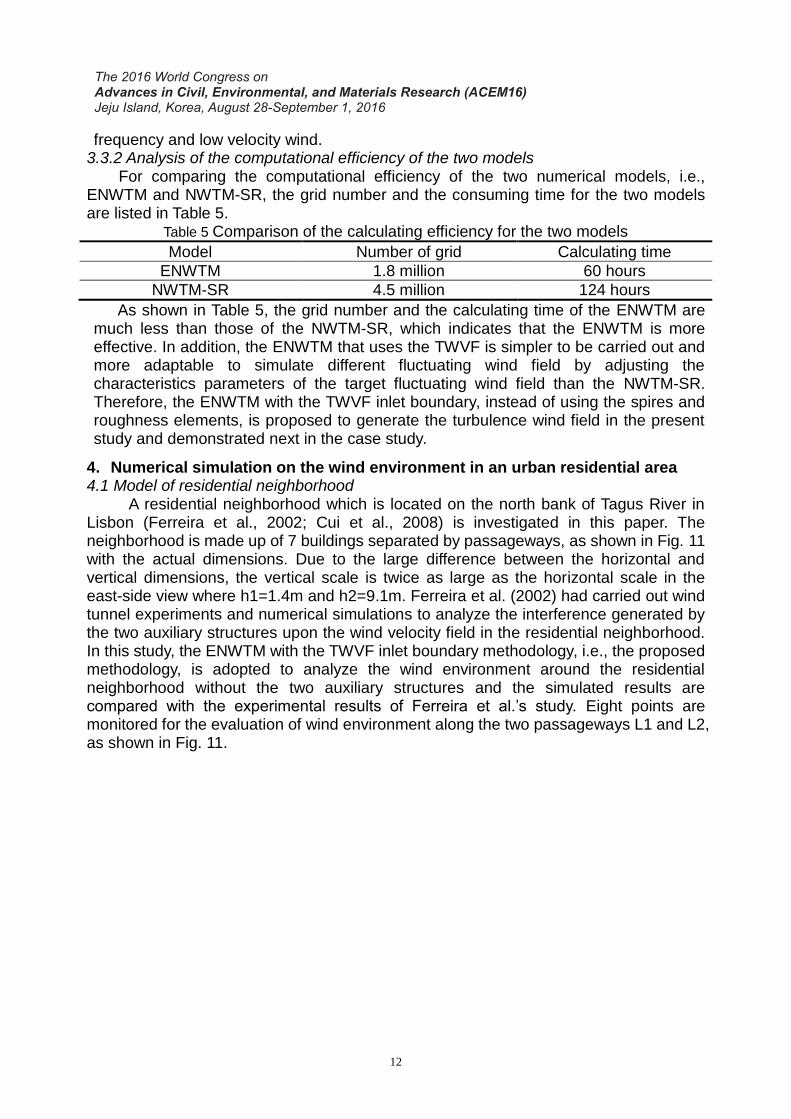
frequency and low velocity wind. 3.3.2 Analysis of the computational efficiency of the two models

For comparing the computational efficiency of the two numerical models, i.e., ENWTM and NWTM-SR, the grid number and the consuming time for the two models are listed in Table 5.

Table 5 Comparison of the calculating efficiency for the two models

Model Number of grid Calculating time

ENWTM 1.8 million 60 hours

NWTM-SR 4.5 million 124 hours

As shown in Table 5, the grid number and the calculating time of the ENWTM are much less than those of the NWTM-SR, which indicates that the ENWTM is more effective. In addition, the ENWTM that uses the TWVF is simpler to be carried out and more adaptable to simulate different fluctuating wind field by adjusting the characteristics parameters of the target fluctuating wind field than the NWTM-SR. Therefore, the ENWTM with the TWVF inlet boundary, instead of using the spires and roughness elements, is proposed to generate the turbulence wind field in the present study and demonstrated next in the case study.

4. Numerical simulation on the wind environment in an urban residential area 4.1 Model of residential neighborhood A residential neighborhood which is located on the north bank of Tagus River in Lisbon (Ferreira et al., 2002; Cui et al., 2008) is investigated in this paper. The neighborhood is made up of 7 buildings separated by passageways, as shown in Fig. 11 with the actual dimensions. Due to the large difference between the horizontal and vertical dimensions, the vertical scale is twice as large as the horizontal scale in the east-side view where h1=1.4m and h2=9.1m. Ferreira et al. (2002) had carried out wind tunnel experiments and numerical simulations to analyze the interference generated by the two auxiliary structures upon the wind velocity field in the residential neighborhood. In this study, the ENWTM with the TWVF inlet boundary methodology, i.e., the proposed methodology, is adopted to analyze the wind environment around the residential neighborhood without the two auxiliary structures and the simulated results are compared with the experimental results of Ferreira et al.’s study. Eight points are monitored for the evaluation of wind environment along the two passageways L1 and L2, as shown in Fig. 11.

13

(a) Top-side view

(b) East-side view

Fig. 11 Sketch map of the residential neighborhood under study

4.2 Grid mesh and boundary conditions To adjust the wind direction easily, a circle calculation domain is adopted in this

study, as shown in Fig. 12 (a). The calculation domain is divided into 8 parts equally from the external border. Therefore, only small changes are needed to adjust the wind direction. The domain is meshed into hexahedral grids with O-block method, as shown in Fig. 12 (b), the diameter of the calculation domain is 900m, and the total number of grids is about 4.6 million.

(a) Computational domain

(b) Computational mesh

Fig. 12 Computational domain and mesh

The inflow boundary conditions of the numerical simulation are the same as those of the wind tunnel experiments carried out by Ferreira et al. (2002). The average wind

velocity of the flow is calculated with the formula 𝑢/𝑈0 = (𝑧

ℎ0)𝛼

, where ℎ0=70 m is the

reference height; 𝑈0=11 m/s is the mean wind velocity at the height of h0;and the

exponent 𝛼 is 0.11. The inlet turbulence intensity obtained from the wind tunnel experiments (Ferreira et al., 2002), is shown in Fig. 13.

P1 P2 P3 P4 P5 P6

AP8

P1 P2 P3 P4 P5 P6

CP8

L1

L2

h1

h2

x

217.5m

200.4

m

y

N S

E

W

z

1 4

2 5

63

7

3 6 7

B D

P7

P7

4

2 5

63

7

3 6 7

P1 P2 P3 P4 P5 P6 P7 P8

P1 P2 P3 P4 P5 P6 P7 P8

L1

L2

h1

h2

x

217.5m

200.4

m

y

N S

E

W

z

1

14

0.0

0.2

0.4

0.6

0.8

1.0

1.2

0.0 5 10 15 20

z/h0

Iu(%) Fig. 13 Measured turbulence intensity on the inlet boundary

As discussed earlier, in the proposed methodology, the fluctuating flow information is generated by the WAWS method according to the turbulence intensity and added on the inlet boundary in LES using the ENWTM. To reflect the superiority of the proposed methodology, for a comparison, the common method in which the velocity without considering the wind fluctuations in the form of velocity profile is inputted on the inlet boundary is also adopted here to analyze the wind environment around the residential neighborhood. The numerical simulation on the wind environment around the residential neighborhood is carried out with four cases with different boundary conditions, as shown in Table 6.

Table 6 Simulation cases

Cases Wind Direction The inputting method of the wind field

1 North The proposed methodology

2 North The common method without inlet fluctuations

3 Northeast The proposed methodology

4 Northwest The proposed methodology

4.3 Calculating results For Case 1, the mean wind velocity profiles of points P1-P8 along the passageways

L1 and L2 are obtained and compared with the wind tunnel experimental results measured by Ferreira et al. (2002), as shown in Fig. 14, where V is the wind velocity magnitude, V0 is the inlet flow conditions at the same level and the velocity difference is normalized by the wind velocity U0. The mean wind velocity profiles at different positions in the residential neighborhood are well reflected in these figures.

From Fig. 14, it can be observed that the simulation results in this study agree well with the experimental results measured by Ferreira et al. (2002) for passageways L1 and L2. The buildings in the residential neighborhood have obvious influence on the mean wind velocity profiles, especially for the near ground. The mean wind velocity declines obviously near the ground. The higher the height is, the smaller the decline tendency of the mean wind velocity is. As the height is twice or more the height of the buildings, the difference between the mean wind velocity of the monitoring point and the inlet flow conditions at the same level is small. The mean wind velocity along the horizontal direction declines too due to the influence of the friction of buildings. Meanwhile, the longer the horizontal distance from the inlet is, the larger the influence on the average wind velocity is.

15

（a）Velocity profiles along the passageways L1 (b) Velocity profiles along the passageways L2

(“□” stands for the measured value of 7-hole probe in the wind tunnel experiment；“ ” is the measured value of

hot-wire anemometer“ ”is the simulated wind velocity) Fig. 14 Velocity profiles at the monitoring points along the passageways

Fig. 15 presents the turbulence intensity profiles at the monitoring points along the passageways L1 and L2 for Case 1. From Fig. 15, it can be observed that the turbulence intensities increase obviously near the ground. When the height is twice or more the height of the buildings, the turbulence intensity of the monitoring points is the same as that of the inlet level. Meanwhile, it can be found that the turbulence intensities are also influenced by the horizontal distance from the inlet and the turbulence intensity near the ground increases with the increase of the distance.

(a) Turbulence intensity profiles along the passageway L1

(b) Turbulence intensity profiles along the passageway L2

Fig. 15 Turbulence intensity profiles at the monitoring points along the passageways

16

In order to understand the influence of the inlet fluctuations, the root mean square (RMS) values of the velocities simulated at points A ~ D for Case 1 and Case 2 are compared and shown in Fig. 16. It clearly found that the RMS values of velocities for Case 1 (with the inlet fluctuation) are larger than those for Case 2 (without the inlet fluctuation) on the whole. The RMS values of velocities increase at first, then decrease and trend to be a constant value with the dimensionless height z/h0.It can be seen from Fig. 16(a) that the value trends to be about 1.5 m/s when z/h0 is larger than 0.6 for Case 1, but is close to zero when z/h0 is larger than 0.4 for Case 2. Similar change law can be found in Figs. 16 (b) ~ 16(d). From the above analysis, it indicates that the turbulence in the flow field for Case 1 is developed better than that for Case 2. Therefore, the inclusion of the inlet fluctuations is very important for generating a reasonable turbulent wind field, which in turn plays a significant role in the process of contaminant dispersion among groups of buildings.

0.0

0.2

0.4

0.6

0.8

1.0

1.2

1.4

1.6

1.8

-0.5 0.0 0.5 1.0 1.5 2.0 2.5 3.0 3.5

Urms

z/h

0

without inlet fluctuations

with inlet fluctuations

0.0

0.2

0.4

0.6

0.8

1.0

1.2

1.4

1.6

1.8

0.0 0.5 1.0 1.5 2.0 2.5 3.0

Urms

z/h

0

without inlet fluctuations

with inlet fluctuations

(a) Point A (b) Point B

0.0

0.2

0.4

0.6

0.8

1.0

1.2

1.4

1.6

1.8

0.0 0.5 1.0 1.5 2.0 2.5 3.0

Urms

z/h

0

without inlet fluctuations

with inlet fluctuations

0.0

0.2

0.4

0.6

0.8

1.0

1.2

1.4

1.6

-0.5 0.0 0.5 1.0 1.5 2.0 2.5 3.0 3.5

Urms

z/h

0

without inlet fluctuations

with inlet fluctuations

(c) Point C (d) Point D

Fig. 16 Velocity root mean square

The average wind velocity in the residential neighborhood must be kept in a certain range, i.e., cannot be too high or too low. A too high wind velocity will make pedestrians uncomfortable while a too low wind velocity will impede ventilation resulting in the accumulation of pollutants and thus influence people’s health. It is pointed out in the concerned code (JGJT229-2010) that when the average wind velocity reaches to 5m/s, people will feel uncomfortable. In order to analyze the wind environment at the pedestrian level in detail, the velocity contour and velocity streamlines of the wind field

17

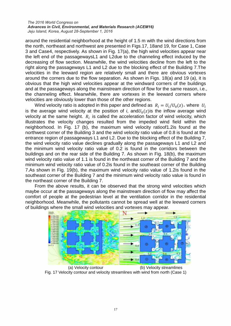
around the residential neighborhood at the height of 1.5 m with the wind directions from the north, northeast and northwest are presented in Figs.17, 18and 19, for Case 1, Case 3 and Case4, respectively. As shown in Fig. 17(a), the high wind velocities appear near the left end of the passagewaysL1 and L2due to the channeling effect induced by the decreasing of flow section. Meanwhile, the wind velocities decline from the left to the right along the passageways L1 and L2 due to the blocking effect of the Building 7.The velocities in the leeward region are relatively small and there are obvious vortexes around the corners due to the flow separation. As shown in Figs. 18(a) and 19 (a), it is obvious that the high wind velocities appear at the windward corners of the buildings and at the passageways along the mainstream direction of flow for the same reason, i.e., the channeling effect. Meanwhile, there are vortexes in the leeward corners where velocities are obviously lower than those of the other regions.

Wind velocity ratio is adopted in this paper and defined as 𝑅𝑖 = 𝑈𝑖/𝑈0(𝑧)，where 𝑈𝑖 is the average wind velocity at the position of i, and𝑈0(𝑧)is the inflow average wind

velocity at the same height. 𝑅𝑖 is called the acceleration factor of wind velocity, which illustrates the velocity changes resulted from the impeded wind field within the neighborhood. In Fig. 17 (b), the maximum wind velocity ratioof1.2is found at the northwest corner of the Building 3 and the wind velocity ratio value of 0.8 is found at the entrance region of passageways L1 and L2. Due to the blocking effect of the Building 7, the wind velocity ratio value declines gradually along the passageways L1 and L2 and the minimum wind velocity ratio value of 0.2 is found in the corridors between the buildings and on the rear side of the Building 7. As shown in Fig. 18(b), the maximum wind velocity ratio value of 1.1 is found in the northeast corner of the Building 7 and the minimum wind velocity ratio value of 0.2is found in the southeast corner of the Building 7.As shown in Fig. 19(b), the maximum wind velocity ratio value of 1.2is found in the southeast corner of the Building 7 and the minimum wind velocity ratio value is found in the northeast corner of the Building 7.

From the above results, it can be observed that the strong wind velocities which maybe occur at the passageways along the mainstream direction of flow may affect the comfort of people at the pedestrian level at the ventilation corridor in the residential neighborhood. Meanwhile, the pollutants cannot be spread well at the leeward corners of buildings where the small wind velocities and vortexes may appear.

(a) Velocity contour (b) Velocity streamlines Fig. 17 Velocity contour and velocity streamlines with wind from north (Case 1)

18

(a) Velocity contour (b) Velocity streamlines Fig. 18 Velocity contour and velocity streamlines with wind from northeast (Case 3)

(a) Velocity contour (b) Velocity streamlines Fig. 19 Velocity contour and velocity streamlines with wind from northwest (Case 4)

0.0

0.2

0.4

0.6

0.8

1.0

1.2

1.4

1.6

0 2 4 6 8 10 12 14

k

z/h

0

Point A

Point B

Point C

Point D

Fig. 20 Profile of turbulent kinetic energy (Case 1)

The turbulence intensity is the other factor which can affect the comfort of people at the pedestrian level in the residential neighborhood. The distribution of the turbulent kinetic energy (TKE) along the height can reflect the spatial variation of the turbulence intensity. For facilitating the understanding of the distribution of the TKE around the residential neighborhood, the profiles of the TKE at the points A-D (defined in Fig. 11) for Case 1 are investigated and shown in Fig. 20.As shown in Fig. 20, the TKE increases at

19

first, then decreases with the dimensionless height z/h0 and trends to be a constant value (i.e., the TKE of the free flow). For points A and Cat the passageways L1 and L2, the maximum values of TKEs occur at the height of 1.5 m (i.e., z/h0 is 0.021), which is about the pedestrian level height, and the values gradually decrease with the height and trend to be close to the TKE of the free flow at about the height of 18 m. For points B and D at the passageways which are perpendicular to the direction of the incoming flow, the maximum values of TKEs occurred at about the height of 20 m (i.e., z/h0 is about 0.3) on the building top in the strong shear region, and the values gradually decrease with the height and trend to be close to the TKE of the free flow at about the height of 56 m. From the above analysis, it indicates that the comfort degree of people at the pedestrian level at the passageways L1 and L2 is lower than that at other positions not only because of the higher average wind velocity, but also the higher TKE at the pedestrian level at these passageways.

5. Conclusions An inflow turbulence generating method is presented in the present study based on

the weighted amplitude wave superposition (WAWS) method, which can generate a fluctuating wind flow field satisfying any desired target spectrum by the technique of WAWS. Then, the proposed approach is successfully applied to simulate the wind environment around a real residential neighborhood and the numerical results are compared with the wind tunnel experimental results. Based on the analysis results, following conclusions can be drawn:

(1) The inflow turbulent flow field with the prescribed spectra can be well generated using the proposed methodology. By the comparison of the numerical results with the wind tunnel experimental results, it is revealed that the inflow turbulence generating method based on the weighted amplitude wave superposition (WAWS) method is accurate and can satisfy the requirement of the engineering application. And then, by comparing the calculating efficiency of the proposed methodology with that of the NWTM-SR approach, it is found that the proposed methodology is more efficient and adaptable.

(2)The mean wind velocity and turbulence intensity profiles at different positions in the residential neighborhood are investigated and validated by comparing with the experimental results. The results show that the mean wind velocity declines while turbulence intensity increases obviously on the near ground. When the height is twice or more the height of the buildings, the mean wind velocity and turbulence intensity of the monitoring point is essentially the same as that of the inlet flow at the same level. The average wind velocity and turbulence intensity are also influenced by the horizontal distance from the inlet.

(3)By comparing the root mean square (RMS) values of the velocities at the points in the residential neighborhood, it is observed that inclusion of the inlet fluctuations is very important for generating a reasonable turbulent wind field, which in turn plays a significant role in the process of contaminant dispersion among groups of buildings.

(4) By the analysis of the average wind velocity at the height of 1.5 m and the TKE around the residential neighborhood, it is observed that the stronger wind velocities and the higher TKEs occur at the passageways along the mainstream direction of flow which may affect the comfort of people at the pedestrian level in the residential neighborhood. The small wind velocities and vortexes appear at the leeward corners of buildings which

20

may affect the spreading of the pollutants.

Acknowledgements

The work described in this paper is supported by the key basic research project (973 project) of P. R. China, under contract No. 2015CB057706 and 2015CB057701. The authors would also like to gratefully acknowledge the supports from the National Science Foundation of China (Project 51278069; 51208067; 51178066). The work described in this paper is also supported by the Open Foundation for the Key Laboratory of Ministry of Education of Province and Ministry Co-construction on security control of bridge engineering of Changsha University of Science and Technology (12KB01). Reference Britter R. E. and Hanna S. R. (2003), “Flow and dispersion in urban area”, J. Annu Rev Fluid Mech, 35: 469-495. Castro H.G. and Paz R. R. (2012), “A time and space correlated turbulence synthesis method for large eddy simulations”, J. Comput Phys. 235:742–763. Chung Y. M. and Sung H. J. (1997), “Comparative study of inflow conditions for spatially evolving simulation”, AIAA Joural, 35(2):269-274. CuiG. X., Zhang Z. X. and Xu C. X. (2013), “Research advances in large eddy simulation of urban atmospheric environment”, J. Adv. Mech. 43(3):295-328. (in Chinese) Cui, G. X., Shi, R. F., Wang, Z.S, Xu, C. X. and Zhang, Z. X. (2008), “Large Eddy Simulation of Urban Micro-atmospheric Environment”, J. Science in china.38(6):626-636. (in Chinese) G. Deodatis. (1996), “Simulation of ergodic multivariate stochastic processes Engineering Mechanics”, ASCE, 122(8): 778-787. Ferreira A. D., Sousa A. C. M. and Viegas D. X. (2002), “Prediction of building interference effects on pedestrian level comfort”, J. Wind Eng. Ind. Aerodyn, 90: 305-319. Fluent Inc. (2009), “Fluent user’s guide”, version: ansys12.0. USA. Fureby C. (1996), “On subgrid scale modeling in large eddy simulations of compressible fluid flow”, J. Phys. Fluids, 8: 1301–1311. Germano M., PiomelliU., MoinP. and Cabot W. H., (1991), “A dynamics subgrid-scale eddy viscosity model”, J. Phys. FluidsA, 3(7): 1760-1765. Gousseau P., Blocken B. and van Heijst G. J. F. (2012), “CFD simulation of pollutant dispersion around isolated buildings: On the role of convective and turbulent mass fluxes in the prediction accuracy”, Journal of Hazardous Materials, 194: 422-434. Guo Y. J., RyuichiroYoshie, Taichi Shirasawa and Jin X. Y. (2012), “Inflow turbulence generation for large eddy simulation in non-isothermal boundary layers”, J. Wind Eng. Ind. Aerodyn, 104(106): 369-378. Han Yan.(2007), “Study on Complex Aerodynamic Admittance Functions and Refined Analysis of Buffeting Response of Bridge”, Hunan university doctoral dissertation. (in Chinese) Hanna S. R., Tehranian S., Carissimo B., MacDonald R. W. and Lohner R.(2002), “Comparisons of model simulations with observations of mean flow and turbulence within simple obstacle arrays”, J. Atmospheric Environment., 36: 5067-5079. H. Noda and A. Nakayama. (2003), “Reproducibility of flow past two-dimensional rectangular cylinders in a homogeneous turbulent flow by LES”, J. Wind Eng. Ind. Aerodyn. 91: 265–278 Hemon P. and Santi F. (2007), “Simulation of a spatially correlated turbulent velocity field using biorthogonal decomposition”, J. Wind Eng. Ind.Aerodyn.95 (1): 21-29. Hoshiya M. (1972), “Simulation of multi-correlated random processes and application to structural vibration problems”, Proceedings of JSCE, 204: 121-128. Huang S.H., Li Q.S. and Wu J. R. (2010), “A general inflow turbulence generator for large eddy simulation”, J .Wind Eng. Ind. Aerodyn ,98: 600-617. Jiang W. M. and Miao S. G. (2004), “30 years review and perspective of the research on the large eddy simulation and atmospheric boundary layer”, J. Advances in Natural Sciences,14:11-19. (in

21

Chinese) Kataoka H. and Mizuno M. (2002), “Numerical flow computation around aeroelastic 3D square cylinder using inflow turbulence”, Wind and Structures 5: 379-392. Keating A., Piomelli U., Balaras E.and Kaltenbach H. J., (2004), “A priori and a posteriori tests of inflow conditions for large-eddy simulation”, J. Phys. Fluids,16:46-96. Kondo K., Murakami S., Mochida A., (1997), “Generation of velocity fluctuations for inflow boundary condition of LES”, J. Wind Eng. Ind. Aerodyn., 67&68:51-64. Kondo H., Asahi K., Tomizuka T. and Suzuki M. (2006), “Numerical analysis of diffusion around a suspended expressway by a multi-scale CFD model”, J. Atmospheric Environment, 40; 2852-2859. Kraichnan R. H. (1970), “Diffusion by a random velocity field”, J. Phys Fluids;13(1):22–31. Lund T. S., Wu X. H. and Squires K. D. (1998), “Generation of turbulent inflow data for spatially-developing boundary layer simulations”, J. Comput. Phys.,140: 233–258. Maruyama T. and Morikawa H. (1994), “Numerical simulation of wind fluctuation conditioned by experimental data in turbulent boundary layer”, C. Proceedings of the 13th Symposium on Wind Engineering, 573–578. Mathey F., Cokljat D., Bertoglio J. P. and Sergent E. (2006), “Assessment of the vortex method for large eddy simulation inlet conditions”, Progress in Computational Fluid Dynamics,6:59-67. Ministry of Housing and Urban-Rural Development (MOHUR), “Code for green design of civil buildings”, JGJT229-2010, China. Nozawa K. and Tamura T. (2002), “Large eddy simulation of the flow around a low-rise building immersed in a rough-wall turbulent boundary layer”, J. Wind Eng. Ind. Aerodyn., 90:1151-1162. Pang J. B. and Lin Z. X. and Chen Y. (2004), “Discussion on the simulation of atmospheric boundary layer with spires and roughness elements in wind tunnels”, Experiments and Measurements in Fluid Mechanics, 18(2): 32-37. (in Chinese) Smirnov R., Shi S. and Celik I. (2001), “Random flow generation technique for large eddy simulations and particle-dynamics modeling”, J. Fluids Eng.,123:359-371. Tabor G.R and Baha-Ahmadi M.H,(2010), “Inlet conditions for large eddy simulation: a review”, Computer & Fluids,39(4): 553-567. Tamura T. (2000), “Towards practical use of LES in wind engineering”, J. Wind Eng. Ind. Aerodyn, 96(10-11):1451-1471. Tamura T., Tsubokura M., Cao S. and Furusawa T. (2003), “LES of spatially-developing stable/unstable stratified turbulent boundary layers”, Direct and Large-Eddy Simulation,5: 65-66. Tominaga Y., Mochida A., Murakami S., and Sawaki S. (2008), “Comparison of various revised k- models and LES applied to flow around a high-rise building model with 1:1:2 shape placed within the surface boundary layer”, J. Wind Eng. Ind. Aerodyn.,96:389-411. Xie Z. T. and Castro I. P. (2008), “Efficient generation of inflow conditions for large eddy simulation of street-scale flows”, Flow Turbulence and Combustion, 81: 449-470. Yan B.W., Li Q. S.(2015), “Inflow turbulence generation methods with large eddy simulation for wind effects on tall buildings”, J. Computers & Fluids,116: 158-175. Yu R.X. and Bai X.S. (2014), “A fully divergence-free method for generation of inhomogeneous and anisotropic turbulence with large spatial variation”, J. Comput Phys, 256:234-253.