Language Reference Guide - University of California, Davisanimalscience2.ucdavis.edu/nut254/Language...
177
acslXtreme ™ Language Reference Guide Version 1.3 February 2003 The AEgis Technologies Group, Inc. 631 Discovery Drive Huntsville, AL 35806 U.S.A.
Transcript of Language Reference Guide - University of California, Davisanimalscience2.ucdavis.edu/nut254/Language...

acslXtreme™
Language ReferenceGuide
Version 1.3February 2003
The AEgis Technologies Group, Inc.631 Discovery DriveHuntsville, AL 35806
U.S.A.

acslXtreme™ Language Reference GuideCopyright (c) 2003 The AEgis Technologies Group, Inc.All Rights Reserved.Printed in the United States of America.
ACSL is a registered trademark of The AEgis Technologies Group, Inc.AcslXtreme is a trademark of The AEgis Technologies Group, Inc.PowerBlock is a trademark of The AEgis Technologies Group, Inc.
Microsoft, Windows, Microsoft .NET, and Microsoft Internet Explorer are either registered trademarks or trademarks of Microsoft Corporation in the United States and/or other countries.
FLEXlm is a registered trademark of Globetrotter Software, Inc., A Macrovision Company
All other brand and product names mentioned herein are the trademarks and registered trademarks of their respective owners.
Information in this document is subject to change without notice. The software described in this document is furnished under a license agreement. The software and this documentation may be used only in accor-dance with the terms of those agreements.
The AEgis Technologies Group, Inc.631 Discovery Drive Huntsville, AL 35806U. S. A.
fax: 512-615-3574email: [email protected]: http://www.acslXtreme.com
February 2003

Chapter 1 Introduction1.1 Simulation Language ............................................................................. 1-11.2 The Code Window ................................................................................. 1-11.3 Job processing ...................................................................................... 1-21.4 Conventions ........................................................................................... 1-21.5 Language features ................................................................................. 1-21.6 Coding procedure .................................................................................. 1-61.7 Reserved names ................................................................................... 1-6
Chapter 2 Language Elements2.1 Introduction ............................................................................................ 2-12.2 Constants .............................................................................................. 2-12.3 Variables ................................................................................................ 2-32.4 Labels .................................................................................................... 2-42.5 Expressions ........................................................................................... 2-5
Chapter 3 Program Structure3.1 Implicit and explicit structure ................................................................. 3-13.2 Program flow ......................................................................................... 3-23.3 Program sorting ..................................................................................... 3-43.4 Proram Structure Preset of User Variables ........................................... 3-53.5 Preset of user variables ......................................................................... 3-63.6 Preset of derivatives .............................................................................. 3-6
Chapter 4 acslXtreme Statements4.1 Introduction ............................................................................................ 4-14.2 ABS ....................................................................................................... 4-54.3 ACOS .................................................................................................... 4-54.4 AINT ...................................................................................................... 4-64.5 ALGORITHM ......................................................................................... 4-64.6 ANINT .................................................................................................. 4-144.7 ASIN .................................................................................................... 4-154.8 Assignment statements ....................................................................... 4-154.9 ATAN ................................................................................................... 4-164.10 ATAN2 ................................................................................................. 4-174.11 BCKLSH .............................................................................................. 4-174.12 BOUND ................................................................................................ 4-184.13 CALL .................................................................................................... 4-184.14 CHARACTER ...................................................................................... 4-194.15 CINTERVAL ........................................................................................ 4-194.16 CMPXPL .............................................................................................. 4-224.17 Comment (!) ......................................................................................... 4-234.18 CONSTANT ......................................................................................... 4-234.19 Continuation (&) ................................................................................... 4-254.20 CONTINUE .......................................................................................... 4-264.21 COS ..................................................................................................... 4-264.22 DBLE ................................................................................................... 4-27
acslXtreme Language Reference Manual 1
4.23 DBLINT ................................................................................................ 4-274.24 DEAD ................................................................................................... 4-294.25 DELAY ................................................................................................. 4-294.26 DELSC ................................................................................................. 4-314.27 DELVC ................................................................................................. 4-324.28 DERIVATIVE ....................................................................................... 4-334.29 DERIVT ............................................................................................... 4-344.30 DIM ...................................................................................................... 4-354.31 DIMENSION ........................................................................................ 4-364.32 DISCRETE .......................................................................................... 4-374.33 DO ....................................................................................................... 4-384.34 DOUBLE PRECISION ......................................................................... 4-394.35 DYNAMIC ............................................................................................ 4-394.36 END ..................................................................................................... 4-404.37 ERRTAG .............................................................................................. 4-404.38 EXP ..................................................................................................... 4-414.39 FCNSW ............................................................................................... 4-414.40 GAUSI, UNIFI ...................................................................................... 4-424.41 GAUSS ................................................................................................ 4-434.42 GO TO ................................................................................................. 4-434.43 HARM .................................................................................................. 4-444.44 HISTORY ............................................................................................. 4-454.45 IF, IF-THEN-ELSE ............................................................................... 4-464.46 IMPLC .................................................................................................. 4-484.47 IMPVC ................................................................................................. 4-514.48 INCLUDE ............................................................................................. 4-524.49 INITIAL ................................................................................................ 4-534.50 INT ....................................................................................................... 4-544.51 INTEG .................................................................................................. 4-554.52 INTEGER ............................................................................................. 4-574.53 INTERVAL ........................................................................................... 4-574.54 INTVC .................................................................................................. 4-584.55 LEDLAG .............................................................................................. 4-594.56 LIMINT ................................................................................................. 4-604.57 LOG ..................................................................................................... 4-624.58 LOG10 ................................................................................................. 4-624.59 LOGICAL ............................................................................................. 4-634.60 LSW, RSW .......................................................................................... 4-634.61 MACRO ............................................................................................... 4-644.62 MAX ..................................................................................................... 4-644.63 MAXTERVAL, MINTERVAL ................................................................ 4-644.64 MERROR, XERROR ........................................................................... 4-664.65 MIN ...................................................................................................... 4-674.66 MINTERVAL ........................................................................................ 4-684.67 MOD .................................................................................................... 4-684.68 NINT .................................................................................................... 4-684.69 NSTEPS .............................................................................................. 4-694.70 OU ...................................................................................................... 4-704.71 PARAMETER ...................................................................................... 4-72
2 acslXtreme Language Reference Manual
4.72 PROCEDURAL .................................................................................... 4-734.73 PROGRAM .......................................................................................... 4-754.74 PTR ..................................................................................................... 4-754.75 PULSE ................................................................................................. 4-764.76 QNTZR ................................................................................................ 4-774.77 RAMP .................................................................................................. 4-774.78 REAL ................................................................................................... 4-784.79 REALPL ............................................................................................... 4-784.80 RESET ................................................................................................. 4-794.81 RSW .................................................................................................... 4-804.82 RTP ..................................................................................................... 4-804.83 SAVE ................................................................................................... 4-814.84 SCALE ................................................................................................. 4-814.85 SCHEDULE ......................................................................................... 4-824.86 SCHEDULE Time Event Specification ................................................ 4-864.87 SCHEDULE State Event Specification ................................................ 4-884.88 SCHEDULE State Event Mechanization ............................................. 4-884.89 Separator (;) ........................................................................................ 4-924.90 SIGN .................................................................................................... 4-924.91 SIN ....................................................................................................... 4-934.92 SORT ................................................................................................... 4-934.93 SQRT ................................................................................................... 4-934.94 STEP ................................................................................................... 4-954.95 TABLE ................................................................................................. 4-964.96 TAN ................................................................................................... 4-1004.97 TERMINAL ........................................................................................ 4-1004.98 TERMT .............................................................................................. 4-1014.99 TRAN ................................................................................................ 4-1024.100 TRANZ ............................................................................................... 4-1044.101 Type ................................................................................................... 4-1064.102 UNIF .................................................................................................. 4-1084.103 UNIFI ................................................................................................. 4-1084.104 VARIABLE ........................................................................................ 4-1084.105 XERROR ........................................................................................... 4-108
Chapter 5 Macro Language5.1 Introduction ............................................................................................ 5-15.2 Macro definitions ................................................................................... 5-35.3 Macro definition header ......................................................................... 5-35.4 Macro directive statements .................................................................... 5-55.5 Macro examples .................................................................................. 5-115.6 Macro invocation ................................................................................. 5-17
Appendix A Programming Style
Appendix B General Purpose Utilities
Appendix C acslXtreme System Symbols
acslXtreme Language Reference Manual 3

4 acslXtreme Language Reference Manual
Introduction Simulation Language
Chapter 1 Introduction
1.1 Simulation LanguageSimulation of physical systems is a standard analysis tool used to evaluate designs prior to actual construction. acslXtreme provides a simple method of modeling systems described by time-dependent, nonlinear differential equations and/or transfer functions.1 Typical continuous simulation applications include control system design, chemical process representation, missile and aircraft simulation, power plant dynamics, biomedical systems, vehicle handling, microprocessor controllers, fluid flow, and heat transfer analysis. Users can derive code for the simulation model from block diagrams, mathematical equations, conventional Fortran statements, etc.
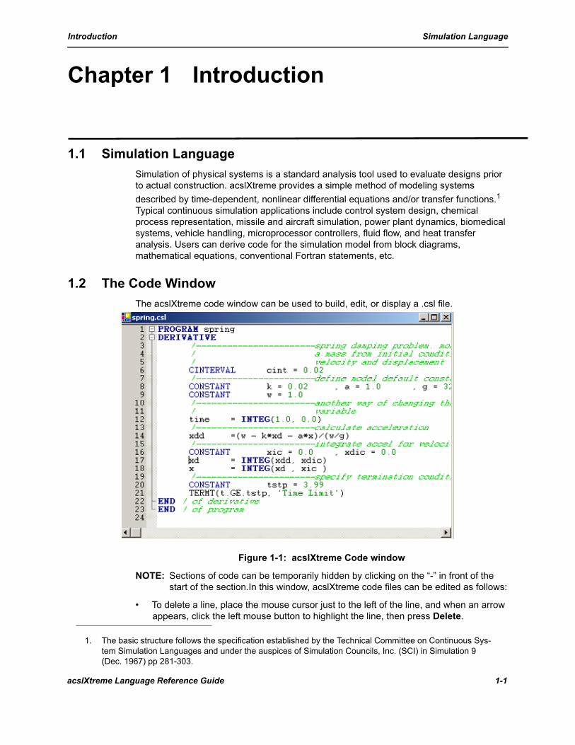
1.2 The Code WindowThe acslXtreme code window can be used to build, edit, or display a .csl file.
Figure 1-1: acslXtreme Code window
NOTE: Sections of code can be temporarily hidden by clicking on the “-” in front of the start of the section.In this window, acslXtreme code files can be edited as follows:
• To delete a line, place the mouse cursor just to the left of the line, and when an arrow appears, click the left mouse button to highlight the line, then press Delete.
1. The basic structure follows the specification established by the Technical Committee on Continuous Sys-tem Simulation Languages and under the auspices of Simulation Councils, Inc. (SCI) in Simulation 9 (Dec. 1967) pp 281-303.
acslXtreme Language Reference Guide 1-1
Introduction Job processing
• To add a line, place the cursor at the end of the previous line, then press Enter.• To add text, place the cursor at the location where the text should be and start typing.• To copy/paste text, • Select the text to be copied.
- Press Ctrl-C or right-click and select Copy from the pop-up menu. - Place the cursor where the text needs to be pasted.- Press Ctrl-V or right-click and select Paste from the pop-up menu.
• To drag-and drop text, select the text, then click and hold the left mouse button while dragging the text to the new position.
1.3 Job processingInputs to acslXtreme are in two parts.
Program—defines the system being modeled. The program is read by the acslXtreme translator, which translates it to a C or Fortran source code file. The source code is then compiled and linked with the acslXtreme runtime library.
Simulation Control Commands—simulation control commands, which exercise the model, can be submitted in batch mode or entered interactively. Interactively you can run the simulation, look at the results, and change constants to experiment with the model; for example, trying different spring constants or actuator limits.
At this point, the compiled simulation can be run using one of the following methods:
• interactively at the cntrl> command prompt• by executing a command file or batch process• by selecting a toolbar or menu item which results in execution of the simulation
1.4 ConventionsThis guide uses different typefaces to help distinguish between different conventions as follows:
1.5 Language featuresThe acslXtreme language uses free-form input function generation of up to three variables, and independent error control on each integrator. Working from an equation description of the problem, acslXtreme statements are written to describe the proposed system. Plotting flexibility is provided by using a number of external forcing functions. Many simulation-oriented operators such as variable time delay, dead zone, backlash, and quantization are included. Global single or double-precision calculation can be selected.
Courier Command lines
Bold Menu items, keyboard keys
Italics Variables
1-2 acslXtreme Language Reference Guide
Introduction Language features
The sorting of the continuous model equations is a feature of acslXtreme, in contrast to general purpose programming languages such as Fortran where program execution depends on statement order.
The language consists of a set of arithmetic operators, standard functions, a set of special acslXtreme statements, and a MACRO capability. The MACRO capability allows extension of the special acslXtreme statements, either at the system level for each installation, or for each individual user.
1.5.1 Operators and functionsThe arithmetic, relational, and logical operators are described in Chapter 2. The functions, listed in Chapter 4, consist of special acslXtreme operators such as QNTZR (quantization), UNIF (uniform random number), etc. In addition, library functions are available; e.g., SQRT (square root), MOD (modulus), etc.
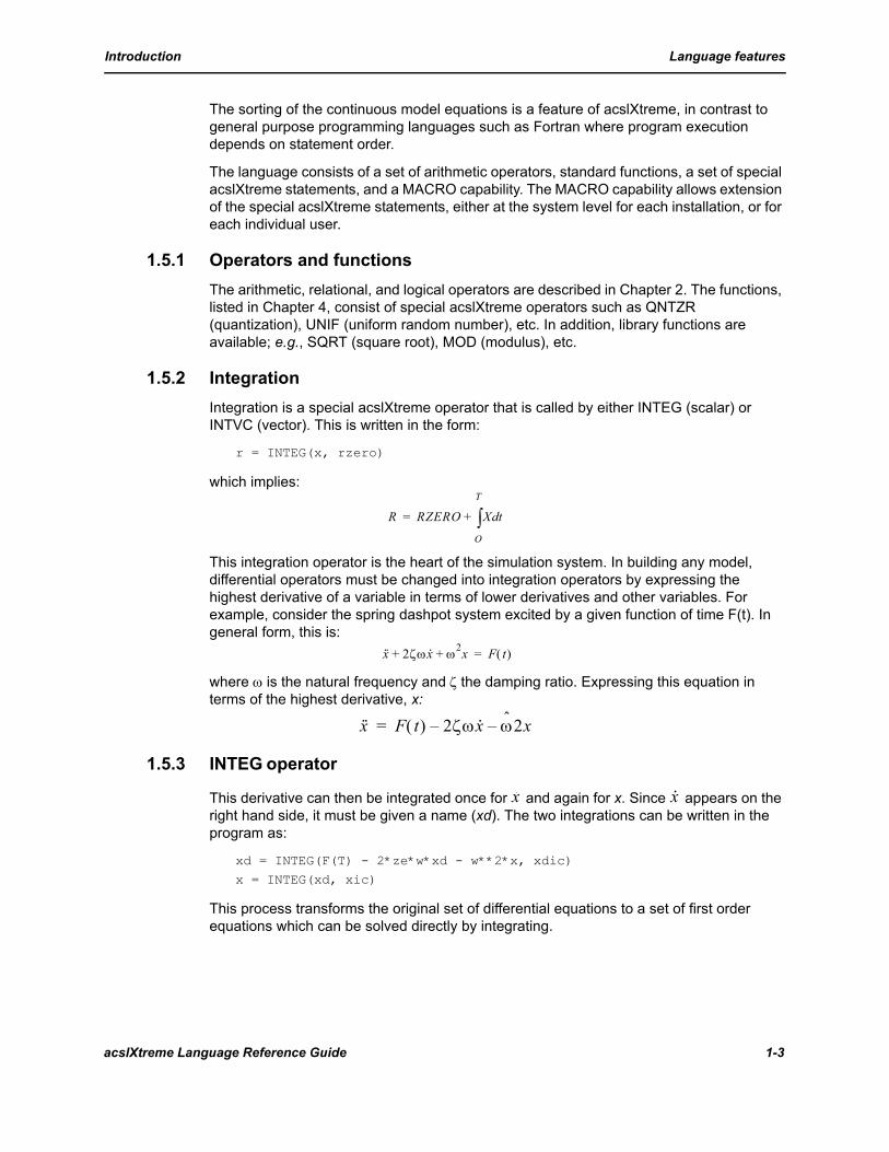
1.5.2 IntegrationIntegration is a special acslXtreme operator that is called by either INTEG (scalar) or INTVC (vector). This is written in the form:
r = INTEG(x, rzero)
which implies:
This integration operator is the heart of the simulation system. In building any model, differential operators must be changed into integration operators by expressing the highest derivative of a variable in terms of lower derivatives and other variables. For example, consider the spring dashpot system excited by a given function of time F(t). In general form, this is:
where ω is the natural frequency and ζ the damping ratio. Expressing this equation in terms of the highest derivative, x:
1.5.3 INTEG operator
This derivative can then be integrated once for and again for x. Since appears on the right hand side, it must be given a name (xd). The two integrations can be written in the program as:
xd = INTEG(F(T) - 2*ze*w*xd - w**2*x, xdic)
x = INTEG(xd, xic)
This process transforms the original set of differential equations to a set of first order equations which can be solved directly by integrating.
R RZERO X tdO
T
∫+=
x·· 2ζωx· ω2x+ + F t( )=
x·· F t( ) 2ζωx·– ω̂2x–=
x· x·
acslXtreme Language Reference Guide 1-3

Introduction Language features
1.5.4 Redundant state variablesBe careful to avoid introducing redundant state variables in the transformation process. In
the above sequence, the reference to x.(xd) could have been avoided by calculating (xdd) directly and embedding an INTEG operator in the expression; i.e.,
xdd = F(T) - 2*ze*w*INTEG(xdd, xdic) - w**2*x
Now x is the second integral of xdd and can be calculated as follows:
x = INTEG(INTEG(xdd, xdic), xic)
In these two equations, there are three INTEG operators (each one a state variable), but two are integrations of XDD with the same initial condition. One is redundant and can be eliminated by explicitly naming the first derivative as shown previously.
1.5.5 Limit cycle exampleTo introduce the process of coding a model, we will outline a simple example using arithmetic operators and the SQRT and INTEG functions. The following equations define a limit cycle:
The equations are coded as follows:
r2 = x**2 + y**2
x = INTEG(y + x*(1.0 - r2)/SQRT(r2), 0.5)
y = INTEG(-x + y*(1.0 - r2)/SQRT(r2), 0.0)
x··
x· y x 1 x2– y2–( )
x2 y2+--------------------------------- x 0( );+ 0.5= =
y· x– y 1 x2– y2–( )
x2 y2+--------------------------------- y 0( );+ 0.0= =
1-4 acslXtreme Language Reference Guide
Introduction Language features
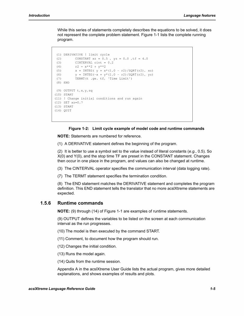
While this series of statements completely describes the equations to be solved, it does not represent the complete problem statement. Figure 1-1 lists the complete running program.
Figure 1-2: Limit cycle example of model code and runtime commands
NOTE: Statements are numbered for reference.
(1) A DERIVATIVE statement defines the beginning of the program.
(2) It is better to use a symbol set to the value instead of literal constants (e.g., 0.5). So X(0) and Y(0), and the stop time TF are preset in the CONSTANT statement. Changes then occur in one place in the program, and values can also be changed at runtime.
(3) The CINTERVAL operator specifies the communication interval (data logging rate).
(7) The TERMT statement specifies the termination condition.
(8) The END statement matches the DERIVATIVE statement and completes the program definition. This END statement tells the translator that no more acslXtreme statements are expected.
1.5.6 Runtime commandsNOTE: (9) through (14) of Figure 1-1 are examples of runtime statements.
(9) OUTPUT defines the variables to be listed on the screen at each communication interval as the run progresses.
(10) The model is then executed by the command START.
(11) Comment, to document how the program should run.
(12) Changes the initial condition.
(13) Runs the model again.
(14) Quits from the runtime session.
Appendix A in the acslXtreme User Guide lists the actual program, gives more detailed explanations, and shows examples of results and plots.
(1) DERIVATIVE ! limit cycle (2) CONSTANT xz = 0.5 , yz = 0.0 ,tf = 4.0 (3) CINTERVAL cint = 0.2 (4) r2 = x**2 + y**2 (5) x = INTEG( y + x*(1.0 - r2)/SQRT(r2), xz) (6) y = INTEG(-x + y*(1.0 - r2)/SQRT(r2), yz) (7) TERMT(t .ge. tf, ‘Time Limit’) (8) END
(9) OUTPUT t,x,y,sq(10) START(11) ! Change initial conditions and run again(12) SET xz=0.7(13) START(14) QUIT
acslXtreme Language Reference Guide 1-5

Introduction Coding procedure
1.6 Coding procedureThe acslXtreme coding line contains eighty columns and acslXtreme statements may be placed anywhere on the line. Standardized placement helps make programs easier to read.
1.6.1 Separator More than one statement can be placed on one line by separating the statements with a semicolon (;).
1.6.2 Continuation Any statement can becontinued on the next line by adding an ampersand (&) at the end of the line, to the right of any nonblank information but before column 80. Trailing blanks are removed from the line containing the ampersand and the following line is added directly. Starting with column 1, it is as though the characters were strung on the end after the last nonblank character of the preceding line. Leading blanks of the continuation line are not suppressed unless a leading ampersand is present on the continuation line. Comments can be added after the trailing ampersand since comments are stripped off first. An empty line needs two ampersands because a single one can’t be distinguished.
1.6.3 Comments Everything after an exclamation point (!) is considered a comment and ignored by the program translator and the runtime executive (in runtime commands).
1.6.4 Blank lines Blank lines can be placed anywhere in the program and have no effect.
1.7 Reserved namesThe only reserved names in the language are those of the form Znnnnn and ZZaaaa, where n is any digit and a is any alphanumeric character. All generated variables and system subroutine names are in this form.
1.7.1 System variable defaultsSystem variable default names are listed in Figure 1-3. These default names can be changed to any name, but if names are not specified, the default names exist so they can be set by program control in the model definition section.
1-6 acslXtreme Language Reference Guide

Introduction Reserved names
NOTE: Other uses of these names (e.g., defining MAXT as a state variable) could cause conflicts.
Figure 1-3: System Variable Default Names
1.7.2 Precedence of namesSymbols in SET commands are searched for first in the dictionary of acslXtreme system symbols. However, if a system symbol is used as a name in the program, it takes precedence over the acslXtreme system symbol. Generally duplicating system symbol names within the program interferes with the ability to modify system default values.
Statement Default name Default value Definition
ALGORITHM IALG 5 Integration algorithm
CINTERVAL CINT 0.1 Communication interval
ERRTAG none .FALSE. Error flag
MAXTERVAL MAXT 1.0E+10 Maximum calculation interval
MINTERVAL MINT 1.0E-10 Minimum calculation interval
VARIABLE T 0.0 Independent variable
acslXtreme Language Reference Guide 1-7

Introduction Reserved names
1-8 acslXtreme Language Reference Guide
Language Elements Introduction
Chapter 2 Language Elements
2.1 IntroductionFigure 2-1 lists the major points of the acslXtreme language . .
Figure 2-1: Main acslXtreme Syntax
2.2 ConstantsConstants may be integer, floating point (single or double precision), logical, or character. It is better to assign constants to variable names (see “Variables” ). Literal constants can be used in the source code, but their values can not be changed at runtime. To change a literal constant, all occurrences in the source code must be changed and the program retranslated, compiled, and linked. It is better to give all constants symbolic names via CONSTANT statements; i.e., rather than:
area = 3.142*r**2
the following code is preferred:
CONSTANT pi = 3.142
area = pi*r**2
2.2.1 Integer An integer constant is a whole number, written without a decimal point, exponent, or embedded blanks. Positive numbers may be prefixed with a plus sign; negative numbers
coding Free format; use any columns 1 through 80.
labels Labels can be alphanumeric. Labels are separated from the their statements by a colon; i.e., label: statement. Due to conflicts with macro expansions within labeled statements, labels should only be used with CONTINUE statements. See the section on labels.
names Name length is limited by the target language compiler. Names should not be of the form Znnnnn or ZZaaaa where n is any number and a is any alphanumeric character. Blanks are not allowed within names.
types All variables and functions are considered floating point (single or double precision depending on the library specified) unless typed explicitly otherwise.
continuation An ampersand (&) at the end of a line indicates continuation onto the next line.
comments An exclamation point (!) indicates a comment. acslXtreme ignores all code from an exclamation point to the end of the line.
acslXtreme Language Reference Guide 2-1
Language Elements Constants
must be prefixed with a minus sign. The maximum length of an integer is machine dependent. Subscripts of arrays are generally limited to five digits. Examples of integer constants include:
0 +526 -63 476
2.2.2 Promotion of integersA number without a decimal point (1 instead of 1.0) can normally be used where a floating point number is expected. The number is floated before it is used. However, a decimal point (or a variable name) should be used in arguments to functions, macros, or subroutines.
2.2.3 Floating point A floating point constant is written with a decimal point and/or an exponent. Positive numbers may be prefixed with a plus sign; negative numbers must be prefixed with a minus sign. The exponential forms are E (single precision) and D (double precision). Examples of floating point constants include:
3.1416 31.416E-1 7.9566314D-4 3E1
0.000345 0.347E03 -27.6E+220
Numbers entered with a decimal point and no exponent (e.g., 1.234) are given a double precision exponent of D0 (e.g., 1.234D0) when the global double precision translator option is selected. Numbers in expressions such as:
x = y*1.234
are handled by the compiler; i.e., the constant 1.234 is automatically promoted to double precision if y is double precision. However, since 1.234 is not an exact binary number, it is not as precise as 1.234D0. This promotion feature is primarily used in arguments to subroutines where it is impossible for the compiler to determine the precision of the subroutine argument when used inside the routine.
Use care when mixing integers and floating point numbers in subroutine arguments because the type may change. For example:
CALL mysub(1, 1.234)
must have arguments that are an INTEGER and a REAL. To prevent a mismatch in this situation, use the exponent form or one of the type conversion functions DBLE or REAL. REAL(1.234) is always single precision, and DBLE(1.234) and 1.234D0 are always double precision, but 1.234E0 is changed to 1.234D0. To ensure that the second argument is always single precision use the form:
CALL mysub(1, REAL(1.234))
2.2.4 Logical Logical constants may be one of two values.
.TRUE. .FALSE.
However, when logicals are plotted in acslXtreme, zero corresponds to .FALSE. and one to .TRUE.
2-2 acslXtreme Language Reference Guide
Language Elements Variables
2.2.5 Character Character constants are strings of letters, numbers, and other characters and are defined by placing them in single quotes. Single quotes can be inserted by doubling them; for example, to define a string abc’def, use ‘abc’’def’.
SET TITLE = ‘Limit Cycle, Run1’
2.3 VariablesVariable names are symbolic representations, usually for numerical quantities, that may or may not change during a simulation run. They refer to a location and the value is equal to the current number stored in that location. Both simple and subscripted variables may be used. Generally, variable name must start with a letter and be followed by up to thirty letters and digits, but this is limited only by the target language compiler. Underscores can be included in variable names to make them more readable.
this_long_name = INTEG(motor_velocity, initial_condition)
2.3.1 Types There are four types of variables: INTEGER, REAL, CHARACTER or LOGICAL. All acslXtreme program variables are assumed to be DOUBLEPRECISION (single or double precision, depending on the library specified) unless explicitly typed otherwise. Type REAL specifies single precision. only; Examples of simple variables include:
a a57 ab57 d k20
2.3.2 Subscripts A subscripted variable may have up to six subscripts enclosed in parentheses. Subscripts can be expressions in which the operands are simple integer variables and integer constants, and the operators are addition, subtraction, multiplication, and division only. For more information on storage allocation, see DIMENSION. Examples of subscripted variable names include:
b(5,2) b53(5*i + 2, 6, 7*k + 3)
c47(3) array(2) plate(2,2,3,3,2,2)
In the above examples, I and K must be declared explicitly to be INTEGER variables.
2.3.3 Array order Elements of arrays are written and accessed by column, then row; for example, the elements of b(2,5)can be shown:
11 12 13 14 15
21 22 23 24 25
Extracted as a single-dimensioned vector, the order is:
11 21 12 22 13 23 14 24 15 25
acslXtreme Language Reference Guide 2-3

Language Elements Labels
2.4 LabelsA label can be attached to a statement so that control is transferred to it by GOTO statement. Labels are alphanumeric. acslXtreme uses labels starting at 99999 and working downwards, therefore avoid labels with high numeric values to avoid possible conflicts.
2.4.1 Syntax A label is set off from the statement to which it applies by a colon (:), as in this example.
L1: CONTINUE
x = a + b 1000: y = c + d
GO TO L1
2.4.2 Statement labels and macro expansionAlthough statement labels can be attached to any executable statements, only CONTINUE statements are recommended. The difficulty is that the labeled statement may be translated into several statements; i.e., the effect of a macro call inside a statement is that the macro is expanded first, followed by the labeled statement.
For example, consider the random number generator GAUSS, which is a macro. It could be used in a labeled statement in a PROCEDURAL as follows:
GO TO label
...label: x = GAUSS(mean, sigma)
This expands to the Fortran code:
GO TO 99996
...
Z09999 = MEAN + GRV(ZZSEED)*(SIGMA)99996 X = Z09999
With the macro call in a labeled statement, the intermediate variable Z09999 is not assigned a value when the GO TO transition is executed. However, if a CONTINUE is used at the labeled statement as follows:
GO TO label
...
label: CONTINUEx = GAUSS(mean, sigma)
The code expands into the correct sequence as follows:
GO TO 99996
...
99996 CONTINUE
Z09999 = MEAN + GRV(ZZSEED)*(SIGMA) X = Z09999
2-4 acslXtreme Language Reference Guide

Language Elements Expressions
2.4.3 CONTINUE statements Attaching the LABEL to the first line of the code generated from the macro can work. However, DO loops become a problem, since the label must be the last operation of the loop (statements after the labeled statement are not in the loop). Even if acslXtreme differentiates between the DO loop labels, the language allows a loop with direct GO TOs to the terminating statement label; e.g.,
DO label i = 1, 20...
IF (condition) GO TO label
2.5 ExpressionsAn expression is a combination of operators and operands which, when evaluated, produces a single numerical value. Expressions may contain arithmetic, relational, and logical operators.
2.5.1 Arithmetic operatorsThe arithmetic operators are:
+addition
-subtraction
*multiplication/ division
** exponentiation
Two arithmetic operators can not appear next to each other in an arithmetic expression. If minus is to be used to indicate a negative operand, the sign and the element must be enclosed in parentheses if preceded by an operator; e.g.,
b*a/(-c) -a*b - c a*(-c)
are all valid, but the following is not:
b*a/-c
2.5.2 Parentheses Parentheses can be used to indicate groupings as in ordinary mathematical notation, but they cannot be used to indicate multiplication.
2.5.3 Warning – dividing by integerDividing by an integer (i.e., assuming that the integer is promoted to floating point) sometimes gives incorrect results. For example, the first calculation results in zero, but specifying the 2 in floating point gives the correct result:
x = 1/2/pi zero
x = 1/2.0/pi correct
ANSI standard forbids changing I/J/R to a supposedly equivalent I/(J*R). The following guidelines apply:
acslXtreme Language Reference Guide 2-5

Language Elements Expressions
1/2 integer zero1/2.0 floated to floating point
1/(2*pi) okay
1/pi/2 okay
2.5.4 Relational operatorsThe relational operators, the results of which can be only TRUE or FALSE, are:
.EQ.equal to
.NE.not equal to
.GT. greater than
.LT. less than
.GE.greater than or equal to
.LE. less than or equal to
2.5.5 Logical operatorsFigure 2-2 lists the Logical operators:
Figure 2-2: Logical Operators
2.5.6 Operands Operands may be constants, variables (simple or subscripted), or functions. Examples of arithmetic expressions include:
a 5.76 -(c + del*aero)
3 + 16.5 b + a(5)/2.75 (b - SQRT(a**2 + x**2))/2.0
Relational expressionsRelational expressions are a combination of two arithmetic expressions with a relational operator. The relational expression will have the value TRUE or FALSE depending on whether the stated relation is valid or not. The general form of the relational expression is:
a1 op a2
.EQV. combines two logical expressions to give the value TRUE when they are equivalent; otherwise, the value is FALSE
.NEQV. combines two logical expressions to give the value of TRUE when they are not equivalent and FALSE when they are equivalent.
.NOT. reverses the truth of the logical expression that follows it
.AND. combines two logical expressions to give the value TRUE when both are TRUE; otherwise, the value is FALSE
.OR. combines two logical expressions to give the value TRUE when either is TRUE; otherwise, the value is FALSE
2-6 acslXtreme Language Reference Guide

Language Elements Expressions
where ai are arithmetic expressions and op is a relational operator. A relational operator must have two operands combined with one operator. Examples of valid relational expressions include:
a .EQ. b a + d .LT. 5.3
a57 .GT. 0.0 5.0*b - 3.0) .LE. (4.0 - c)
Logical expressionsLogical expressions are combinations of logical operands and/or logical operators which, when evaluated, will have a value of TRUE or FALSE. The general form of the logical expression is:
l1 op l2 op 13 op ln
where li are logical operands or relational expressions. Examples are:
LOGICAL aa, cc, lfunc
aa .AND. (b .GE. c) .OR. cc .AND. lfunc(x,y) &
.AND. (x .LE. y) .OR..NOT. aa
NOTE: The symbolic names aa, cc, and lfunc have been declared to be of type LOGICAL, and lfunc is a function with a TRUE or FALSE result calculated from the value of the variables x and y.
Character expressionsCharacter constants and variables can be joined together by the // operator. Substrings of characters can be selected by a colon (:) operator; a substring may not be of zero length. For example:
c1 = c2(5:10)//c3
where c1, c2, and c3 are character variables. A character variable may not appear on both the left and right hand side of the same statement.
Mapping for the CHAR function depends on the character code used by the compiler. ASCII is almost universal. Integers can be converted to characters through the CHAR function; for example:
name = first//last//CHAR(period)
Single characters can be converted to integer (in the opposite direction to CHAR) by the ICHAR function.
Expressions in functionsArguments of functions may, in general, be expressions. Since expressions can contain functions, an arbitrary depth of complexity can be generated. Using the SIN and COS function as an example, the following is a valid expression:
a + SIN(x*COS(5*x + y) - COS(a + z/SIN(5.3*c) &
c*y/SIN(SIN(x + y)*pi)))
The sole requirement for an expression is that it have only one value when evaluated numerically.
acslXtreme Language Reference Guide 2-7

Language Elements Expressions
2-8 acslXtreme Language Reference Guide

Program Structure Implicit and explicit structure
Chapter 3 Program Structure
3.1 Implicit and explicit structureAn acslXtreme simulation model can contain only PROGRAM and END statements to outline the model structure. This is known as implicit structure because it implies that the whole program is a DERIVATIVE section. This simple structure has limitations, especially in handling initial conditions.
The more flexible explicit structure includes INITIAL, DYNAMIC (with embedded DERIVATIVE and DISCRETE), and TERMINAL sections, as shown in Figure 3-1. If this method is chosen, any or all of the five explicit blocks may be included. The order of the sections must be as shown, and each section must be terminated with its own END statement.
Figure 3-1: Outline of Explicitly Structured Program
PROGRAM
INITIAL
Statements executed before the run beings.State variables do not contain the initial conditions yet.
END
DYNAMIC
DERIVATIVE
Statements to be integrated continuously.
END
DISCRETE
Statements executed at discrete points in time.
END
Statements executed each communication interval.
END
TERMINAL
Statements executed after the run terminates.
END
END
acslXtreme Language Reference Guide 3-1

Program Structure Program flow
3.2 Program flowFigure 3-2 outlines the flow of an acslXtreme program with explicit structure. A program is activated with a runtime START command
Figure 3-2: Main Program Loop of acslxtreme Model
3-2 acslXtreme Language Reference Guide
Program Structure Program flow
3.2.1 INITIAL The program proceeds sequentially through the INITIAL section, the section for calculations performed once before the dynamic model begins. Initial condition values are moved to the state variables (outputs of integrators) at the end of the INITIAL section, but not all initial conditions will have been defined. Usually some initial conditions are calculated at this point. Any variables that do not change their values during a run can be computed in INITIAL. However, CONSTANT statements are not required to be placed in the INITIAL section; they are not executable and can be placed anywhere in the program.
3.2.2 DERIVATIVE DISCRETEThe integration routine is initialized when control transfers out of the INITIAL section. To ensure that all calculated variables are known before recording the first data point, the initialization procedure involves transferring all initial condition values into the corresponding states and evaluating the code in the DERIVATIVE and DISCRETE sections once.
NOTE: It may appear from the program listing that the DYNAMIC section is executed before the DERIVATIVE section; in fact, DERIVATIVE and DISCRETE are evaluated first and should not rely on calculations in the DYNAMIC section to initialize variables for DERIVATIVE or DISCRETE sections. On the other hand, all values calculated in the DERIVATIVE and DISCRETE sections are available in the DYNAMIC section.
3.2.3 DYNAMIC After initialization and evaluation of the DERIVATIVE and DISCRETE code, the STOP flag is reset and the program executes the code within the DYNAMIC block. There are no restrictions on the variables that can be referred to in this DYNAMIC section. All the states have values, and intermediate calculations in the DERIVATIVE and DISCRETE sections have been executed.
3.2.4 STOP flagAfter the DYNAMIC section has been evaluated, the STOP flag is tested; if the flag has been set, control is transferred to the TERMINAL region. The STOP flag is set by the TERMT statement; if any TERMT statements are included in the DYNAMIC block, control is transferred at this check when one of the arguments of TERMT becomes true. If the STOP flag has not been set, the program writes out the values of all the variables specified in the OUTPUT and PREPARE lists, the former to the output file or terminal, the latter to a scratch file for later plotting and/or printing.
3.2.5 Integration The integration routine is now asked to integrate over a communication interval (or until a termination condition is met) using the code embedded in the DERIVATIVE blocks to evaluate the state variable derivatives.
The integration routine returns with the states advanced through the communication interval and again the STOP flag is tested. At this point, the flag may have been set by a TERMT statement in a DERIVATIVE or DISCRETE section; if not, the program loops and re-executes the DYNAMIC section.
acslXtreme Language Reference Guide 3-3

Program Structure Program sorting
3.2.6 Transfer controlControl can be transferred between some sections using GO TOs and statement labels, if needed. It is illegal to transfer into the DYNAMIC region, since the integration initialization then could not be performed correctly. Transfer from the dynamic region to either INITIAL or TERMINAL is quite acceptable; so also is transfer between INITIAL and TERMINAL blocks. Control cannot be transferred either into or out of DERIVATIVE or DISCRETE sections since these are changed into a separate subroutine and, as such, are inaccessible to the main program loop.
3.2.7 TERMINAL Program control transfers to the TERMINAL section when the STOP flag has been set TRUE. On passing out of the last END, control returns to the acslXtreme executive, which reads and processes any further runtime commands (PLOT, DISPLAY, etc.). Note that if a jump (GO TO) sends control from the TERMINAL section back to the INITIAL, the last output is not written out unless the LOGD operator is used (see Chapter 4).
3.3 Program sortingThe acslXtreme translator sorts the code in the DERIVATIVE section so that outputs are calculated before they are used. Normal statements are sorted individually; PROCEDURAL sections are sorted as a unit based on the declared inputs and outputs, and no sorting is performed within the PROCEDURAL. Sorting takes place only within sections, never across sections. The sort algorithm is relatively simple and consists of two passes.
• Pass number one—examines each statement; output variables are marked as calculated and an input variable list consisting of all variables on the right of the equal sign is established for the statement. A variable name may appear simultaneously on both left and right hand sides of an equal sign in either an assignment statement or PROCEDURAL header. In this case, sorting takes place only on the left hand or output variable so that the block is positioned before any use of the variable.
• Pass number two—examines the list of statements one at a time. If, for a particular statement, none of the variables on the input variable list have their calculated flags set (meaning that the variable has already been calculated), the statement is added to the output statement list and the calculated flag for the output variable (or variables) is turned off. If any variables on the input variable list are marked calculated, the statement is placed in a temporary “saved” list and the next statement examined. If any statement has been added to the output statement list, all the saved statements are re-examined to see if they can now be added to the output statement list and their output variables reset. This algorithm works because any output variables that have already been processed have their calculated flags reset. Only output variables appearing later in the program are flagged and as such can hold up statements that depend on these outputs.
3.3.1 States State variables are not flagged as calculated. States are calculated by the integration routine before all derivative evaluations.
3-4 acslXtreme Language Reference Guide

Program Structure Proram Structure Preset of User Variables
3.3.2 CONSTANT For code readability, CONSTANT statements may be placed where they are used, thought it is recommended that constants be defined prior to their frst use.
3.4 Proram Structure Preset of User Variables
3.4.1 Algebraic loopsAlgebraic loops are identified during translation by the fact that statements are left over at the end of the DERIVATIVE section sort. This is considered an error since true algebraic loops should be broken by calculations, PROCEDURALs, or the implicit integrators IMPLC (scalars) or IMPVC (vectors).
Most algebraic loops are errors caused by incorrect PROCEDURAL headers or missing state equations. For example, the following code:
PROCEDURAL (a, b = c, d)a = c
b = d
END ! of procedurald = a
causes an algebraic loop to be reported since it implies that a is a function of both c and d, although this is not actually the case. Use PROCEDURALs sparingly and with care. Using many small PROCEDURALs is better than using a few large ones.
3.4.2 Diagnosing loopsWhen an algebraic loop is diagnosed, first check the PROCEDURALs for errors. Second, check for a modelling error such as a missing state in a control loop.
3.4.3 Multiple INITIAL, DYNAMIC, and TERMINAL sectionsINITIAL sections and TERMINAL sections can be placed anywhere in a program. The translator appends each INITIAL section to the end of any collected previously (to a default null INITIAL if there is no explicit user INITIAL before the DYNAMIC or DERIVATIVE). Similarly, TERMINAL sections are collected as the translator sorts through the program, each appended to any collected previously. Thus, any TERMINAL sections defined in a DERIVATIVE section, for example, occur before the code in an explicit final TERMINAL section.
3.4.4 Section nestingAny section (INITIAL, DYNAMIC, DERIVATIVE, DISCRETE, or TERMINAL) can be nested within any other section, to any level of nesting. For example, in a DERIVATIVE section, one can write:
SCHEDULE burnout .XN. acceleration
DISCRETE burnout
INITIAL; dt = GAUSS(0.050, 0.001); END
SCHEDULE separation .AT. t + dtEND ! of burnout
acslXtreme Language Reference Guide 3-5
Program Structure Preset of user variables
3.5 Preset of user variablesThe acslXtreme executive presets all floating point variables to 5.5555E33, integers to 55555333, and logicals to .FALSE. This helps prevent unknowingly using wrong values if the variable is used before it is calculated, particularly where a value of zero would allow the program to proceed when it should not.
NOTE: When variables are not calculated before being used and where more than one START is executed in a runtime session, all runs after the first use values left at the end of the previous run. Setting all user variables to a large number aids in identifying uncalculated variables in the first debugging runs.
3.6 Preset of derivativesThe acslXtreme executive presets all derivatives and residuals (as defined in INTEG, INTVC, IMPLC, and IMPVC statements) before each START to 3.33333333E-33. After the initial evaluation of the DERIVATIVE section, the executive checks that all derivatives have changed from the preset value; if not, an error message is produced:
DERIVATIVE NO. n NOT CALCULATED
This message usually indicates that a derivative calculation has been skipped or that a derivative is specified with a CONSTANT statement, which is not executable. Determine which derivative is referenced in the message by checking a DEBUG dump or DISPLAY/ALL and counting down the list of derivatives.
3-6 acslXtreme Language Reference Guide

acslXtreme Statements Introduction
Chapter 4 acslXtreme Statements
4.1 IntroductionThis chapter describes in detail all the basic statements recognized by the acslXtreme translator.
acslXtreme places no restriction on column placement of the code. The generic form of functions is recommended; e.g., use ABS instead of IABS, DABS, or CABS and MAX instead of AMAX0, AMAX1, MAX0, MAX1, DMAX0, or DMAX1. To specify a typed (non-generic) function reduces flexibility, while the generic functions adapt to single or double precision, INTEGER or REAL type, automatically.
4.1.1 Documentation conventionIn the following examples and descriptions, elements in lower case are syntactical elements (i.e., variables) and may be replaced with any character string that satisfies the definition. Elements shown in upper case must be exactly as spelled out in the statement (although not necessarily in upper case). In specifying the integration operator, for example, the word INTEG must be given exactly while all the other elements are variables you name as part of the model. The form is specified as:
state = INTEG(deriv, ic)
An example would then be in the form:x = INTEG(xd, xic)
4.1.2 ! & ; : The use of these characters in program code is described in this chapter under Comment (!), Continuation (&), and Separator (;). The ampersand (&) is also used for concatenation in macros (see Chapter 5). Statement labels, using a colon (:), are discussed in Chapter 2. Wild cards (* and ?) are available for many of the runtime commands, but are not used in program code.
4.1.3 CONSTANT recomputationVariables defined in CONSTANT statements generally should not also be defined in assignment statements. If the translator encounters this situation, it issues the following warning message:
Warning: Re-computing a constant
acslXtreme Language Reference Guide 4-1
acslXtreme Statements Introduction
See the section on CONSTANT in this chapter. The warning message can be suppressed.
4.1.4 Debugging Calls to LOGD can help debug a program when a system debugger is not available. See LOGD in this chapter for a description of this procedure.
4.1.5 Equal sign (=) acslXtreme uses the equal sign in an unfamiliar way. In translating a program, acslXtreme needs to know the each statement’s inputs and outputs so that the statement sequence can be sorted into the correct order. In assignment statements, all variables to the right of the equal sign are inputs; the variable to the left is given the single numerical value of the right hand expression and thus is the output. This concept is extended to cases where more than one element is an output; i.e., all elements to the left of the equal sign are considered outputs and those to the right are considered inputs.
4.1.6 Equal sign in PROCEDURALThis concept of the use of equal signs is extended to the PROCEDURAL, which has the following possible form:
PROCEDURAL(a, b, c = d, e)
... block of statements
END
This code tells the translator to treat the statements bracketed by the PROCEDURAL and its matching END statement as a block (i.e., not to rearrange the order within the block); that D and E are inputs; and that A, B, and C are outputs. Only variables calculated elsewhere in the same DERIVATIVE section must be listed on the input list. Constants need not appear on the list. State variables (output of state operators) must not appear on the list.
See the PROCEDURAL section in this chapter for details on when and how to use this structure. See Chapter 3 for information on program flow and statement sorting.
4.1.7 Operators for simulation modelsThis chapter includes descriptions of several functions especially designed for simulation models. In general, the output of each function is a single number (usually floating point) and the arguments are arithmetic expressions of arbitrary complexity; i.e., these expressions may contain functions which contain arguments which contain functions to any depth.
4-2 acslXtreme Language Reference Guide
acslXtreme Statements Introduction
Logical or relational expressions are used to determine switching criteria in the special functions. Only .TRUE. or .FALSE. are used for logical constants. Other logical representations may not be recognized because the bit pattern of logicals depends on the installation and compiler in use.
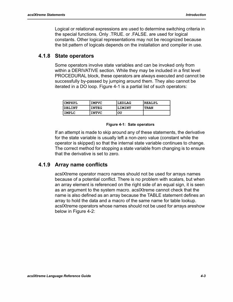
4.1.8 State operators Some operators involve state variables and can be invoked only from within a DERIVATIVE section. While they may be included in a first level PROCEDURAL block, these operators are always executed and cannot be successfully by-passed by jumping around them. They also cannot be iterated in a DO loop. Figure 4-1 is a partial list of such operators:
Figure 4-1: Sate operators
If an attempt is made to skip around any of these statements, the derivative for the state variable is usually left a non-zero value (constant while the operator is skipped) so that the internal state variable continues to change. The correct method for stopping a state variable from changing is to ensure that the derivative is set to zero.
4.1.9 Array name conflictsacslXtreme operator macro names should not be used for arrays names because of a potential conflict. There is no problem with scalars, but when an array element is referenced on the right side of an equal sign, it is seen as an argument to the system macro. acslXtreme cannot check that the name is also defined as an array because the TABLE statement defines an array to hold the data and a macro of the same name for table lookup. acslXtreme operators whose names should not be used for arrays areshow below in Figure 4-2:
CMPXPL IMPVC LEDLAG REALPLDBLINT INTEG LIMINT TRANIMPLC INTVC OU
acslXtreme Language Reference Guide 4-3

acslXtreme Statements Introduction
Figure 4-2: acslXtreme operators that should not be used for arrays
4.1.10 Standalone form of operatorsSome operators are defined as macros. When the operator has only one output, two alternative forms of invocation (conventional and standalone) are possible. For example, consider the conventional use of REALPL, the first order lag:
y = k1*REALPL(t1, x)
The state variable (output of the real pole function) is given a dummy name (a Z variable). It usually helps to multiply the input rather than the output by constants (synonymous if the operator is linear) as follows:
y = REALPL(t1, k1*x)
Now the input to the operator is an expression and in this form the standalone macro invocation can be used as follows:
REALPL(y = t1, k1*x)
In this case (only) the variable y is assigned to the state table. This standalone form is usually preferred to minimize the number of dummy variables, and still all forms are numerically equivalent.
Operators that can be given in standalone form are noted in their individual descriptions. They are listed below in Figure 4-3 :
Figure 4-3: Operators that can be given in standalone form
BCKLSH IMPL OU RSHM WDACCMPXPL IMPLC OUTPUT RSHMI WDACFDBLINT IMPVC PREPAR RTDEVICE WDIGDELAY INTEG PTR RTP WDZGIDELAYP INTVC RADC SCALE WSHMDELSC LEDLAG RADCI SMOOTH WSHMIZOHDELVC LIMINT RDIG TERMTDERIVT LIMIT RDIGI TRANGAUSI LINEAR REALPL TRANZGAUSS LINES RESET UNIFHISTORY MODINT RSHM UNIFI
BCKLSH DELSC LEDLAG REALPLCMPXPL DELVC LIMINT SMOOTHDBLINT GAUSS LINEAR TRANDELAY HISTORY OU UNIF
4-4 acslXtreme Language Reference Guide
acslXtreme Statements ABS
4.1.11 Precision of acslXtreme operatorsBy default, the precision of operators in acslXtreme is DOUBLEPRECISION.
4.1.12 Forcing precision Forcing precision is usually necessary only if a variable is to be an argument to an external subroutine within which a particular precision is specified. Assume a subroutine MYSUB with two scalar real arguments, one scalar double and one vector double precision arguments; i.e.,
CALL mysub(rs1, rs2, ds1, dv2)
Then types would be specified as follows to ensure consistency within the subroutine:
REAL rs1,rs2
DOUBLEPRECISION ds1,dv2(20)
Another approach is to use the generic type changing functions REAL( ) and DBL( ) for the scalars. Then the type has to be specified only for the vector as follows:
DOUBLEPRECISION dv2(20)
CALL mysub(REAL(rs1), REAL(rs2), DBLE(ds1), dv2)
This is the preferred way since the actual precision of the variables RS1, RS2, and DV1 is immaterial in the acslXtreme program.
4.2 ABS
Form: y = ABS(x)
Description:
The output y is the absolute value of x where x is an expression. The output type (INTEGER, or REAL, DOUBLEPRECISION) depends on the input type.
Example:cd = cdz + cdal*al + cdde*ABS(dle)
4.3 ACOS
Form: y = ACOS(x)
acslXtreme Language Reference Guide 4-5

acslXtreme Statements AINT
Description:
The output y is the arc cosine of x where x is a floating point variable or expression lying between -1.0 and +1.0. The result, in radians, lies between zero and p. The result type (REAL or DOUBLEPRECISION) depends on the input type.
Example:th = ACOS(x/r)
4.4 AINT
Form:y = AINT(x)
Description:
The output y is the truncation of x where x is a floating point variable or expression. The output type (REAL or DOUBLEPRECISION) depends on the input type. This function differs from INT where the output is type INTEGER for any type input. In the following example, the result is -3.0.
a = AINT(-3.7)
Since INT( ) is promoted to REAL or DOUBLE as appropriate in any expression, the only situation where it is necessary to use AINT( ) is in the argument to a subroutine in order to force the type.
Example:
If the first argument of MYSUB is floating point, the following ensures a truncated (integer) value, but transmitted as a floating point number:
CALL mysub(AINT(v1), ...)
Using INT( ) in this situation doesn’t work since the argument is passed with type integer.
4.5 ALGORITHM
Form:ALGORITHM name = integer constant
Default:name:IALG
integer constants: 5
4-6 acslXtreme Language Reference Guide

acslXtreme Statements ALGORITHM
Description:
Where name is the new name for the integer defining the runtime algorithm. This statement can change the system variable name and/or the choice of integration routine. The name IALG is the default and its value may be set numerically at runtime even if the ALGORITHM statement has not been specified in the program.
4.5.1 Array with multiple sections
Description:
If a program contains only one DERIVATIVE section and no DISCRETE sections, ALGORITHM name (referred to by its default name IALG hereafter) is a scalar. If the program has more than one DERIVATIVE and/or DISCRETE section then IALG becomes an array. The elements in IALG then correspond to the sections in the order they are encountered in the source code. If ALGORITHM is defined outside a DERIVATIVE section, then it is the global default for all DERIVATIVE sections. DISCRETE sections have their algorithm slot set automatically zero. To change the algorithm for a specific DERIVATIVE section, put an ALGORITHM statement with a unique name in the section.
Example:DERIVATIVE
ALGORITHM fastalg = 4
The scalar name given is equivalenced to the array element; for example, if the DERIVATIVE section is first in the program, FASTALG is equivalenced to IALG(1). At runtime, either the array element or the local name can be referenced.
SET IALG(1)=1SET fastalg=8
NOTE: Do not change during run. The choice of integration algorithm cannot be changed during a run because table space has to be allocated before the run begins. After acslXtreme determines the IALG for a run, it does not look again to see if it has changed. The communication interval and/or integration step size can be changed.
4.5.2 Recommended integration control
Description:
Figure 4-4 lists the available integration algorithms. For fixed step algorithms, we recommend setting NSTEPS (NSTP) to 1 so that you control the step size with MAXTERVAL (MAXT) and the data logging rate
acslXtreme Language Reference Guide 4-7

acslXtreme Statements ALGORITHM
with the communication interval CINTERVAL (CINT). The integration step size for fixed step algorithms is calculated by:
H = MIN(MAXT, CINT/NSTP)H = MIN(H, time_to_next_event)
CINT is divided by NSTP. If NSTP is 1 and MAXT is less than CINT, then MAXT sets the integration step size and CINT affects only the data logging rate. Events include DISCRETE sections (usually controlled by an INTERVAL statement), state events or time events activated by SCHEDULE statements, and CINT. CINT does not have to be an even multiple of MAXT since the integration steps up to it automatically.
Figure 4-4: Avaliable Integraion Algorithms
4.5.3 Fixed step algorithms
Description:
The Runge-Kutta routines (IALG = 4 and 5) evaluate the derivatives at various points across a step. A weighted combination of these derivatives is then used to step across the interval. Euler (IALG=3) makes just one derivative evaluation and the step size must be small compared to that of other algorithms to achieve acceptable accuracy. Euler is used for any integrations required by operators in DISCRETE sections. Runge-Kutta second order advances the state with two derivative evaluations per step. This usually needs a somewhat smaller step than Runge-Kutta fourth order (four derivative evaluations per step). For the same step size, it should run about twice as fast. Optimizing the step size and algorithm is generally worth the effort.
IALG Algorithm Step Order
1 Adams-Moulton variable variable
2 Gear’s stiff variable variable
3 Euler fixed first
4 Runge-Kutta fixed second
5 Runge-Kutta fixed fourth
6 none – –
7 user-supplied – –
8 Runge-Kutta-Fehlberg variable second
9 Runge-Kutta-Fehlberg variable fifth
10 Differential algebraic system solver
variable variable
4-8 acslXtreme Language Reference Guide

acslXtreme Statements ALGORITHM
4.5.4 Runge-Kutta procedure
Description:
Figure 4-5 shows the procedure for the fourth order Runge-Kutta algorithm. If x is the state, h is the integration step size, and t is time, the derivative k is evaluated at the beginning, twice at the midpoint, and once at the end of the integration step as follows:
The new state is then calculated by:
The second order Runge-Kutta routine follows a similar procedure, making one derivative evaluation at the beginning and another at a point two-thirds across the step as follows:
The new state is then weighted by one-fourth and three-fourths and calculated by:
MINT, XERROR, and MERROR (discussed below for the variable step algorithms) do not affect the fixed step algorithms in any way.
Figure 4-5: Runge-Kutta fourth order algorithm
k1 f xn tn,( ) =
k2 f xnhk12
-------- tnh2---+,+
=
k3 f xnhk22
-------- tnh2---+,+
=
k4 f xn hk3 tn h+,+( ) =
xn 1+ xnh6--- k1 2k2 2k3 k4+ + +( )+=
k1 f xn tn,( )
k2 f xn2hk1
3----------- tn
2h3
------+,+
=
=
xn 1+ xnh4--- k1 3k2+( )+=
acslXtreme Language Reference Guide 4-9

acslXtreme Statements ALGORITHM
4.5.5 Variable step algorithms
Description:
The Adams-Moulton (IALG=1) and Gear’s Stiff (IALG=2) are both variable step, variable order integration routines that are self-initializing. In general they attempt to minimize the step changing by always choosing a step size that divides evenly into the time-to-go to the next event and keeping the per-step error in each state variable below an allowed value. This desired value is obtained by taking the maximum of the corresponding absolute allowed error (XERROR) and the relative allowed error (MERROR) multiplied by the maximum absolute value of the state so far:
The order of integration starts at one and then changes dynamically as the program progresses. The step size also changes dynamically as the integration routine attempts to take the largest possible step consistent with the allowed error bounds.1
4.5.6 Adams-Moulton
Description:
Adams-Moulton is useful for models in which the step size changes significantly during a simulation, as for a satellite in a highly eccentric orbit. In this case, a much larger step size can be used when the satellite is far from the earth than when it is near. This algorithm can also help determine an appropriate step size for fixed step runs, as described below.
4.5.7 Gear’s stiff
Description:
Gear’s algorithm is for stiff systems that have frequencies of three or four orders of magnitude difference, where the high frequency motions are extremely active at some point (such as in a chemical reaction, explosion, etc.) and then smooth to essentially zero amplitude. The Gear’s stiff algorithm is then able to take large time steps since only the low frequency motions are of interest.
Gear’s stiff integration can take steps that are orders of magnitude larger than the smallest time constant in a stiff system. There is an overhead involved, however, since a linearized state transition matrix must be formed
1. For more information on mechanization of the variable step, variable order integration rou-tines, see subroutine DIFSUB in Numerical Initial Value in Ordinary Differential Equations, C.W. Gear, Prentice-Hall, NJ 1971 pp 150 et seq.
Ei MAX Xi Mi∗ Yi MAX,( )=
4-10 acslXtreme Language Reference Guide
acslXtreme Statements ALGORITHM
and inverted. Tests have shown that for problems where the range of time constants differs by only one or two decades, there is little benefit in using this method; Adams-Moulton is invariably faster. If the range of time constants covers more than three or four decades, then this technique may be significantly faster than any other.
4.5.8 Runge-Kutta-Fehlberg
Description:
The Runge-Kutta-Fehlberg algorithms (IALG = 8, 9) are fixed order but variable step. They are useful for models with a number of discontinuities, such as a system in which a spring is encountered periodically. The Adams-Moulton method uses information from previous steps to determine the size of the current step, but the Runge-Kutta-Fehlberg method starts fresh each step, thus having less difficulty with discontinuities. These routines adjust the step length to keep the error per step less than that specified by XERROR and MERROR. The relative error (MERROR) values are applied to the largest absolute value of the state so far, not the current value.
Algorithm 8 evaluates the derivative three times per step and makes a second order state advance; algorithm 9 evaluates the derivative six times and makes a fifth order state advance. If any error in a state is larger than that allowed, the step size is reduced (by no more than 0.1 at a time) until the error criteria are satisfied for all states or the minimum step size (MINT) is reached. After a successful step, the new step size is set to be 0.8 (for IALG = 8) or 0.9 (for IALG = 9) of a step size which would result in the maximum allowable error (as calculated during the previous step), except that the new step size is not less than the previous successful one.
The lower order algorithm (IALG = 8) is recommended for most applications because it usually uses less computer time.
4.5.9 Differential algebraic system solver (DASSL)
Description:
The DASSL code1 (IALG of 10) is intended to directly solve implicit differential algebraic equations (DAEs) where the derivative term cannot be specifically isolated on the left hand side of an equation. In this case, instead of:
1. For more information on the mechanization of DASSL, see Numerical Solution of Initial Value Problems in Differential Algebraic Equations, by E.E. Brenan, S.L. Campbell, and L.R. Pet-zold, North-Holland, 1989.
Y· F Y t,( )=
acslXtreme Language Reference Guide 4-11

acslXtreme Statements ALGORITHM
we have:
where F, Y and are N-dimensional vectors and the zero is really the residual that is being driven to zero. The following introductory description is take from Brenan, Campbell, and Petzold p. 117. The basic idea for solving the DAE system using numerical ODE methods, originating with Gear, is to replace the derivative in the above equation by a difference approximation and then solve the resulting system for the solution at the current time using Newton’s method. Replacing the derivative by the first order backward difference, we obtain the explicit Euler formula:
where:
This nonlinear system is then solved for Yn+1 using a variant of Newton’s method. DASSL uses a fixed leading coefficient implementation of the BDF formula which can approximate the derivative to higher accuracy at higher orders. The advantage of the fixed leading coefficient is that this is the term that appears in the iteration matrix, and the matrix only has to be recalculated on a change of step size – not on every subsequent step – as the history washes out of the range of information needed to be saved by backward differences.
In acslXtreme, the implicit form:
is expressed as:y, yd = IMPLC(F(y,yd,t), yic)
and is really implemented by adding both y and yd to the state vector as:y = INTEG(yd, yic)
yd = IMPLC(F(y,yd,t), 0.0)
Thus, for every algebraic/differential state, two slots are allocated in the state table.
4.5.10 MINT with variable step algorithms
Description:
The variable step algorithms never take steps smaller than MINTERVAL (MINT). The integration step size for variable step algorithms is calculated as for the fixed step algorithms with the addition of a check on the minimum step size as follows:
F Y Y· t, ,( ) RESIDUAL 0= =
γ·
F Yn 1+ , Yn 1+ Yn–
hn 1+------------------------ tn 1+,
0=
hn 1+ 1n 1+ tn–=( )
F Y Y· t, ,( ) 0=
4-12 acslXtreme Language Reference Guide
acslXtreme Statements ALGORITHM
H = MAX(MINT, MIN(MAXT, CINT/NSTP))
4.5.11 NSTP with variable step algorithms
Description:
NSTP can be set to help a variable step algorithm start off. If the first try (CINT/NSTP) is too large (i.e., if the estimated error is larger than the allowed error), the algorithm reduces the step size and tries again, until it finds a small enough step size to start off. Setting NSTP to a fairly large number (1000, for example) starts the routine at small step size, which is then increased automatically as the run progresses until it reaches the most efficient size. Beware of leaving NSTP at a large value and switching to a fixed step algorithm.
4.5.12 Error summary
Description:
An error summary is produced automatically at the end of simulation runs using variable step algorithms, giving the weight each state had in controlling step size. The error criteria (XERROR and MERROR) can be adjusted using this information. The number of times the predictor-corrector algorithm failed to converge and caused a general step size reduction is also listed. This is usually considered a more serious failure than bumping into the allowable error tolerance. The summary may be suppressed by setting the system variable WESITG (write error summary, integration control) to FALSE. Current step size (CSSITG) and current integration order (CIOITG) are available as system variables that can be OUTPUT or PREPAREd.
4.5.13 Determining appropriate step size
Description:
Determining an appropriate step size for a fixed step algorithm is important. If a step size is too large, the results are inaccurate or even catastrophic; if too small, computer time is wasted.
One approach is to use a variable step algorithm to see what acslXtreme believes to be appropriate. Use the Adams-Moulton routine and the system variables for current step size and current integration order as follows:
SET IALG=1
PREPARE T,CSSITG,CIOITG ...START
PLOT CSSITG,CIOITG
acslXtreme Language Reference Guide 4-13
acslXtreme Statements ANINT
Check that the step size is not being constrained by CINT. If it is, increase CINT and MAXT and run the simulation again. Look at the shape of CSSITG. If it is steady, use a fixed step size just slightly larger than the values chosen by the variable algorithm (the system choice of step size is somewhat conservative, so a slightly larger step is usually adequate). If the curve varies widely, however, consider using one of the variable algorithms. The system choice of CIOITG should also be steady and can be factored into the choice of algorithm order and step size.
4.5.14 Efficiency and accuracy
Description:
The efficiency of the various algorithms can be compared with the SPARE command.
Example:SET IALG = 4
SPARE;START /nc;SPARESET IALG = 5
SPARE;START /nc;SPARE
Each SPARE command lists the cpu time elapsed since the previous SPARE command. Compare the accuracy of the results by printing (or plotting) significant variables or by getting debug dumps.
4.6 ANINT
Form: y = ANINT(x)
Description:
The output y is the nearest whole number of x where x is a floating point variable or expression. The output type (REAL or DOUBLEPRECISION) depends on the input type.
Since NINT is promoted to REAL or DOUBLE as appropriate in any expression, the only situation where it is necessary to use ANINT( ) is in the argument to a subroutine to force the type.
Example:
If the first argument of MYSUB is floating point, the following ensures the nearest whole number (integer) value, but transmitted as a floating point number:
CALL mysub(ANINT(v1), ...)
4-14 acslXtreme Language Reference Guide

acslXtreme Statements ASIN
4.7 ASIN
Form:y = ASIN(x)
Description:
The output y is the arc sine of x, where x is a floating point variable or expression between -1.0 and +1.0. The output is in radians (−π ⁄ 2 ≤ y ≤ + π⁄ 2 ); its type (REAL or DOUBLEPRECISION) depends on the type of the argument.
Example:
ASIN could be used as follows:area = 0.5*pi*r**2 - x*SQRT(r**2 - x**2) + (r**2)*ASIN(x/r))
4.8 Assignment statements
4.8.1 Arithmetic
Form:variable = expression
Description:
Where variable may be simple or subscripted. If a subscripted variable is used in a sorted section, it must be enclosed in a PROCEDURAL block. On execution, the single value of the expression is stored into the location defined by variable; for example, the results of the expression on the right side of the following statement is stored into location y:
y = a*b + c/d
A special form of the assignment statement is the integration statement. The use of the INTEG operator marks the variable as a state variable.
Example:
In this example, a is marked as a state variable and ad is stored as the derivative of A.
a = INTEG(ad, aic)
Type conversion is performed automatically from an integer, real, or double precision expression to an integer, real, or double precision variable.
acslXtreme Language Reference Guide 4-15
acslXtreme Statements ATAN
4.8.2 Logical
Form:lvariable = lexpression
Description:
where lvariable may be simple or subscripted and lexpression is a logical expression formed from a logical operator.
Example:flag = a .NE. b .OR. flag2
4.8.3 Character
Form: cvariable = cexpression
Description:
where cvariable is a character variable or substring and cexpression is a character expression.
Example:cvar(5:10) = string(1:4)//’Z’
concatenates a Z to four characters extracted from STRING and places them in character positions 5 through 9. Unfilled character positions in cvariable are filled with blanks. If the length of cexpression exceeds that for cvariable, the character expression is truncated on the right.
4.9 ATAN
Form: y = ATAN(x)
Description:
The output y is the arc tangent of the floating point argument x where x is unlimited except for infinity and the result is in radians in the range (−π ⁄ 2 < y < +π⁄ 2 ).
Example:al = ATAN(-vmm(3)/vmm(1))
For full coverage of the circle, it is better to use ATAN2.
4-16 acslXtreme Language Reference Guide

acslXtreme Statements ATAN2
4.10 ATAN2
Form: z = ATAN2(y, x)
Description:
The output z is the arc tangent of an angle formed by the point with floating point coordinates x, y and the positive x-axis; x and y can be both positive and negative, defining the full circle of revolution. The result is in radians in the range (−π < z ≤ + π ).
Example:pdgn = ATAN2(dlq, dlp + 1.0E-30)
4.11 BCKLSH
Form:y = BCKLSH(ic, dl, x)
BCKLSH(y = ic, dl, x)
Description:ic = initial condition of ydl = half the width of the backlash
x = input (a floating point variable or expression)
The output always lies between the limits (x - dl) and (x + dl). Figure 4-6 illustrates the backlash mechanism.
Figure 4-6: Mechanism Illustrating BCKLSH Operator
For asymmetrical applications, the input x expression should be rewritten. For example, if y is to move when x is greater than (Y+UL) or less than (Y-LL), then:
y = BCKLSH(yic, 0.5*(ul - ll), x - 0.5*(ul + ll))
acslXtreme Language Reference Guide 4-17

acslXtreme Statements BOUND
NOTE: The BCKLSH operator must be in a sorted (DERIVATIVE) section.
4.12 BOUND
Form: y = BOUND(bb, tb, x)
Dscription:bb = bottom bound
tb = top bound
x = input (a floating point variable or expression)
The output y is as follows:y = bb when x < bb
y = x when bb < x < tb
y = tb when x > tb
This function bounds or limits variables. It should not be used to limit the output of an integrator since the integrator itself continues to wind up and must actually integrate out of the limit. The function LIMINT should be used in this case.
Example:MAXT = BOUND(maxtmn, maxtmx, maxtp)
4.13 CALL
Form:CALL name
CALL name (p1, p2, ..., pn)
CALL name (o1, o2, ..., on = p1, p2, ..., pn)
Description:
Where name is the name of a subroutine being called, pi are actual arguments that may be expressions of arbitrary complexity for input values, and oi are output variables (names or arrays). Arguments may be variables, arrays, or subscripted variables.
In the third form, the translator cannot tell which arguments are inputs and which are outputs. If the call is in a sortable section of the program, it should be embedded in a PROCEDURAL block that describes the inputs and outputs. If the call is any other section, a PROCEDURAL is recommended to avoid the “Symbol used but not defined” diagnostic.
4-18 acslXtreme Language Reference Guide

acslXtreme Statements CHARACTER
Example:
If oi are output variables and pi are input variables or expressions, then the following statements are valid:
PROCEDURAL (o1, o2, o3 = p1, p2, p3, p4)
CALL subr(o1, p1, p2, p3, p4, o3, o2)END
Now the translator sorts this section correctly since it has been told which variables are inputs and which are outputs.
The third form of the call is available for the case in which the subroutine is defined with the input expressions on the left and the output variables on the right. In this form, the subroutine could be called with:
CALL subr(o1, o2, o3 = p1, p2, p3)
The translator rearranges the order and changes the equal sign to a comma so that the resulting call to FORTRAN is:
CALL subr(p1, p2, p3, o1, o2, o3)
4.14 CHARACTERSee TYPE.
4.15 CINTERVAL
Form:CINTERVAL name = real constant
Default:name: CINT
real constant: 0.1
Description:
Where name is a simple unsubscripted variable.
The communication interval CINTERVAL is the interval at which the DYNAMIC section is executed and the variables on the OUTPUT and PREPARE lists have their values recorded. In general, no finer detail can be seen in OUTPUT, PRINT, or PLOT, so it is important to choose this value with care. A communication interval that generates about 100 to 200 data points during a run is sufficient detail for most applications.
acslXtreme Language Reference Guide 4-19

acslXtreme Statements CINTERVAL
Sampling effect
Be careful of the sampling effect where high frequency oscillations can be folded down to lower frequencies or even a DC level if the sampling time is not small enough.
4.15.1 Adjusting step size to CINTIf the next integration step to a communication interval is less than 1.0E-11 (1.0E-6 in single precision) of the current time (or CINT, whichever is larger), the step is discarded as negligible. This situation can occur because of accumulation and rounding on a binary machine. The integration algorithm takes steps up to the next communication interval by accumulating the fixed step (for example, with MAXT = 0.01and CINT = 0.1; after ten steps, the time is about 0.1 because of rounding in both 0.01 and 0.1). To prevent accumulated round-off error, a small adjustment is made to the communication interval. CINT is multiplied by a power of ten until it is close to an integer, then time is accumulated as an integer but divided by the multiplier before being used.
4.15.2 Double precision To get full precision when changing CINT and MAXT at runtime, use the double precision specification:
SET cint = 0.1D0
SET maxt = 0.01D0
4.15.3 Calculating CINT The value of the name defined in the CINTERVAL statement can be calculated in the program so that different phases can be viewed at different data rates. For example, assume that a missile simulation has the following four phases of flight:
1)Initial turn
2)Midcourse
3)Acquisition4)Terminal
It is useful to measure these phases at different rates; e.g., initial turn at a fairly fine level of 0.1 second, the long midcourse only every second, and acquisition and terminal at a fine rate of 50 msec. Figure 4-7 outlines a procedure for setting the communication interval for each phase. In the INITIAL section, PHASE is declared to be an integer and initialized to one. An array CINTTAB is defined and filled with the communication intervals to match the phases of flight as numbered above. In the DYNAMIC section, the communication interval (using default name CINT) is set using the
4-20 acslXtreme Language Reference Guide

acslXtreme Statements CINTERVAL
current value of the flight PHASE (which ranges from one to four). In the DERIVATIVE section, the value of PHASE is computed from the logic used to establish the different flight regions. This code is shown as a block since the algorithm depends on the implementation of the model; but no matter how it is implemented, the value of PHASE is maintained in the range one to four.
INITIAL
INTEGER phase
DIMENSION cinttab(4)CONSTANT cinttab = 0.1, 1.0, 0.05, 0.05
phase = 1 ! Initialize phase to start
...END ! of initial
DYNAMIC
DERIVATIVE! Compute phase of flight
PROCEDURAL(phase = , , ... )
...END ! of procedural
...
END ! of derivativeCINT = cinttab(phase)
...
END ! of dynamic
Figure 4-7: Outline of program to vary communication interval Changing default
4.15.4 Changing default nameThe name of the variable defining the communication interval can be changed from the default CINT;
Example:CINTERVAL CI = 0.001
Now all references are to CI when the value is recorded or changed.
4.15.5 Bound on integration stepCINTERVAL acts as an upper bound on the integration step size (and also for the last integration step of a communication interval) since the model is advanced no further than to the data recording time no matter how large the calculated integration step size. This subject is discussed in more depth under DYNAMIC. The actual integration step is obtained from the following algorithm:
H = MIN(MAXT, CINT/NSTP)
H = MIN(H, time_to_next_event)
acslXtreme Language Reference Guide 4-21
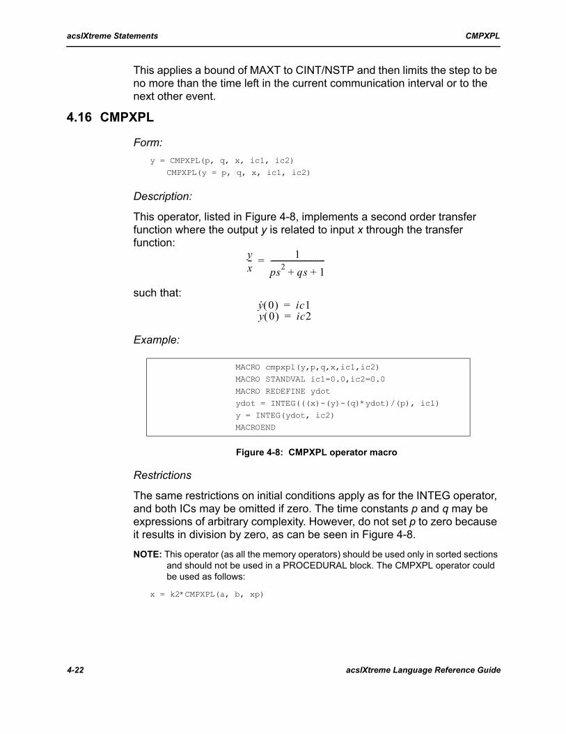
acslXtreme Statements CMPXPL
This applies a bound of MAXT to CINT/NSTP and then limits the step to be no more than the time left in the current communication interval or to the next other event.
4.16 CMPXPL
Form:y = CMPXPL(p, q, x, ic1, ic2)
CMPXPL(y = p, q, x, ic1, ic2)
Description:
This operator, listed in Figure 4-8, implements a second order transfer function where the output y is related to input x through the transfer function:
such that:
Example:
Figure 4-8: CMPXPL operator macro
Restrictions
The same restrictions on initial conditions apply as for the INTEG operator, and both ICs may be omitted if zero. The time constants p and q may be expressions of arbitrary complexity. However, do not set p to zero because it results in division by zero, as can be seen in Figure 4-8.
NOTE: This operator (as all the memory operators) should be used only in sorted sections and should not be used in a PROCEDURAL block. The CMPXPL operator could be used as follows:
x = k2*CMPXPL(a, b, xp)
MACRO cmpxpl(y,p,q,x,ic1,ic2)
MACRO STANDVAL ic1=0.0,ic2=0.0MACRO REDEFINE ydot
ydot = INTEG(((x)-(y)-(q)*ydot)/(p), ic1)
y = INTEG(ydot, ic2)MACROEND
yx-- 1
ps2 qs 1+ +-----------------------------=
y· 0( ) ic1y 0( ) ic2
==
4-22 acslXtreme Language Reference Guide
acslXtreme Statements Comment (!)
4.17 Comment (!)
Form:!string
Description:
A comment is all text after an exclamation point to the end of the line. The text is reproduced in the listing and then discarded.
Example:! ------------ Calculate the derivative
x = a + b ! Add ‘a’ and ‘b’ and place in ‘x’
a = sin(w*t) ! Forcing function acceleration
Comments can be added after continuations (& at end of code) because comments are stripped off before the translator analyzes the rest of the line.
cm = cmz + cmal*al & ! pitch moment coefficient
+ cmde*dle + (cb/(2*v))*(cmad*ald + cmtd*q)
4.18 CONSTANT
Form:CONSTANT d1 = a1, d2 = k*a2, d3 = a31, a32, k*a33
Description:
di = identifiers representing simple variables or array names. Implied DO loop notation may not be used. If di is an array name, integer subscripts may be used to fill individual elements within the array, or else the entire array must be filled.
ai = literals and signed or unsigned constants or PARAMETER names.
k = integer constant or integer PARAMETER name repetition factors; the literal following the asterisk is repeated k times.
The CONSTANT statement is used to preset symbolic locations with numeric data. Since it is not an executable statement, it can be placed anywhere in the program. The recommended placement is just before the statement using the CONSTANT value.
Examples
Examples of the correct use of the CONSTANT statement include:
acslXtreme Language Reference Guide 4-23

acslXtreme Statements CONSTANT
LOGICAL switch1INTEGER ii
DIMENSION a(2)
CONSTANT switch1=.TRUE., ii=2, a=2*1.0, b=-5.76
CONSTANT vs. assignment statement
The CONSTANT statement effect is quite different from that of an assignment statement. The assignment statement moves data from one place to another (into the location for the variable to left of the equal sign) every time control passes through the statement. The CONSTANT statement, on the other hand, just presets the variable to the left of the equal sign when the simulation is loaded into memory. The variable can then be overridden by assignment statements or by runtime SET statements.
Assignment statements for constants, such as the following, should be avoided:
INITIAL
k1 = 5.70
k2 = 7.63END
Although these values can be changed at runtime by SET statements, they are returned to the original value as soon as the assignment statements are executed. This precludes doing runs with different values of the parameters. Replace the code above with a CONSTANT statement as follows:
CONSTANT k1 = 5.70, k2 = 7.63
Now the values of k1 and k2 can be changed at runtime and remain that value until changed again by another SET statement.
Initializing counters
CONSTANT statements should not be used to initialize counters. For example, counters are often initialized in the INITIAL section and then incremented later:
INITIAL
INTEGER nn = 0
END
DYNAMIC
n = n + 1...
4-24 acslXtreme Language Reference Guide
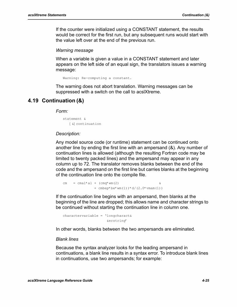
acslXtreme Statements Continuation (&)
If the counter were initialized using a CONSTANT statement, the results would be correct for the first run, but any subsequent runs would start with the value left over at the end of the previous run.
Warning message
When a variable is given a value in a CONSTANT statement and later appears on the left side of an equal sign, the translators issues a warning message:
Warning: Re-computing a constant.
The warning does not abort translation. Warning messages can be suppressed with a switch on the call to acslXtreme.
4.19 Continuation (&)
Form:statement &
[&]continuation
Description:
Any model source code (or runtime) statement can be continued onto another line by ending the first line with an ampersand (&). Any number of continuation lines is allowed (although the resulting Fortran code may be limited to twenty packed lines) and the ampersand may appear in any column up to 72. The translator removes blanks between the end of the code and the ampersand on the first line but carries blanks at the beginning of the continuation line onto the compile file.
cm = cmal*al + (cmq*wm(2) & + cmbep*be*wm(1))*d/(2.0*vmam(1))
If the continuation line begins with an ampersand, then blanks at the beginning of the line are dropped; this allows name and character strings to be continued without starting the continuation line in column one.
charactervariable = ‘longcharact& &erstring’
In other words, blanks between the two ampersands are eliminated.
Blank lines
Because the syntax analyzer looks for the leading ampersand in continuations, a blank line results in a syntax error. To introduce blank lines in continuations, use two ampersands; for example:
acslXtreme Language Reference Guide 4-25
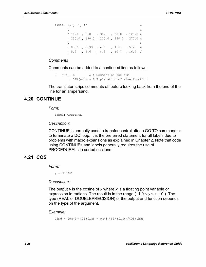
acslXtreme Statements CONTINUE
TABLE xyz, 1, 10 & & &
/-10.0 , 0.0 , 30.0 , 60.0 , 120.0 &
, 150.0 , 180.0 , 210.0 , 240.0 , 270.0 & & &
, 8.33 , 8.33 , 4.0 , 1.6 , 5.2 &
, 5.2 , 6.6 , 8.3 , 10.7 , 16.7 /
Comments
Comments can be added to a continued line as follows:x = a + b & ! Comment on the sum
+ SIN(a/b)*m ! Explanation of sine function
The translator strips comments off before looking back from the end of the line for an ampersand.
4.20 CONTINUE
Form:label: CONTINUE
Description:
CONTINUE is normally used to transfer control after a GO TO command or to terminate a DO loop. It is the preferred statement for all labels due to problems with macro expansions as explained in Chapter 2. Note that code using CONTINUEs and labels generally requires the use of PROCEDURALs in sorted sections.
4.21 COS
Form:y = COS(x)
Description:
The output y is the cosine of x where x is a floating point variable or expression in radians. The result is in the range (−1.0 ≤ y ≤ + 1.0 ). The type (REAL or DOUBLEPRECISION) of the output and function depends on the type of the argument.
Example:simd = (wm(2)*COS(fim) - wm(3)*SIN(fim))/COS(thm)
4-26 acslXtreme Language Reference Guide
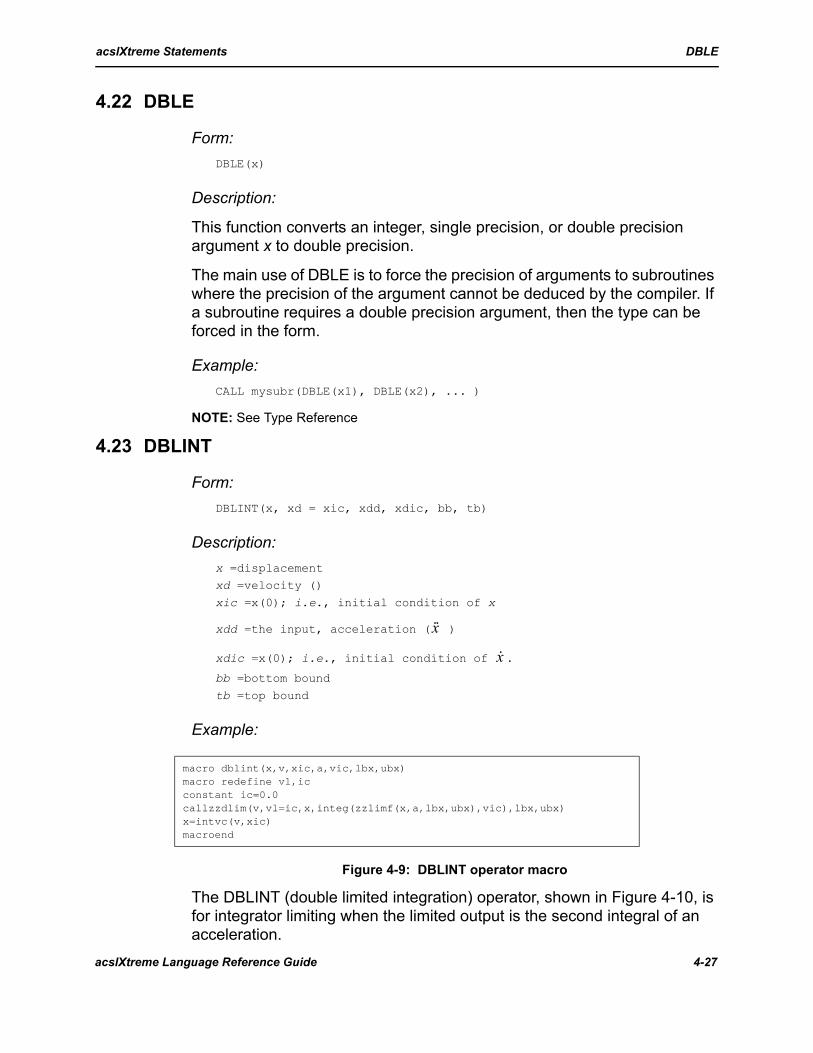
acslXtreme Statements DBLE
4.22 DBLE
Form:DBLE(x)
Description:
This function converts an integer, single precision, or double precision argument x to double precision.
The main use of DBLE is to force the precision of arguments to subroutines where the precision of the argument cannot be deduced by the compiler. If a subroutine requires a double precision argument, then the type can be forced in the form.
Example:CALL mysubr(DBLE(x1), DBLE(x2), ... )
NOTE: See Type Reference
4.23 DBLINT
Form:DBLINT(x, xd = xic, xdd, xdic, bb, tb)
Description:x =displacementxd =velocity ()
xic =x(0); i.e., initial condition of x
xdd =the input, acceleration ( )
xdic =x(0); i.e., initial condition of .
bb =bottom bound
tb =top bound
Example:
Figure 4-9: DBLINT operator macro
The DBLINT (double limited integration) operator, shown in Figure 4-10, is for integrator limiting when the limited output is the second integral of an acceleration.
macro dblint(x,v,xic,a,vic,lbx,ubx)macro redefine vl,icconstant ic=0.0callzzdlim(v,vl=ic,x,integ(zzlimf(x,a,lbx,ubx),vic),lbx,ubx)x=intvc(v,xic)macroend
x··
x·
acslXtreme Language Reference Guide 4-27

acslXtreme Statements DBLINT
Figure 4-10: Alternate implementation for DBILINT
Mass-spring damper system
This type of limiting can best be explained in terms of the mass-spring-damper system described by:
such that:
where physical stops constrain the mass to move only between xbb (bottom bound) and xtb (top bound); i.e.,
xbb < x < xtb
When the displacement (x) of the mass reaches its limit, the mass must stop, implying that the velocity ( ) is zero. The mass must remain stopped until the force acting on it (f (t) - cx) changes sign.
Alternate implementation
An alternate way of performing this operation is to wrap a stiff spring around the loop when the wall is approached; this corresponds to what happens physically since the wall always has a finite spring constant. Figure 4-10 is a block diagram of such a system where Ks is spring stiffness, Kw wall stiffness, and Kd the damping constant. The problem with this representation is in the behavior of the digital integration routine in the vicinity of the wall when the wall stiffness is extremely high. A more accurate but more complex approach is to use the SCHEDULE operator to
mx·· bx· cx+ + f t( )=
x· 0( ) xdicx 0( ) xic
==
x·
4-28 acslXtreme Language Reference Guide

acslXtreme Statements DEAD
find times of both wall impact and wall leaving (when the force changes sign or crosses zero).
NOTE: This operator (as all memory operators) can be used only in DERIVATIVE sections and should not be put in a PROCEDURAL block.
4.24 DEAD
Form:y = DEAD(bb, tb, x)
Description:
The DEAD operator implements a dead zone in output y when x lies between a specified bottom bound bb and top bound tb. The results can be represented as follows:
y = x - bb ; x < bby = 0.0 ;bb < x < tby = x - tb ;x > tb
Example:
The dead zone operator could be used as follows:v2 = v1 + k*DEAD(vmn, vmx, v3)
4.25 DELAY
Form:y = DELAY(x, ic, tdl, nmx, delmin)
DELAY(y = x, ic, tdl, nmx, delmin)
Description:
x = the input (an arithmetic expression of arbitrary complexity).
ic = the initial value of the output until the independent variable has advanced by the delay, tdl. This argument must be a variable name (rather than a literal constant) for the runtime command REINIT to work. REINIT needs a name into which to store the current DELAY output as the initial condition for subsequent runs.
tdl = the delay time between input and output (any expression with a value ≥ 0.0).
nmx = a literal integer giving the maximum number of saved data points needed to represent the delay. The integration step size may vary but the sum of nmx integration steps must always be greater than the current time delay.
acslXtreme Language Reference Guide 4-29
acslXtreme Statements DELAY
NOTE: This integer must be a literal integer or a parameter name with an integer value. For example:
co = DELAY(ci, cic, cdl, 1000, cmn)
Using a PARAMETER variable:INTEGER cmx
PARAMETER(cmx=1000)
co = DELAY(ci, cic, cdl, cmx, cmn)
This integer nmx allocates space in a circular buffer to hold the history data of previous sample times and previous input values. If delmin is defined, then nmx should be somewhat larger than the maximum delay times expected (tdl) divided by this delmin (or by the integration step if it is larger).
delmin= minimum interval between saving of data points in delay buffer. This argument may be omitted, in which case a default of zero is used. Typically delmin can be a tenth or a hundredth of the expected delay time and still represent dynamics adequately.
The DELAY operator delays a variable in time to model transport effects such as passage through a pipe. It should not be used lightly since it may require considerable storage unless delmin is specified.
Implementation
The DELAY operator is implemented by allocating a dummy array, 2*nmx words long, and prefilling it with the value of ic, extending over all past history. Each entry in the table is associated with a time, and at each new integration step (or delmin, whichever is larger) a new value is inserted into the array, treating it as a circular list. To compute the output value, tdl (the current time delay) is subtracted from the independent variable value and the table is searched for time values that bracket this required previous time. A linear interpolation is performed between the corresponding input values. If not enough data points are present, an error is reported and the run terminates.
Varying time delay
When tdl changes dynamically, this operator approximates the pipeline with a varying flow rate.
Direct feedback not allowed
The operator provides an algebraic path from input to output, so direct feedback (without an integrator) is illegal; the following for example is not allowed:
y = DELAY((n - y)/k, yic, tdl, 1000, 0.1)
4-30 acslXtreme Language Reference Guide

acslXtreme Statements DELSC
If direct feedback is really necessary, the output of the DELAY can be filtered through a real pole to break the loop. This is a good idea anyway since it eliminates jumps in the slope of the DELAY output produced by the straight line interpolation. For example:
y = REALPL(tfilt, DELAY((in - y)/k, yic, tdl, 1000, 0.1))
In this situation, TFILT is chosen to be small relative to the delay time (tdl).
4.26 DELSC
Form:state = DELSC(xn, ic)
DELSC(state = xn, ic)
Description:
state = a simple variable (DELVC handles vectors)
xn = an arithmetic expression of arbitrary complexity; i.e., may contain further DELSC statements or other functions or macros.
ic = a simple non-subscripted variable, a real constant, or a general expression enclosed in parentheses.
DELSC produces a one-step delay between the calculation of the xn value and its assignment to the state so that it shows up in the variable at the beginning of the next step.
DELSC may be embedded in any legal expression as a function that has a single output: the value of the state. When the delay statement is alone, then the state name can be identified; embedding it in an expression means that an acslXtreme-generated variable (i.e., in the form Znnnnn) is used for the state name.
NOTE: The DELSC statement can be placed only in a DISCRETE section, not a DERIVATIVE section.
With initial conditions
Since DISCRETE sections are not in general sorted, if an expression is used for the initial condition, then the DELSC expression must be placed before any reference to the state and after the calculation of the next value, so that this form is normally to be avoided. The implementation of the expression form involves the following expression:
if(zzicfl) state = ic
so it is only after the expression is seen that the states has a value the first time.
acslXtreme Language Reference Guide 4-31
acslXtreme Statements DELVC
In the more general case, the initial condition variable is equivalenced into the initial condition table and the values for all the states are moved at once before any DERIVATIVE or DISCRETE section code is executed at all.
Placement
In unsorted DISCRETE blocks, DELSC must be placed after the calculation of its inputs.
See the description of the INTEG statement for a general description of the way the acslXtreme system build tables of states, derivatives, and initial conditions. DELSC places the state in the state table, the next state in the derivative table, and the initial condition value in the initial condition table. The integration algorithm knows to update the delay state variables by:
xn+1 = xn
whereas the continuous states are updated by:xn+1 = xn + h*xd(effective)n
Examples of the use of the DELSC statement include:y = DELSC(5.0*(x(2) + c), yz)
x = 4.0*DELSC(4*y, 0)
z = DELSC(znext, zic)
4.27 DELVC
Form:x = DELVC(xn, xic)
DELVC(x = xn, xic)
Description:
Where X, XN, and XIC are arrays of the same size and correspond to state, derivative, and initial conditions, respectively.
The restrictions on the DELSC operator with regard to arrays can be avoided by using this vector integrator operator. The restrictions on the DELVC operator are identical to those on the INTVC operator with the additional one that the DELVC statements can appear only inside DISCRETE blocks.
In unsorted DISCRETE blocks, DELVC must be placed after the calculation of its inputs.
4-32 acslXtreme Language Reference Guide

acslXtreme Statements DERIVATIVE
Example:DIMENSION x(1), xic(10), m(5,5), mn(5,5), mic(5,5)
y = DELVC(yn, yic) ! scalar delayx = DELVC(xn, xic) ! vector delay
m = DELVC(mn, mic) ! matrix delay
4.28 DERIVATIVE
Form:DERIVATIVE [name]
...
END
Description:
The DERIVATIVE keyword identifies the beginning of a block of code performed at the request of the integration routine to evaluate the state variable derivatives. The DERIVATIVE statement must be paired with a matching END statement.
Implementation
The integration routine is called from the DYNAMIC section and asked to advance the state over the next communication interval using the code embedded in the DERIVATIVE blocks to evaluate the state variable derivatives; i.e., the integration algorithm calls the DERIVATIVE section. The actual number of evaluations depends on the integration algorithm employed.
Transfers illegal
All the statements in the DERIVATIVE section are translated into a separate subroutine, so it is illegal to transfer control by GO TO’s from DERIVATIVE sections to other sections (INITIAL, DYNAMIC, DISCRETE, or TERMINAL) or vice versa.
Barriers at CINT, DISCRETE, or SCHEDULE
The only break in the regular progression is at a communication interval or at an equivalent barrier represented by a DISCRETE section or a SCHEDULE event. The times for all DISCRETE, SCHEDULE, and communication actions are entered onto the event list where all actions are ordered in time; the next time on the event list is called the barrier time.
For the DERIVATIVE block, the current step size is checked against the current time (T) and the barrier time from the next event list. If integration with the current step size would exceed the barrier time, the actual step is
acslXtreme Language Reference Guide 4-33

acslXtreme Statements DERIVT
reduced so that the last step is made exactly up to the event. All states then line up in time for the event to take place.
CINT as integer multiple of step size
Integration step sizes and communication intervals are usually chosen to be integer multiples of each other. The acslXtreme system does not require this. For example, it is acceptable to choose a fixed step length for the continuous section of 4 msec, a sampling INTERVAL in the DISCRETE block of 11 msec, and a communication interval of 20 msec. The first few integration step sizes would then be (in msec):
4, 4, 3, 4, 4, 1, 2, 4, 4, 3, 4, 3, 4, ...
The first short step of 3 msec brings time up to 11 msec, the first barrier time, which is due to the DISCRETE section. Then two more normal steps are followed by a short step of 1 msec to bring time up to the communication time of 20 msec. The next barrier is the DISCRETE block at 22 msec causing a step size of 2 msec, and so on. Variable step algorithms look ahead to the next barrier to compute a constant step size which reaches the barrier without requiring a final short step.
4.29 DERIVTForm:
y = DERIVT(ic, x)
DERIVT(y = ic, x)
Description:ic = y(0)x = the input (an arithmetic expression)
The derivative function differentiates x and can be implemented if absolutely necessary.
NOTE: It is never necessary to invoke a derivative. The derivative can be expressed instead in terms of all the other states in the system.
Since the derivative operator is a first order approximation, it can lead to instability if it is used to represent any major loop. The only time this may be justified is for a minor term where a large amount of extra calculation may be needed to reform the problem in terms of the states.
PID example
As an example of how DERIVT can be avoided, consider the D term in a PID (proportional, integral, derivative) controller. There is a tendency to use
4-34 acslXtreme Language Reference Guide
acslXtreme Statements DIM
DERIVT for this term, but in hardware, it is always implemented by a differentiation over a first order lag; i.e.,
This formulation can be represented by a single line of acslXtreme code:y = (k*x - INTEG(y, ic))/t1
Nature never has a free differentiator; it is always combined with a lag to make it realizable.
Example
An example of a DERIVT statement could be:ald = DERIVT(alic, al)
4.30 DIM
Form:y = DIM(x1, x2)
Description:
The output y is the positive difference between x1 and x2 where x1 and x2 can be variables or expressions. DIM takes its type and types its output based on the type of the arguments. The result can be represented as follows:
y = x1 - x2 ;x1 > x2
y = 0.0 ; otherwise
The following logic is often used:
Jabobian The use of DERIVT invalidates the Jacobian calculation from the ANALYZE command, including all the derived data (zeros, root locus, and frequency response plots). This is another good reason not to use DERIVT.
Sorting The DERIVT operator (as all memory operators) should be used only in sorted sections and should not be put in a PROCEDURAL block.
Initial Condition Use a variable name rather than a literal constant for the initial condition so that REINIT has a place to store it; otherwise REINIT tries to overwrite the global zero with the one in the common block.
yx--
KsT1s 1+-----------------=
acslXtreme Language Reference Guide 4-35
acslXtreme Statements DIMENSION
PROCEDURAL(x = y,z)x = y - z
IF(x .LT. 0.0) x = 0.0
ENDa = SQRT(x)
One line using DIM can solve the same problem:a = SQRT(DIM(y, z))
DIM is useful for representing cable spring stiffness. Negative extension cancels zero force with a cable.
4.31 DIMENSION
Form:DIMENSION v1(a...), v2(a...), ..., vn(a...)
Description:
The variable names vi may have up to six integer constant subscripts separated by commas; e.g., SPACE(5,5,5,5,5,5). The subscripts may be symbolic if the symbols are declared INTEGER and defined in a PARAMETER statement. This operator allocates space for up to six dimensions to be associated with a variable name. The statement can appear anywhere in the program, but it must appear before any invocation of a macro that uses dimension information.
Type declaration
Arrays can also be dimensioned using the REAL, DOUBLEPRECISION, or INTEGER statements. DIMENSION is preferred for floating point variables unless the type of precision needs to be forced. Using DIMENSION allows the type to adjust depending on the global option (single or double precision) selected.
NOTE: Names of certain acslXtreme macros should not be used as arrays. acslXtreme cannot check that the name defined as an array is also a macro because the TABLE statement defines an array to hold data and a macro of the same name for table lookup. The names of the following acslXtreme operators should not be used for arrays (as scalars is not a problem):
4-36 acslXtreme Language Reference Guide

acslXtreme Statements DISCRETE
Array order
Elements of arrays are written and accessed by column, then row; i.e., (a(i,j) where i = row, j = column). For example, the elements of b(2,5) can be shown:
11 12 13 14 15
21 22 23 24 25
Extracted as a single-demensioned vector, the order is:11 21 12 22 13 23 14 24 15 25
Examples
An example of a DIMENSION statement is:DIMENSION rm(3), em(3,3), hold(2,n), x(3,4,2,4,3,5)
4.32 DISCRETE
Form:DISCRETE [name]
...
END
Description:
The keyword DISCRETE introduces a section to be executed by either an INTERVAL statement or the SCHEDULE operator. The section is concluded by a matching END statement.
DISCRETE sections are intended primarily for modeling digital sampled data controllers where the communication to and from the continuous world occurs at fixed times known in advance. Another common application is changing state or other variables when a state event occurs (in which case
BCKLSH HISTORY LINES REALPL TRANZCMPXPL IMPL MODINT RESET UNIFDBLINT IMPLC OU RSHM UNIFIDELAY IMPVC OUTPUT RSHMI WDACDELAYP INTEG PREPAR RTDEVIC WDACFDERIVT INTVC PTR RTP WDIGDELVC LEDLAG RADC SCALE WDZGIDELSC LIMINT RADCI SMOOTH WSHMGAUSI LIMIT RDIG TERMT WSHMIGAUSS LINEAR RDIGI TRAN ZOH
acslXtreme Language Reference Guide 4-37
acslXtreme Statements DO
execution of the DISCRETE section is handled by a SCHEDULE statement).
Sorting
The translator does not automatically sort the code. Use the SORT keyword to have code within a DISCRETE section sorted. Code is never sorted across sections, nor are the sections themselves sorted.
Explicit structure level
DISCRETE sections are at the same level as any DERIVATIVE sections. If a DYNAMIC section is used, DISCRETE sections are placed inside it. (See Chapter 3 for further information on explicit program structure.)
Executed at discrete event
DISCRETE sections are executed at a discrete event or time point. The time of the execution is controlled by the keyword INTERVAL or by a SCHEDULE statement. Like the DERIVATIVE section, each DISCRETE section has a time associated with it that is entered into an event list. This time becomes a barrier for DERIVATIVE sections, ensuring that the integration routine takes a final step (which may be short) up to the barrier time before the code in the DISCRETE section is executed. If execution is controlled by an INTERVAL statement, the section is re-entered on the event list with a time of execution equal to the current time plus the current value of the INTERVAL variable.
4.33 DO
Form:DO n i = m1, m2[, m3]
...
n:CONTINUE
Description:
n = a label (numeric or symbolic) of the terminal statement of the loop.
i = a simple integer variable called the index variable. With each repetition, its value is altered by the increment parameter m3. This variable may not be changed within the loop.
m1 = initial parameter, the value of i during the first loop.
m2 = terminal parameter. When the value of i surpasses the value of m2, DO execution is terminated and control goes to the statement immediately following the terminal statement.
4-38 acslXtreme Language Reference Guide

acslXtreme Statements DOUBLE PRECISION
m3 = increment parameter, the amount i is increased with each repetition. The default value of m3 is 1.
The m1, m2, and m3 may be integer constants, variables, or expressions of arbitrary complexity; if variables, they must be declared explicitly to be INTEGER variables. A DO statement makes it possible to repeat a group of statements a designated number of times using an integer variable whose value is progressively altered with each repetition. The initial value, final value, and rate of increase of this integer variable are defined by the set of indexing parameters included in the DO statement. The range of the repetition extends from the DO statement to the terminal statement, which must follow the DO statement, and this whole sequence is called the DO loop.
PROCEDURAL in sorted sections
This is the standard DO statement. Using a PROCEDURAL is not necessary within INITIAL, DYNAMIC, DISCRETE, or TERMINAL sections.
Error checking
For more information on the structure of the DO statements, refer to the specific language reference manual. The acslXtreme translator checks the syntax of the DO statement but does not validate the correct nesting of loops or terminal statements. Errors of structure are indicated by the language compiler.
4.34 DOUBLE PRECISIONSee TYPE.
4.35 DYNAMIC
Form:DYNAMIC
...END
Description:
The DYNAMIC keyword identifies the beginning of a section of code that is performed every CINTERVAL communication interval throughout the run. It must be accompanied by a matching END statement.
The DYNAMIC section is the place to put output-related calculations so they can be performed at the usually slower data recording rate rather than at each derivative evaluation. Examples of calculations generally performed in this section are unit conversions (such as radians to degrees), which do not affect DERIVATIVE calculations. Most calculations
acslXtreme Language Reference Guide 4-39

acslXtreme Statements END
that affect code in the DERIVATIVE section should be in a separate DISCRETE section so model behavior is independent of the data recording action; the DYNAMIC section is not intended for computing variables to be input to DERIVATIVE or DISCRETE sections.
The time to the next communication interval can be calculated in the model, based on some simulation phase or configuration, thus obtaining variable data recording rates (see CINTERVAL for an example).
Code in the DYNAMIC block is not sorted automatically. Use the SORT keyword to have it sorted.
4.36 END
Form:END
Description:
An END statement denotes the end of a block (e.g., a PROCEDURAL block) or section (DYNAMIC, DERIVATIVE, etc.). Chapter 3 shows the use of ENDs in structuring an explicit program.
One of the most common errors in programming a model is not getting the right number of ENDs to balance the program sections. The following error messages are issued when the count is incorrect.
...Not enough ends
...Too many ends
The END statement acts like a right parenthesis in an arithmetic expression, except that it terminates blocks of statements; an incorrect count corresponds to unbalanced parentheses.
4.37 ERRTAG
Form:ERRTAG name
Description:
Where name is a simple unsubscripted variable. ERRTAG defines the system variable name that is used to indicate an attempt to reduce the step size below the minimum, MINT. This statement changes the name of the variable to a name of your choice. The value of this name is set TRUE to indicate an attempt by a variable step size integration algorithm to reduce the integration step size to satisfy the error bounds. The type of name is automatically set to LOGICAL and the value is preset to FALSE. The variable step integration routine calls the derivative subroutine once with
4-40 acslXtreme Language Reference Guide

acslXtreme Statements EXP
the name given under ERRTAG set to TRUE if it needs to reduce the step size below the specified minimum MINT. If it is still TRUE on return, the termination flag for that run is set. Control should then revert to the TERMINAL section (if any) and the executive, and the next runtime command is read. If provision is made to handle this case and reset the flag, then care must be taken that a very small step size does not result in excessive computer time being used.
4.38 EXP
Form:y = EXP(x)
Description:
The output y is the exponential of the floating point argument x, where x is limited in size such that the maximum machine word size should not be exceeded by the exponential.
Example:
The expression is represented mathematically:
y = ex
4.39 FCNSW
Form:y = FCNSW(p, x1, x2, x3)
Description:
The output y of the function switch operator is determined by the input function p as follows:
y = x1 p < 0.0y = x2 p = 0.0y = x3 p > 0.0
Note that zero almost never exists in the span of real numbers unless some other action forces it there.
Example: v = FCNSW(ain, vneg, vzer, vpos)
acslXtreme Language Reference Guide 4-41

acslXtreme Statements GAUSI, UNIFI
4.40 GAUSI, UNIFI
Form:GAUSI(k)
UNIFI(k)
Description:
The output of these functions is the seed for the random number generator. Input k is an integer constant or expression and should be a large, positive odd number for a maximal length sequence. The macro for and GAUSI operator macros is shown in Figure 4-11.
Figure 4-11: GAUSS and GAUSI operator macros
Only one of the initialization routines should be used since they both set the same seed variable; either may be used with any other routine as they perform exactly the same function.
The random number generators are provided with a default seed initialization, so these initialization routines are required only when you wish to override the default. The default seed number is 55555555.
The GAUSI or UNIFI operator should be invoked only in the INITIAL section of an explicit program, or provision must be made to skip over it except at the beginning of each run in an implicit program. If the operator is executed repeatedly, the random numbers do not change.
The seed need not be specified for each invocation of the random number generators since subsets of random sequences are also uncorrelated random sequences.
MACRO gauss(y,ave,sig)
MACRO REDEFINE grv
REAL grv
CALL zzgrv(grv=zzseed)
y = ave + grv*(sig)
MACROEND
MACRO gausi(seed)
PROCEDURAL(=seed)
zzseed=seed
END
MACROEND
4-42 acslXtreme Language Reference Guide

acslXtreme Statements GAUSS
4.41 GAUSS
Form:y = GAUSS(m, s)
GAUSS(y = m, s)
Description:
Where m is the mean and s is the standard deviation. The output y is a normally distributed random variable. Figure 4-11 gives a listing of the operator macro.
Seed
The seed for a random sequence can be reset by UNIFI or GAUSI. If not set, a different random sequence is in effect for each run.
NOTE: GAUSS is not intended for use in a DERIVATIVE section because the power density (or, what is usually more important, the low frequency power) depends on the integration step size. Instead, use the OU operator.
Example:vmic = GAUSS(0.0, vmsg)
4.42 GO TO
Form:GO TO label
GO TO (n1, n2, ..., nm), i
Description:
Where ni are statement labels that correspond to a possible label and i is a simple integer variable that has been given a value between 1 and m. GO TO statements transfer control to labeled statements whose references are fixed or which are assigned during execution of the program.
Transfers between sections
The statement labels used in the GO TO statements must be associated with executable statements in the same program unit as the GO TO statement. In explicit programs, the INITIAL, DYNAMIC, and TERMINAL sections exist in a single program unit. However, control cannot be transferred into the DYNAMIC region. The reason for this is that the integration routines must be initialized at the start of the run; this initialization operation is done on leaving the INITIAL section and entering the DYNAMIC section. Control can be transferred from the DYNAMIC
acslXtreme Language Reference Guide 4-43

acslXtreme Statements HARM
region to the INITIAL or TERMINAL section and between INITIAL and TERMINAL sections.
DERIVATIVE DISCRETE
The DERIVATIVE section is a separate program block and control cannot be transferred into or out of it. Control also cannot be transferred between DISCRETE and DYNAMIC, INITIAL, or TERMINAL sections because DISCRETE sections are in the same subroutine as the DERIVATIVE section.
Statement labels
A statement label may be either numeric or symbolic. Execution resumes at the statement with the referenced label. We recommend using a CONTINUE as the labeled statement to avoid possible problems with sorting.
Example:
Examples of valid GO TO statements include:GO TO loop
GO TO (100, 200, 300, 400, 500), ibin
A large number of GO TOs is considered harmful to the successful completion of any simulation project.
4.43 HARM
Form:y = HARM(tz, w, p)
The output y is a sinusoidal or harmonic drive function with the results:y = 0.0 T < tzy = sin (w ∗ (T − tz ) + p ) T ≥ tz
Descrption:tz = delay (sec)
w = frequency (rad/sec)p = phase shift (rad)
Note that if p is nonzero, a discontinuity is involved.
Example:drive = HARM(tdrive, w1, phased)
4-44 acslXtreme Language Reference Guide
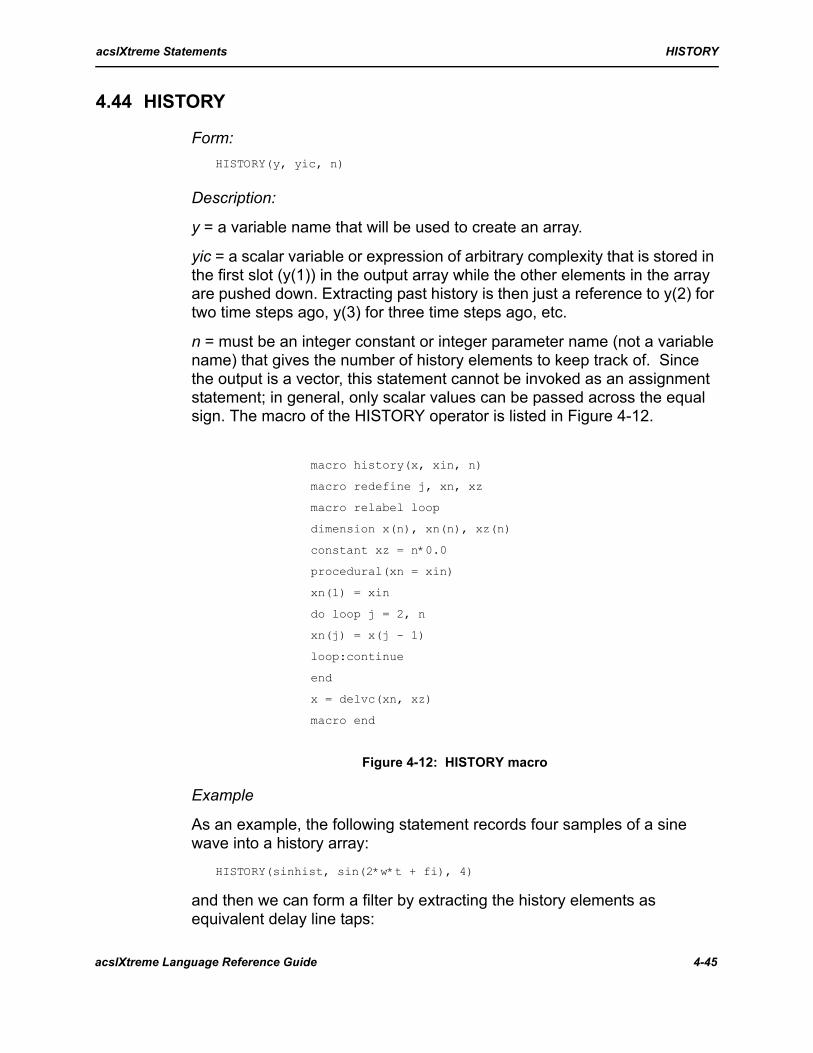
acslXtreme Statements HISTORY
4.44 HISTORY
Form:HISTORY(y, yic, n)
Description:
y = a variable name that will be used to create an array.
yic = a scalar variable or expression of arbitrary complexity that is stored in the first slot (y(1)) in the output array while the other elements in the array are pushed down. Extracting past history is then just a reference to y(2) for two time steps ago, y(3) for three time steps ago, etc.
n = must be an integer constant or integer parameter name (not a variable name) that gives the number of history elements to keep track of. Since the output is a vector, this statement cannot be invoked as an assignment statement; in general, only scalar values can be passed across the equal sign. The macro of the HISTORY operator is listed in Figure 4-12.
Figure 4-12: HISTORY macro
Example
As an example, the following statement records four samples of a sine wave into a history array:
HISTORY(sinhist, sin(2*w*t + fi), 4)
and then we can form a filter by extracting the history elements as equivalent delay line taps:
macro history(x, xin, n)
macro redefine j, xn, xz
macro relabel loop
dimension x(n), xn(n), xz(n)
constant xz = n*0.0
procedural(xn = xin)
xn(1) = xin
do loop j = 2, n
xn(j) = x(j - 1)
loop:continue
end
x = delvc(xn, xz)
macro end
acslXtreme Language Reference Guide 4-45
acslXtreme Statements IF, IF-THEN-ELSE
filt = b0*sinhist(1) + b1*sinhist(2) + b4*sinhist(4)
Placement
HISTORY can appear only in DISCRETE sections since it makes use of the DELVC operator to delay the history elements. In unsorted DISCRETE sections, HISTORY should be placed after the calculation of all its input variables. The elements of the array are initialized to zero the first time.
4.45 IF, IF-THEN-ELSE
Form:IF(lexpr) statement
IF(lexpr) THENblock1
ELSE IF(lexpr1) THEN
block2ELSE
block3
END IF
Description:
IF statements are used to transfer control or perform calculations conditionally. At the time of execution, an expression in the IF statement is evaluated and the result determines whether the rest of the statement is executed.
The logical expression lexpr is a logical or relational expression, one that produces a single value (either TRUE or FALSE).
Logical IF
Description:
In the logical IF form, statement is any executable statement. Only a single statement can be included in the logical IF statement.
Examples:IF(a .LT. 5.0) a = a + 0.1
PROCEDURAL(x = )
IF(x .GT. xmax) GO TO finishx = k*xprev
xprev = x
finish: CONTINUE
END
Logical IF statements that transfer control in sections that are sorted by acslXtreme (DERIVATIVE sections or implicit programs) must be enclosed
4-46 acslXtreme Language Reference Guide

acslXtreme Statements IF, IF-THEN-ELSE
in PROCEDURAL blocks, as in the second example, in order to maintain statement order. This example however would be better handled with a block IF construct.
Block IF
Description:
Block IF statements conditionally execute blocks (groups) of statements, a sequence of zero or more complete CSL statements including other IF-THEN-ELSE blocks. Such a sequence is called a statement block.
Examples:IF(ABS(force) .GT. breakout) THEN
vdot = netforce/mass
ELSEvdot = 0.0
END IF
IF(a .GT. b) THEN
d = b
f = a - bELSE IF(a .GT. b/2) THEN
d = b/2
f = a - b/2END IF
Initializing variables
Note that the same output variables should always be defined in all branches of the logic. If they are not, the last value placed in the variable is left around and used in subsequent integration steps. For example, in the following code, either VDOT or YDOT is not initialized:
IF(a .GE. b) THEN
vdot = f(a)
ELSE ydot = f(b)
END IF
Assuming A starts off less than B, then VDOT is not given a value but YDOT is. When A becomes greater than or equal to B, then VDOT is given a value but YDOT continues to hold its last value. This is not necessarily wrong, just an issue to consider when coding logic.
acslXtreme Language Reference Guide 4-47

acslXtreme Statements IMPLC
Statements on same line
The IF-THEN statement takes no additional statements on the same line unless the separator (a semi-colon) is used, turning it into a separate statement; e.g.,
IF(lexpr) THEN ; I = 1 ; ENDIF
Memory operators
Memory operators such as INTEG, REALPL, TRAN, etc. should not be used inside statement blocks. It’s possible to step over an integration statement with logic, but that doesn’t stop the integration from taking place; it just means that the derivative is not being calculated. This results in the last calculated value being used. If you don’t want a state to be integrated, make the derivative zero.
PROCEDURAL
PROCEDURAL blocks are used to hide logical code from the translation sorting process, but IF blocks are moved as one and don’t require the PROCEDURAL. The sorting algorithm looks at all the outputs of the block (those variables on the left side of an equal sign) and all the inputs (those variables on the right side of an equal sign) and positions the block according to the normal sorting rules. Thus the block is placed after the calculation of all the input variables and before the use of any of the output variables.
4.46 IMPLC
Form:z = IMPLC(r, zic)
Description:
z = a simple algebraic variable (IMPVC handles vectors)
r = residual, an arithmetic expression of arbitrary conplexity (i.e., may contain functions, macros, or other integration statements)
zic = a simple unsubscripted variable, a floating point constant, or a general expression enclosed in parentheses. If it is a simple variable (preferred), then this variable name must not be used as another initial condition, state, derivative, or system variable name.
Implicit integration
In implicit integration, algebraic constraints are defined by an expression that evaluates to a residual; this residual is then kept at or close to zero.
4-48 acslXtreme Language Reference Guide
acslXtreme Statements IMPLC
One use of this feature is in solving for pressure or voltages at junctions, where the junction has flows or currents that sum to zero (Kirchoff’s Law). Specifying the unknown quantity (pressure or voltage) as dependent on the residual of the sum of the flows allows it to be adjusted until the sum is really zero.
Examples
The example Tank with Boiling Benzene in Appendix A illustrates a PI controller with the implicit operators. The aircraft example ACRFTS also uses IMPLC.
Must be in DERIVATIVE
The implicit operators must be in DERIVATIVE sections, and they cannot be skipped over in logical structures such as PROCEDURAL or IF-THEN-ELSE blocks.
Residual
The residual expression must be related to the algebraic variable by a path such that the partial derivative of all the residuals, taken as a vector with respect to all the algebraic variables again taken as a vector, is a non-singular matrix.
The state and algebraic variables can be seen more clearly in the following:Y = F(Y, Z )
0 = G(Y, Z )
Here the Y’s are the state variables and the Z’s are the algebraic variables. This is now expressed for scalars as:
y = INTEG(F(Y, Z), yic)z = IMPLC(G(Y, Z), zic)
or, for vectors:y = INTVC(f, yic)
z = IMPVC(g, zic)
where now F and G are vectors that have been filled with derivatives and residuals respectively in a separate operation. Of course scalar and vector variables can be used and mixed freely. The acslXtreme translator builds a complete vector of states and a complete vector of residuals for all the component parts.
acslXtreme Language Reference Guide 4-49

acslXtreme Statements IMPLC
Since we must be able to solve the residual relationships for Z, this means that the partial of G with respect to Z must be non-singular; i.e.,
Derivative
It sometimes is not possible to extract the derivative explicitly from the left-hand side of an equation, so that the model equations are expressed as:
To handle this, case we have overloaded the IMPLC and IMPVC syntax by defining a second variable on the left. For scalars, the above equation would be written:
y, yd = IMPLC(F(y,yd,t), yic)
In actual implementation, this is transformed into an integration statement and an algebraic constraint as follows:
y = INTEG(yd, yic)
yd = IMPLC(F(y,yd,t), 0.0)
DAE Implementation
The acslXtreme translator builds up vectors for states, derivatives, and initial conditions using the INTEG and INTVC operators. At this level, we have added to these vectors the algebraic variables (to the state vector), residuals (to the derivative vector), and initial guesses for the algebraic variables (to the initial condition vector). These now look like the following:
Figure 4-13: Layout of state vectors
states derivatives ICs
s1 d1 ic1
s2 d2 ic2
s3 d3 ic3
... ... ...
a1 r1 ig1
a2 r2 ig2
a3 r3 ig3
∂G Y Z,( )∂Z
---------------------- 0≠
F9 Y Y· T, ,( ) 0=
4-50 acslXtreme Language Reference Guide

acslXtreme Statements IMPVC
or, linearizing:
Since R is nominally zero, the second line leads to:
GYY = -GZZ
and:
This matrix is the one used in the Gear stiff algorithm since every time the derivatives are evaluated the Z variables are simultaneously adjusted to force the residuals to zero.
The nonlinear equation solver to find the Z variables is similar to the one used by the runtime ANALYZE command. It essentially computes a Newton-Raphson step:
and a steepest descent step:
Then it takes a linear combination of these two calculations depending on how successful the iteration is or has been. Since changes are usually small from one iteration step to the next, this iteration usually converges in one or two evaluations using the Newton-Raphson step. The usual problem is finding the algebraic (Z) variable at the very beginning when the initial guesses may be far from the true solution.
An example using the implicit scalar operator is:residtl = htotal - hl(t1) - hv(t1)
tl = IMPLC(residtl, tlic)
4.47 IMPVC
Form:z = IMPVC(r, zic)
Y·R
F Y Z,( )G Y Z,( )
=
Y·R
FyFzGYGZ
YZ
=
Y· Fy FZGZ1– GY–( )Y=
δNR GZ1– R=
δSD GZTR=
acslXtreme Language Reference Guide 4-51

acslXtreme Statements INCLUDE
Description:
Where Z, R, and ZIC are arrays of the same size and correspond to algebraic variable, residual, and initial condition, respectively. The mechanization of this operator is explained under IMPLC above.
Restrictions apply to the IMPVC operator that are similar to those for vector integration, INTVC; i.e.:
1. IMPVC cannot be used in an expression.
2. The residual array cannot appear any where else as a state, algebraic variable, or initial condition.
3. The initial condition must be a variable name, it cannot be a literal constant or an expression.
4. The array size may be one, or, equivalently, a simple undimensioned variable can be used instead. In this case, the residual name is equivalenced directly into the array of residuals and no extra assignment statement is generated.
Example:PROCEDURAL(rv = a,b)
rv(1) = a + b
rv(2) = c - bEND
x = IMPVC(rv, xz)
4.48 INCLUDE
Form:INCLUDE ‘filename’
Description:
Where ‘filename’ is in single quotes and conforms to the local operating system syntax.
Example:
On a Unix system, statement could be in the form:INCLUDE ‘../mod1.inc’
and under VAX/VMS as follows:INCLUDE ‘[-]mod1.inc’
Environment variables
The syntax of the file name supports references to operating system environment variables through the use of a prepended dollar sign ($). For example, if HOME is an environment variable defined in the Unix or
4-52 acslXtreme Language Reference Guide

acslXtreme Statements INITIAL
Windows operating system, then the INCLUDE statement will find a file (xyz.inc) in the user’s home directory:
INCLUDE ‘$HOME/syz.inc’
Paths
The environment variable is explanded into the full path for the file, including adjustment for differences in forward or backward slashes for the machine operation system. If on a PC, forward slashes (/) are changed to back slashes (\), and if on a Unix system, the opposite applies, so a common source file can be used for running on both PC and Unix systems.
Procedure
The INCLUDE statement directs the acslXtreme translator to suspend reading statements from the current file and read the statements from the INCLUDE file. The INCLUDE file must comprise complete acslXtreme statements and must result in a valid program when combined with the surrounding code.
INITIAL, DYNAMIC, TERMINAL
INCLUDE files can contain separate INITIAL, DYNAMIC, and/or TERMINAL sections with their matching END statements. These blocks are added to the current sections being built as the acslXtreme translator works its way through the model definition file.
Example
An example of using INCLUDE files is to break a simulation into modules which are then brought into a skeleton; e.g.,
DERIVATIVE
INCLUDE ‘seeker.inc’INCLUDE ‘autopilot.inc’
INCLUDE ‘actuator.inc’
INCLUDE ‘airframe.inc’END ! of derivative
Nesting
INCLUDE files can themselves contain other INCLUDE statements.
4.49 INITIAL
Form:INITIAL
...
END
acslXtreme Language Reference Guide 4-53
acslXtreme Statements INT
Description:
The INITIAL keyword identifies the beginning of a section of code that is performed just once at the start of each run. The INITIAL statement must have a matching END statement. Refer to Chapter 3 for rules of explicitly structured programs.
Sorting
Code within the INITIAL section is not automatically sorted. Use the SORT keyword to have an INITIAL section sorted.
Multiple INITIAL sections
Any number of INITIAL sections may be used within a program, at any nesting level. This feature is particularly useful in conjunction with INCLUDE files and/or acslXtreme macros; i.e., modules can be developed in separate files with their own INITIAL sections, then brought into a DERIVATIVE section in a larger model by means of INCLUDE statements.
The translator collects all the INITIAL sections in the order encountered and adds them to the end of the INITIAL section to be executed. If the sections of code to be added need to be in a particular order (so that a variable is defined before being used, for example), the SORT keyword can be used.
NOTE: MACROs with INITIAL sections cannot be called from within PROCEDURAL sections. This is because at the moment the INITIAL keyword must be at a PROCEDURAL nesting level of zero.
4.50 INT
Form:n = INT(x)
Description:
The output n is the integerization of the argument x. The implementation is that n is the sign of x times the largest integer ≤ | x |. INT could be used as in the following example:
INTEGER ibin, ibin1
ibin = ibin1 + INT(xz + x*y)
Example:
INT or AINT can be used on the right side of an equal sign; y = INT(x)
4-54 acslXtreme Language Reference Guide
acslXtreme Statements INTEG
In this case, the value of x is integerized, but then the result is floated according to normal conversion rules. The type of the arguments to subroutines however cannot be inferred, so INT or AINT must be chosen to match the argument type. In the following, for example, the first argument is forced to be INTEGER and the second, REAL.
CALL mysubr(INT(x1), AINT(x2), ...)
Now the arguments won’t change type with a change in the acslXtreme translator mode.
4.51 INTEG
Form:state = INTEG(deriv, ic)
Description:
state = a simple variable. (INTVC handles integration of vectors.)
deriv = an arithmetic expression of arbitrary complexity; i.e., may contain further INTEG statements, functions, or macros.
ic = a simple non-subscripted variable, a real constant, or a general expression enclosed in parentheses. If it is a simple variable (preferred), then this variable name must not be used as another initial condition, state, derivative, or system variable name. If an expression is used, both the initial condition and the state are given dummy variable names; a consequence of this is that XERROR and MERROR do not recognize the state name.
INTEG may also be embedded in any legal expression as a function that has a single output, the value of the state. When the integration statement is alone, then the state name can be identified; embedding it in an expression means that an acslXtreme-generated variable (i.e., in the form Znnnnn) must be used for the state name.
Initial conditions as expressions
If an expression is specified for an initial condition, the expression is sorted in such a way that all components in the expression are evaluated before the state value is assigned in the first (initialization) evaluation of the derivatives. Equations using the state then follow. Problems may occur when using this form with the REINIT command at runtime. The expression is always evaluated and substituted for an initial condition established by the reinitialization operation.
acslXtreme Language Reference Guide 4-55

acslXtreme Statements INTEG
Implementation
All integration in an acslXtreme program is handled by a centralized integration routine. In performing integrations, the integration algorithms utilize two intervals: (1) the integration step size and (2) the communication interval. Since digital integration is basically a discrete process, the integration step is the fundamental interval over which the state variables are updated. No finer detail is accessible except by some interpolation method. All integration schemes for the set of first order differential equations in the form:
are transformed into:
where (0.0 ≤ α ≤ 1.0) and h is the integration step size. The problem is to find the effective derivative to use in updating the state vector. Note that with suitable conditions on continuity and differentiability, the mean value theorem guarantees that an α exists that produces an exact answer for the state trajectory; finding it is another matter, however. Different integration schemes approximate the derivative in different ways, usually by expanding the derivative function in a Taylor series about the current state. For an example of how this is implemented, see the explanation of the Runge-Kutta fixed-step fourth order algorithm in the section on ALGORITHM.
Examples
Examples of use of the INTEG statement include:y = INTEG(5.0*x(1) + c, yic)z = p*INTEG(zdot, 0.0) + bt
w = INTEG(wdot, (2.0*al*SIN(th)))
Z in the above is not a state since the INTEG function appears embedded in an expression.
Integrating vectors
The INTVC operator should be used for integrating vectors or multidimensional arrays.
Initial condition names
Names of initial conditions can be only names not used as states, other initial conditions, or system variables. The following statements are all illegal when used with above example statements, except that CINT can be used if the system default name for the communication interval has been changed with a CINTERVAL statement:
x· f x( )=
xn 1+ xn h∗f xn α+( )+=
4-56 acslXtreme Language Reference Guide
acslXtreme Statements INTEGER
yy = INTEG(yyd, yic) ! yic is IC for y defined abovezz = INTEG(z*4.0, w) ! w is a state defined above
zk = INTEG(kk, CINT) ! CINT is a system variable
4.52 INTEGERSee TYPE.
4.53 INTERVAL
Form:INTERVAL name = floating point number
Description:
where name is a simple unsubscripted variable name. The INTERVAL statement schedules repeated execution of a DISCRETE section and can be used only in a DISCRETE section. It is used to define both the name of the variable controlling the repetition period and its initial value.
No defaults
There is no default for the INTERVAL name or value. A DISCRETE section without an INTERVAL statement is not executed automatically. An alternative means of activating a DISCRETE section is with a SCHEDULE statement.
An example of an INTERVAL statement could be:DISCRETE dac INTERVAL dt = 0.1
...
END
In MINT array
The mechanization of the INTERVAL feature is to use the slot in the global MINTERVAL array corresponding to the DISCRETE section. The INTERVAL variable is equivalenced into this array. If no INTERVAL statement is placed within the DISCRETE block, a value of -1.0 is used as the default. This flags the DISCRETE section as not to be executed during the initialization phase.
Changing value
The INTERVAL value may be changed (anywhere in the program, or at runtime). It is the value which is current when the DISCRETE section has completed execution which determines the next execution time. Once the DISCRETE section is on the event list, changes in the INTERVAL value do not affect the next execution time.
acslXtreme Language Reference Guide 4-57
acslXtreme Statements INTVC
Strobe effect
When the INTERVAL for activating a DISCRETE section is a decimal fraction, it is possible for small errors in timing to result in a beating or strobe effect. The problem is that decimal fractions (0.1 for example) are never exact on a binary machine. In order to maintain accuracy, acslXtreme finds an integer multiplier of CINTERVAL such that the result is an integer (to machine accuracy). If CINT is 0.1, for example, the multiplier is 10. The communication interval times are obtained by accumulating integer ones and finding the end point by dividing by ten. A thousand 0.1s by this method is 100 exactly, while a thousand additions of 0.1 (not a power of two and so a rounded number) has significant error. Since CINT is adjusted and INTERVAL statements are not, a difference can develop. If this is an important consideration, double precision can help, or else the INTERVAL value can be biassed by setting it to, for example, 0.1000001 or 0.099999999 instead of 0.01.
4.54 INTVC
Form:x = INTVC(xd, xic)
Description:
where x, xd, and xic are arrays of the same size and correspond to state, derivative, and initial condition, respectively. The missile example in Appendix A uses INTVC.
Restrictions
The restrictions on the INTEG operator with regard to arrays can be avoided by using this vector integrator operator. The restrictions on the INTVC operator are as follows:
1. INTVC cannot be used in an expression.
2. The derivative array must not appear anywhere else as a state. If a state must be used as a derivative (velocity, for instance, which has been integrated from acceleration and is then the derivative of range), use the block transfer (XFERBR) subroutine to move it into another array before using INTVC.
3. The initial condition must be a variable name; it cannot be either a constant or an expression.
4. The array size may be one. A single undimensioned variable can also be used, in which case, the derivative name is used explicitly and no extra assignment statement is generated. INTVC is the preferred method for integrating scalars if the derivative is a scalar as well.
5. The derivative array cannot be preset with a CONSTANT statement since it is cleared automatically to a small number before the derivative evaluation
4-58 acslXtreme Language Reference Guide

acslXtreme Statements LEDLAG
routine is called the first time (at the end of the INITIAL section) after every START.
Examples
Following are examples using INTVC:DIMENSION x(10),xd(10),xic(10),m(5,5),md(5,5),mic(5,5)
y = INTVC(yd, yic) ! scalar integration
x = INTVC(xd, xic) ! vector integrationm = INTVC(md, mic) ! matrix integration
NOTE: A variable cannot be a derivative in one INTVC statement and a state in another. For example, if r, v, and a are range, velocity, and acceleration vectors:
DIMENSION r(3), ric(3), v(3), vic(3), a(3)
the following is illegal:v = INTVC(a, vic)
r = INTVC(v, ric)
since these statements ask for v to be considered as both a state and a derivative at the same time. Using the XFERBR (transfer block) subroutine and defining an RD (R dot) array, the sequence becomes:
DIMENSION r(3), rd(3), ric(3), v(3), vic(3), a(3)
v = INTVC(a, vic)CALL XFERBR(rd = v, 3)
r = INTVC(rd, ric)
Use in sorted sections only
INTVC should be used only in sorted sections or implicit programs, and it should not be used in a PROCEDURAL.
4.55 LEDLAG
Form:y = LEDLAG(p, q, x[, ic])
LEDLAG(y = p, q, x[, ic])
Description:
The lead-lag compensator output y is related to input x through the transfer function:
Such that:
yx-- ps 1+
qs 1+---------------=
y 0( ) pq---x 0( ) ic+=
acslXtreme Language Reference Guide 4-59
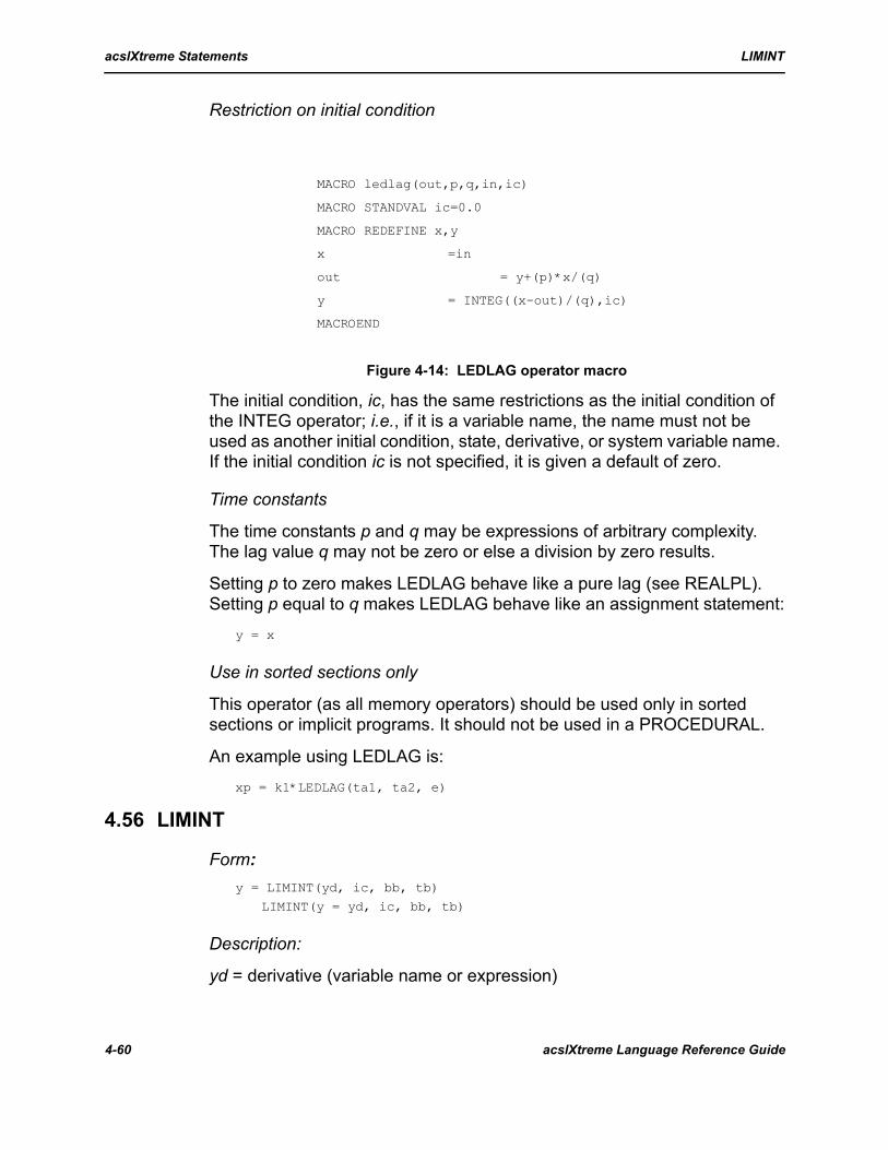
acslXtreme Statements LIMINT
Restriction on initial condition
Figure 4-14: LEDLAG operator macro
The initial condition, ic, has the same restrictions as the initial condition of the INTEG operator; i.e., if it is a variable name, the name must not be used as another initial condition, state, derivative, or system variable name. If the initial condition ic is not specified, it is given a default of zero.
Time constants
The time constants p and q may be expressions of arbitrary complexity. The lag value q may not be zero or else a division by zero results.
Setting p to zero makes LEDLAG behave like a pure lag (see REALPL). Setting p equal to q makes LEDLAG behave like an assignment statement:
y = x
Use in sorted sections only
This operator (as all memory operators) should be used only in sorted sections or implicit programs. It should not be used in a PROCEDURAL.
An example using LEDLAG is:xp = k1*LEDLAG(ta1, ta2, e)
4.56 LIMINT
Form:y = LIMINT(yd, ic, bb, tb)
LIMINT(y = yd, ic, bb, tb)
Description:
yd = derivative (variable name or expression)
MACRO ledlag(out,p,q,in,ic)
MACRO STANDVAL ic=0.0
MACRO REDEFINE x,y
x =in
out = y+(p)*x/(q)
y = INTEG((x-out)/(q),ic)
MACROEND
4-60 acslXtreme Language Reference Guide

acslXtreme Statements LIMINT
ic = initial condition of y, with the same restriction as on the INTEG initial condition (i.e., if it is a variable name, the name must not be used as another initial condition, state, derivative, or system variable name); may be omitted if zero (but comma must be included)
bb = bottom bound on y
tb = top bound on y
Example:
The LIMINT operator could be used as follows:dl = LIMINT(dld, dlic, -dlmx, dlmx)
Figure 4-15: Effect of LIMINT Operator
Use with BOUND
Integrators should not be limited using the BOUND function since the integrator continues to integgrate and then must integrate out of the limit when the derivative changes sign. The LIMINT operaator holds the integrator at the limit as long as the derivative is of such a sign to drive it further into limit. When the derivative reverses sign, the integrator immediately comes off the limit. However, LIMINT and BOUND can be used together to force a hard limit:
y = BOUND(0.0, 1.0, LIMINT(2.0*t, 0.0, 0.0, 1.0))
SCHEDULE alternative
The LIMINT operator can penetrate the limit, especially if the approach is at high velocity (i.e., large values for the derivative and step size). If it is necessary to find the limit points with more precision, use the SCHEDULE operator to force iteration until the limit penetration point is found, then execute a DISCRETE section to set the derivative to zero. Use another SCHEDULE statement to find the point at which the integrator comes back
acslXtreme Language Reference Guide 4-61
acslXtreme Statements LOG
out of the limit and execute another DISCRETE section to begin using the calculated derivative again.
SCHEDULE with LIMINT
The integration routine can be forced to step up to the limit by using SCHEDULE. In this case, the LIMINT operator is used and no DISCRETE section is executed. In the following example, SCHEDULE forces an iteration to the point when X just crosses the symmetric boundary ±xmx.
x = LIMINT(xd, xic, -xmx, xmx)
SCHEDULE .XP. ABS(x)-xmx
Varying the limits
The limits should not vary in time while the system is in the limit.
Use in sorted sections
This operator (as all memory operators) should be used only in sorted sections or implicit programs, and it should not be used in a PROCEDURAL.
4.57 LOG
Form:y = LOG(x)
Description:
The output y is the natural logarithm of x where x is a floating point variable or expression.
Example:
An example using LOG is:y = a - LOG(ABS(SIN(w*t)))
4.58 LOG10
Form: y = LOG10(x)
Description:
The output y is the common logarithm (i.e., to the base 10) of x where x is a floating point variable or expression.
4-62 acslXtreme Language Reference Guide
acslXtreme Statements LOGICAL
Example:
An example using LOG10 is:gdbn = 10.0*LOG10((dlp**2 + dlq**2)*(w/pi*xmag))**2)
4.59 LOGICALSee TYPE.
4.60 LSW, RSW
Form: i = LSW(p, j1, j2)
y = RSW(p, x1, x2)
Description:
Where LSW is the integer switch, and RSW is the real (floating point) switch. The outputs i or y take on the value of the second argument, j1 or x1, when the logical expression p has the value TRUE; otherwise they have the value of the third argument, j2 or x2. The j1 and j2 are any integer expressions; x1 and x1 are floating point expressions. The LSW function is typed INTEGER intrinsically; RSW is floating point.
Example:
Examples of LSW and RSW statements are as follows:INTEGER ncountLOGICAL count
ncount = LSW(count, ncount+1, ncount-1)
cmal = cmalf(mach)*RSW(mach.GT.machmx, (xcg - xcp)/d, 1.0)
Alternative for logicals
For logical switches, assignment statements are simpler and clearer. In the following example, switch is TRUE when x is greater than xmin and FALSE otherwise:
switch = x .GT. xmin
NOTE: All arguments in the statement are evaluated, whether or not they are used. The following statement, therefore, results in an error if p becomes zero:
y = RSW(p .EQ. 0.0, x, x/p)
Writing the statement as follows avoids the problem of division by zero:y = x/RSW(p .EQ. 0.0, 1.0, p)
acslXtreme Language Reference Guide 4-63

acslXtreme Statements MACRO
However, the following solution is preferable because it eliminates an IF statement:
y = x/(p + 1.0E-33)
The probably of p being -1.0E-33 is effectively zero!
4.61 MACRO
Form: MACRO name(x1, x2, ..., xn)
Description:
The keyname MACRO denotes the beginning of a MACRO definition (if not already within a MACRO definition). Within a definition, it denotes special subcommands to be interpreted by the macro processor. For a full description of the macro capability, see Chapter 5.
4.62 MAX
Form: y = MAX(x1, x2, ..., xn)
Description:
The output y is the value of the maximum argument, where the arguments xi are variables or expressions; any number of arguments may be included. Negative values are considered less than positive values.
Example:
The type (INTEGER, REAL, or DOUBLEPRECISION) of the output is implied from the arguments.
nmax = MAX(num1, num2, 2*jj)
w = MAX(wmn, kw*w)
4.63 MAXTERVAL, MINTERVAL
Form: MAXTERVAL name = real constant
Default: name = MAXTreal constant = 1.0E+10
4-64 acslXtreme Language Reference Guide

acslXtreme Statements MAXTERVAL, MINTERVAL
Form:MINTERVAL name = real constant
Default:name = MINT
real constant = 1.0E-10
Description:
Where name is a simple, unsubscripted variable. The maximum and minimum value of the integration step size can be controlled and renamed with these statements.
MAXTERVAL
MAXTERVAL is the upper bound on the integration step size for both variable step and fixed step algorithms.
MINTERVAL
If a variable step size integration algorithm attempts to take a step smaller than the value of the applicable MINTERVAL, the error tag variable (see ERRTAG), if any, is set. If the error tag has already been set, then the termination flag is set. Fixed step algorithms ignore MINTERVAL.
Arrays with multiple sections
If a program contains only one DERIVATIVE section and no DISCRETE sections, MAXTERVAL name (referred to by its default name MAXT hereafter) is a scalar; however, more than one DERIVATIVE and/or DISCRETE section results in MAXT becoming an array. The elements in MAXT then correspond to the sections in the order they are encountered in the source code. If MAXTERVAL is defined outside a DERIVATIVE section, then it is the global default for all DERIVATIVE sections; the elements for DISCRETE sections are ignored. To change MAXT for a specific DERIVATIVE section, put a MAXTERVAL statement with a unique name in the section; for example,
DERIVATIVE
MAXTERVAL maxtsm = 0.0001
The scalar name given is equivalenced to the array element; if the DERIVATIVE section is first in the program, for example, MAXTSM is equivalenced to MAXT(1). At runtime, either the array element or the local name can be referenced.
SET MAXT(1)=0.001SET maxtsm=8.05
acslXtreme Language Reference Guide 4-65
acslXtreme Statements MERROR, XERROR
MINTERVAL is similar, except that for DISCRETE sections the MINTERVAL elements contain the value of the INTERVAL statement; a -1 indicates that there is no INTERVAL statement for the corresponding section.
Integration step size
The integration step size H for fixed step algorithms is calculated from CINT/NSTP (see CINTERVAL and NSTEPS statements) and then bound by MAXT; i.e.,
H = MIN(MAXT, CINT/NSTP)
For variable step algorithms, a lower bound of MINT is added:H = MAX(MINT, MIN(MAXT, CINT/NSTP))
Control of fixed step integration
For fixed step algorithms, we recommend setting NSTP to 1 and MAXT to the desired step size. This approach decouples control of the step size from the communication interval CINT. CINT then is the data logging rate, MAXT is the integration step size, and each can be set separately without affecting the other.
Runtime
The values of these variables can be set by assignment statements in the program or by SET commands at runtime. For example, if the following statement is in a program,
MAXTERVAL MAXT1 = 1.0E-6
then at runtime its value can be changed:SET MAXT1 = 2.0E-6
Even if the MAXTERVAL and MINTERVAL statements are not included in the program, they can be accessed at runtime using the default names of MAXT and MINT. It is seldom necessary to change MINTERVAL.
4.64 MERROR, XERROR
Form: MERROR v1=real constant, v2=real constant, ..., vn
XERROR v1=real constant, v2=real constant, ..., vn
4-66 acslXtreme Language Reference Guide

acslXtreme Statements MIN
Description:
Where MERROR is the relative error bound, XERROR is the absolute error bound, and vi are nonsubscripted variable names that are state variables (i.e., appear on the left side of an INTVC or INTEG statement that is not embedded in an expression). The state itself can be an array, but then the errors specified apply to all elements in the array. Individual elements cannot be given separate error tolerances. If any relative or absolute errors are specified, the first specification encountered is applied to all integrators that are unspecified.
Example:MERROR x=1.0E-4, y=1.0E-6
where:x = INTEG(xd, xic)
y = INTEG(yd, yic)
z = 5.0*INTEG(zzz, 0.0) + COS(x)
Note that z in the above example cannot have any error bounds specified since it is not a state. The actual state is a generated variable name in the Znnnnn form that is placed in the translated assignment statement instead of the INTEG operator. The MERROR and XERROR statements have meaning only for the variable step integration algorithms and are used to limit the error introduced at each step. Based on the maximum absolute value of a state variable |vi |max since the start of the run (a CONTINUE runtime command is considered the start of a run in this context), the allowable error bound is defined to be:
Ei = MAX (Xi, Mi |vi| max)
If any of the predicted errors in an integration step is greater than the corresponding allowable error Ei, the step size is reduced appropriately. If the error is still too large after the step size has been reduced to the minimum (MINTERVAL), the ERRTAG variable, if any, is set TRUE and the run aborted.
For states that are always less than 1.0, the absolute error dominates, which can potentially be a problem. Absolute error is used to cover cases when the variable is near zero. Usually relative error is the important consideration.
4.65 MIN
Form: y = MIN(x1, x2, ... xn)
acslXtreme Language Reference Guide 4-67
acslXtreme Statements MINTERVAL
Description:
The output y is the value of the minimum argument, where arguments xi are variables or expressions. Any number of arguments may be included. Negative values are considered less than positive values.
Example:
The type (INTEGER, REAL, or DOUBLEPRECISION) of the output is inferred from the arguments.
ilo = MIN(imn+1, j, k5) maxtc = MIN(period/nstmn, maxtxz)
4.66 MINTERVALSee MAXTERVAL.
4.67 MOD
Form: y = MOD(x1, x2)
Description:
The output y is the remainder of x1 divided by x2, where x1 and x2 are constants, variables, or expressions. The type (INTEGER or FLOAT) of the function and the output is inferred from the arguments. The generic MOD function is preferred over the more specific AMOD1, MOD0, etc.
The actual implementation can be written as:
x1 =
where [ ] is an integer with magnitude of not more than the argument and with the same sign.
Example:
Examples of MOD are:INTEGER j, k, idiv, icount
icount = 100 + MOD(j*k+100, idiv)
fis = MOD(INTEG(fisd, fisic), twopi)
4.68 NINT
Form: n = NINT(x)
4-68 acslXtreme Language Reference Guide
acslXtreme Statements NSTEPS
Description:
The output y is the nearest integer of x where x is a floating point variable or expression. The output type is always INTEGER. This function differs from INT or AINT, which truncate the input, and from ANINT, which is the nearest whole number with output of type REAL or DOUBLEPRECISION.
Example:
NINT could be used in a subroutine argument list as follows:CALL mysub(NINT(v1), ...)
4.69 NSTEPS
Form: NSTEPS name = integer constant
Default: name: NSTP
integer constant: 10
Description:
Where name is a simple, nonsubscripted variable. The NSTEPS statement defines the integration step size in terms of the communication interval; i.e., NSTEPS is the number of integration steps in a communication interval.
The NSTEPS statement can also be used to rename the variable something different from the default of NSTP.
Type
The variable named in the NSTEPS statement is automatically typed INTEGER.
Variable step algorithms
The effect of NSTEPS with variable step algorithms differs from that with fixed step algorithms. Setting NSTP to a relatively large number is a means of helping a variable step algorithm start at an appropriate size. For variable step algorithms, the step size H is determined by:
H = MAX(MINT, MIN(MAXT, CINT/NSTP))
In other words, the communication interval is divided by NSTP and then the results is bounded by MINT and MAXT. If the first try is too large (i.e., if the estimated error is larger than the allowed error), the algorithm reduces the step size and tries again, until it finds a small enough step size to start off.
acslXtreme Language Reference Guide 4-69
acslXtreme Statements OU
Setting NSTP to a fairly large number (1000, for example) starts the routine at a small step size, which is then increased automatically as the run progresses until it reaches the most efficient size.
NOTE: Beware of leaving NSTP at a large value and switching to a fixed step algorithm.
Fixed step algorithms
For fixed step algorithms (IALG = 3, 4, or 5), MINT is ignored so the step size is calculated by:
H = MIN(MAXT, CINT/NSTP)
We recommend that NSTP be set to 1 so that the integration step size can be controlled by MAXT, specified based on knowledge of the plant dynamics; for example:
NSTEPS nstp1 = 1
MAXTERVAL maxt1 = 0.001
CINTERVAL cint = 0.1
With this procedure, the data logging rate (CINT) is decoupled from the integration step size (now simply MAXT1) so that each can be set independently without affecting the other.
Array of NSTP
When a program contains more than one DERIVATIVE and/or DISCRETE section, NSTEPS becomes an array of length ZZNBLK (the number of sections in the program). The elements of the array correspond to the sections in same order as they appear in the program. For DERIVATIVE sections, each slot contains the appropriate value of NSTEPS, which can be set either globally or else individually for each section. For DISCRETE sections, the slot in NSTEPS is ignored and INTERVAL is used for the step size of any integrations.
4.70 OU
Form: y = OU(t, m, s)
OU(y = t, m, s)
Description:
t= low-pass filter time constant; the break frequency is 1/( (2π τ) Hzm = mean value of ys = standard deviation (RMS value) of y
4-70 acslXtreme Language Reference Guide

acslXtreme Statements OU
The OU operator may be used only in a sorted section or implicit program. It should not be used in a PROCEDURAL. For a random number generator in a nonsorted section, use GAUSS or UNIF.
Band limited white noise is implemented by this Ornstein-Uhlenbeck function. A normal random number generator (GAUSS) delivers a fixed total power (RMS value), but the frequency spread depends on the current step size. Usually the low frequency power density is important, so casual use of GAUSS into a low pass filter leads to ill-defined variation of this quantity as the step size is changed. The Ornstein-Uhlenbeck process maintains a constant source of power over a specified frequency band, thus eliminating any problem of having to include the current integration step size in the standard deviation of the random variable.
NOTE: that in general the roll-off time constant τ should be at least twice the size of the maximum integration step; use MAXTERVAL to enforce this constraint.
The operator is implemented by generating a correlated noise sequence from the general formula:
where:
τ = correlation time constant∆ t =sample intervalωi =Gaussian random variable
In order to find the ωi that produces the correct noise power such that:
square the above equation for n i+1 and take the expected values:
It can be assumed that the random drive is uncorrelated with the noise sequence; i.e.,
But:
so:
and now the sequence can be expressed by
where gi is a Gaussian random variable of zero mean and unit variance. An example using the OU operator is:
ni 1+ nie∆τ– ωi+=
n2 σ2=
nn 1+2 ni
2e 2∆t τ⁄– ω12+=
niωi 0=
ni2 ni
2 1+ σ2= =
ωi2 σ2 1 e 2∆t τ⁄––( )=
ni 1+ nie∆t τ⁄– σ 1 e 2∆t τ⁄––( )gi+=
acslXtreme Language Reference Guide 4-71
acslXtreme Statements PARAMETER
noise = OU(ta1, mean, sigma)
4.71 PARAMETER
Form: PARAMETER(p1 = e1[, p2 = e2] ...)
Description:
The PARAMETER statement associates the symbolic name with an expression that can be made up of constants and/or previously defined parameters but not variables. The symbolic name may then be used whenever an integer, real, logical, or character constant would normally appear in the program code.
Dictionary
The PARAMETER name pi does not appear in the program dictionary and is replaced everywhere by the value of the corresponding expression ei.
Expression
The expression (ei) can consist of literal constants, PARAMETER names, and arithmetic operators (+, -, *, /).
Type INTEGER
PARAMETER variables are not automatically typed INTEGER, even if they begin with letter I, J, K, L, M, or N. Include an INTEGER type statement for any integer PARAMETER variable names before they are used.
Placement in program
The PARAMETER statement must appear in the program before the parameter is used; otherwise, the translator produces an error message:
...Parameter already defined NAME
Example:
PARAMETER statements are useful for defining things like array sizes and for keeping the definitions in one place. For example,
INTEGER maxdim
PARAMETER (maxdim = 5)
DIMENSION a(maxdim,maxdim), v(maxdim), r(maxdim)CONSTANT v = maxdim*1.0
4-72 acslXtreme Language Reference Guide

acslXtreme Statements PROCEDURAL
4.72 PROCEDURAL
Form: PROCEDURAL(output list = input list)
...
END
Description:output list = v1, v2, ..., vn
input list = e1, e2, ..., enand vi
are nonsubscripted variable names while ei may be variables or expressions. The PROCEDURAL header must be paired with a matching END statement.
The PROCEDURAL keyword denotes the beginning of a block of PROCEDURAL code to be executed in the sequence given; i.e., the code within the PROCEDURAL block is not sorted by the acslXtreme translator. PROCEDURAL blocks are required only in sections that are sorted. They are permitted but not required in non-sorted sections of the program.
Arguments
The header list should contain only nonsubscripted variable names. The variable names may belong to arrays, however, in which case the entire array must be filled within the block. The sort algorithm requires that values appear as outputs only once in sorted code; otherwise the error message “Multiply defined symbol” is issued. States and constants do not need to be included in the argument list because they are available all the time. Calculated variables are needed because they tell the sorter where to put the procedural in relation to calculations.
Array example
As an example, the following statements in a sorted program result in the variable A being flagged as defined twice:
a(1) = x + y
a(2) = y + z
This is illegal. An acceptable form would embed this sequence in a PROCEDURAL block, informing the sort routine to place the block before reference to any element of the array A, as follows:
PROCEDURAL(a = x, y, z)
a(1) = x + y
a(2) = y + zEND
acslXtreme Language Reference Guide 4-73
acslXtreme Statements PROCEDURAL
Sorting operation
The entire PROCEDURAL block is moved by the translator within a DERIVATIVE section so that it is placed after the calculation of all variables on the input list and before the use of any variables on the output list. Although other variables may be present on the list, sorting is only with respect to variables calculated within the same DERIVATIVE section. The sort operation never moves code across section boundaries. The entire DERIVATIVE section can be made a PROCEDURAL, and since it then cannot be moved, no input or output argument list is necessary. It is better to use more small PROCEDURALs rather than fewer large ones.
When required
PROCEDURAL blocks should always be used in sorted sections around code constructs in which the order must not be changed. Typical operations which must be enclosed in PROCEDURAL blocks include DO, GO TO, IF, and array calculations. The IF-THEN-ELSE block does not require a PROCEDURAL even in sorted sections.
With subroutine calls
Another construct which may require a PROCEDURAL is the subroutine call. If acslXtreme is not informed which arguments are inputs and which are outputs, a subroutine call may not be sorted correctly. Enclosing subroutine calls in PROCEDURAL blocks or using an equal sign in the subroutine argument list are methods of clarifying input and output lists for the translator (see CALL).
With algebraic loops
Experts may lie in specifying what is on the input/output lists. The acslXtreme translator never looks inside the PROCEDURAL block to ensure compliance with the list supplied, so it is possible to break algebraic loops for approximate solution by omitting one of the loop variables from the PROCEDURAL input list. Since this variable is used before it is calculated, initialization in the INITIAL section is required. In breaking implicit loops this way, the last value of the variable is used, which is satisfactory in a large number of cases. Be warned however that the results change with step size and a variable phase shift is present in traversing the implicit block. This also destroys the validity of the Jacobian and all derived quantities such as eigenvalues, zeros, etc. Use IMPLC to handle algebraic loops.
NOTE: Statements involving memory operators should not be included in PROCEDURAL blocks because parts of these operators must be separated for sorting. These operators are BCKLSH, CMPXPL, DBLINT, DERIVT, LIMINT, and OU.
4-74 acslXtreme Language Reference Guide

acslXtreme Statements PROGRAM
Integration operators
Using integration operators (INTEG, REALPL, etc.) inside PROCEDURAL is not illegal but does not make sense. States cannot be computed procedurally, only derivatives can.
4.73 PROGRAM
Form: PROGRAM [string]
...END
Description:
Where string may contain any number of characters, which are ignored. The PROGRAM statement is the first line in an explicit model definition. It must be accompanied by a matching END statement to terminate the model definition. The character string is not used in any way and serves merely to identify the model file and listing.
Example:PROGRAM a missile 6DOF simulation
For implicit programs (i.e., those with no explicit structure statements), use DERIVATIVE rather than PROGRAM. This approach is required because some system macros have INITIAL sections, which expect explicit structure with the PROGRAM statement. A DERIVATIVE statement can include a name, but for a title with more than one word, use the comment indicator.
DERIVATIVE ! title of program
...END
4.74 PTR
Form: PTR(x, y = r, th)
Description:
The polar to rectangular operator resolves angle θ (which must be expressed in radians) and radius r into Cartesian coordinates x and y (with the same units as r) by the following equations:
x = r cos θ
y = r sin θ
acslXtreme Language Reference Guide 4-75

acslXtreme Statements PULSE
This form is not a functional representation since there are two outputs. Thus, this statement cannot be embedded in an expression; it can only stand alone as shown. Figure 4-16lists the mechanization of this operator as a system macro.
An example of PTR is:PTR(rt1, rt2 = lrt, fi)
Figure 4-16: PTR operator macro
4.75 PULSE
Form: y = PULSE(tz, p, w)
Description:
Where y is a pulse train (0.0 or 1.0) starting at the first integration step at which time equals or exceeds tz. The period is p and width is w, as shown in Figure 4-17. The width cannot be zero.
The independent variable, default T, drives the PULSE function. Note that the integration step size may affect the answers in that too large a step could cause the pulse to seem to stay on indefinitely. The output is always turned on (y = 1.0) at the beginning of the first integration step following the exact turn-on time. The width is not synchronized to the integration step size, so it should be significantly larger than the step size.
Do not use PULSE as a strobe to periodically activate parts of a program. This is a job for DISCRETE sections executed by means of INTERVAL statements or the SCHEDULE operator.
Example:
PULSE could be used as follows:drive = k*PULSE(tdrive, period, width)
MACRO ptr(x1,x2,r,th)
x1 = ®*COS(th)
x2 = ®*SIN(th)
MACROEND
4-76 acslXtreme Language Reference Guide
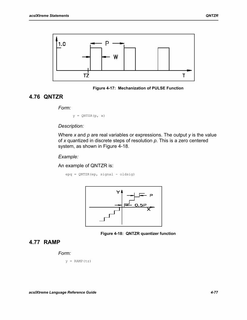
acslXtreme Statements QNTZR
Figure 4-17: Mechanization of PULSE Function
4.76 QNTZR
Form: y = QNTZR(p, x)
Description:
Where x and p are real variables or expressions. The output y is the value of x quantized in discrete steps of resolution p. This is a zero centered system, as shown in Figure 4-18.
Example:
An example of QNTZR is:epq = QNTZR(ep, signal - oldsig)
Figure 4-18: QNTZR quantizer function
4.77 RAMP
Form: y = RAMP(tz)
acslXtreme Language Reference Guide 4-77

acslXtreme Statements REAL
Description:
The RAMP function generates a linear ramp of unit slope, starting at a specified time tz. It is another way of applying a dead zone to the independent variable. RAMP starts at the first integration step that equals or exceeds tz, as depicted in Figure 4-19. The output can be expressed as follows:
y = 0.0 ; T < tz
y = T - tz ; T > tz
Example:
An example of a RAMP statement is:z = k1 + k2*RAMP(tramp)
Figure 4-19: RAMP function
4.78 REAL
Form: REAL(x)
Description:
This function converts an integer, double precision, or single precision argument x to a single precision value. See DBLE for a discussion of usage.
See also REAL as a single precision floating point variable type under TYPE.
4.79 REALPL
Form: y = REALPL(p, x[, ic])
REALPL(y = p, x[, ic])
4-78 acslXtreme Language Reference Guide
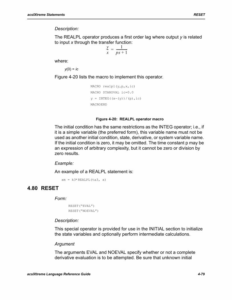
acslXtreme Statements RESET
Description:
The REALPL operator produces a first order lag where output y is related to input x through the transfer function:
where:
y(0) = ic
Figure 4-20 lists the macro to implement this operator.
Figure 4-20: REALPL operator macro
The initial condition has the same restrictions as the INTEG operator; i.e., if it is a simple variable (the preferred form), this variable name must not be used as another initial condition, state, derivative, or system variable name. If the initial condition is zero, it may be omitted. The time constant p may be an expression of arbitrary complexity, but it cannot be zero or division by zero results.
Example:
An example of a REALPL statement is:xm = k3*REALPL(ta3, x)
4.80 RESET
Form: RESET(“EVAL”)
RESET(“NOEVAL”)
Description:
This special operator is provided for use in the INITIAL section to initialize the state variables and optionally perform intermediate calculations.
Argument
The arguments EVAL and NOEVAL specify whether or not a complete derivative evaluation is to be attempted. Be sure that unknown initial
yx-- 1
ps 1+---------------=
MACRO realpl(y,p,x,ic)
MACRO STANDVAL ic=0.0
y = INTEG((x-(y))/(p),ic)
MACROEND
acslXtreme Language Reference Guide 4-79

acslXtreme Statements RSW
conditions have reasonable values to prevent arithmetic errors (division by zero, for example).
When states are initialized
The states are initialized at the beginning of the INITIAL section, the equivalent of RESET(“NOEVAL”). Previously, states had been initialized at the end of the INITIAL section, so there was more reason to use this operator. Now only RESET(“EVAL”) is needed.
Accelerometer example
RESET could be used for example in calculating the initial conditions on accelerometer filters in a missile simulation. To obtain the nominal acceleration, the missile velocity vector must be rotated into the missile axes, the angle of attack determined, and the aerodynamic coefficient data looked up to obtain force coefficients. This code must be expressed in terms of the initial condition variables rather than the state variables unless the RESET operator is used. If the RESET(“EVAL”) statement is placed at the beginning of the INITIAL section, the derivative subroutine calculates body acceleration using the state variable names.
NOTE: The problem in using RESET is that the process is not selective. Calculation of all state variable derivatives is attempted. In the above example, the output of the accelerometer filter is used later and if initialized indefinite leads to an arithmetic error. If the undefined initial conditions are preset in a CONSTANT statement (0.5 is a useful default number), then the calculation can proceed and the meaningless numbers can be disregarded. The important consideration is that all the calculations be able to proceed without arithmetic errors
4.81 RSWSee LSW.
4.82 RTP
Form: RTP(r, th = x, y)
Description:
The rectangular to polar operator resolves the input Cartesian coordinates x and y into polar angle θ (which is in radians in the range − π to + π depending on the magnitude and sign of x and y) and radius r (which has the same units as x and y) by the following equations:
θ = ATAN2 (y, x )
r x2 y2+=
4-80 acslXtreme Language Reference Guide

acslXtreme Statements SAVE
Figure 4-21 shows the mechanization of this operator as a system macro. Note that the second argument of the arc tangent (ATAN2) is modified by the addition of a very small amount. This enables inputs of 0.0, 0.0 to return an angle of zero instead of indefinite.
Figure 4-21: RPT operator macro
This form of the operator is not a functional representation since there are two outputs. Thus, this statement cannot be embedded in an expression; it can be used only in the standalone form as shown.
4.83 SAVE
Form: SAVE
Description:
The macro tables containing the macro names and packed definitions are written (in binary) on the acslXtreme system macro file. The SAVE operation allows you to maintain your own files of macros separate from the system file.
Normally the system reads the contents of the user macro file into the macro definition tables before the translation begins. If such a file does not exist, no user macro definitions are present.
The action of SAVE is to write the current contents of the macro tables back on this file, thus destroying the original contents. To use SAVE, you must have WRITE permission on the current macro file.
4.84 SCALE
Form: SCALE(smn, smx = ymn, ymx)
Description::
ymn, ymx = minimum and maximum values
smn, smx = scaled minimum and maximum to be used on a plot (i.e., rounded multiples of 1, 2, 4, or 10).
MACRO rtp(r,th,x1,x2)
r = SQRT((x1)**2+(x2)**2)
th = ATAN2(x2,x1+1.0e-30)
MACROEND
acslXtreme Language Reference Guide 4-81

acslXtreme Statements SCHEDULE
The SCALE operator rounds the inputs so that they are suitable for plotting. The inputs ymn and ymx are usually collected in the DYNAMIC section by keeping track of the smallest and largest values of the variable of interest. The SCALE operator is then used in the TERMINAL section of an explicit program to establish scale factors for subsequent PLOT commands. It is used only when two or more plots need the same, originally unknown, scale factors.
The first two arguments need not be distinct from the second; i.e., the following statement replaces actual minimum and maximum values with the rounded ones:
SCALE(ymn, ymx = ymn, ymx)
4.85 SCHEDULE
Form: SCHEDULE block/flag .AT. time-expression
SCHEDULE block/flag .XZ. real-expressionSCHEDULE block/flag .XP. real-expression
SCHEDULE block/flag .XN. real-expression
Description::
block = optional block name of DISCRETE section to be executed after the state has been advanced just over the boundary
flag = optional flag name that is automatically made type LOGICAL and set TRUE when the event has occurred (may not be an array)
.AT. = following expression specifies time at which block is to be activated (may not be used in a DERIVATIVE section)
.XZ. = zero crossing (positive or negative direction) of following expression initiates execution of a discrete event.
.XP. = zero crossing (positive direction only) of following expression initiates execution of a discrete event.)
.XN. = zero crossing (negative direction only) of following expression initiates execution of a discrete event.
The block / flag is optional; however, flag cannot be used without a block also being present. SCHEDULE can be used without a block or flag in order to force integration to a certain point.
4-82 acslXtreme Language Reference Guide

acslXtreme Statements SCHEDULE
Flag setting
If a flag is specified, it is set TRUE just before the DISCRETE section is executed, stays TRUE during execution of the section, then is set back to FALSE.
Flag example
The flag is available to handle logic, generally within a single DISCRETE section, as in the following example:
PROGRAM
INITIAL
y = 0.0END ! of Initial
DERIVATIVE
x = SIN(t)SCHEDULE d/f1 .XZ. x+0.5
SCHEDULE d/f2 .XZ. x-0.5
TERMT(t .GE. tstp, ‘Stop on time’);CONSTANT tstp=4.9END
DISCRETE d
IF(f1) THENy = 2.5
ENDIF
IF(f2) THENy =-2.5
ENDIF
END ! of DiscreteEND ! OF Program
Expressions
The time-expression defines a time (real value) of the independent variable at which the event is to be activated. The real-expression defines a function, the zero crossing of which (in the appropriate direction) defines the event. This real-expression must be a true function of the state variables in that the same set of state variables must produce identical values of the function no matter how many intermediate evaluations occur. If the real-expression is not a true function, the following error message may be produced.
Event vanished - cannot proceed
WEDITG
A summary of the activity at the time of an event (i.e., finding and narrowing thewindow and calculating the value of the expression at each evaluation) is produced at runtime at each occurrence of an event. In the example, the event finder is activated in the first line and the window is narrowed over
acslXtreme Language Reference Guide 4-83

acslXtreme Statements SCHEDULE
five iterations. The last two lines of the summary give the values of the independent variable and the zero crossing expression along with the number of the DISCRETE section (i.e., the position of the section among the DERIVATIVE and DISCRETE sections in the program) executed.
This output can be suppressed by setting runtime system symbol WEDITG (write event description, default TRUE) to FALSE.
Handling dicontinues
The SCHEDULE operator handles the introduction of discontinuities into an otherwise continuous simulation. The integration algorithms used to solve equations in the form:
conventionally require the function F to be continuous and differentiable within an integration step. The automatic variable step algorithms such Adams-Moulton or Gear’s Stiff (IALG = 1 or 2) or Fehlberg (IALG = 8 or 9) reduce the step size in the region of a discontinuity in F at the expense of increased processing time, and it is debatable how well the error control mechanism works in the event of a discontinuity in one of the state variables. Nature has no real discontinuities given a sufficiently fine time scale; discontinuities arise from simplifying the model and observing the system behavior in a macro time scale.
Bouncing ball example
In the example of a ball bouncing, the macroscopic view shows the velocity changing discontinuously (by the coefficient of restitution) at the instant of bounce. In the microscopic view, the spring constant of the ball is taken into account and all the forces of deformation are calculated, significantly increasing the model complexity but eliminating the discontinuity.
Digital controller example
Another example is a digital controller. From a macroscopic viewpoint, the output is an analog control voltage through a digital to analog converter (DAC), which jumps discontinuously at the output time points. At a microscopic level, voltages cannot change discontinuously since finite capacitances are always present and must be charged through some sort of resistive network. A simulation normally takes the macroscopic view (i.e., a voltage jump) for efficiency, the designer deciding which time scale of events is important for model validity.
Switch point
If a point of discontinuity can be located, the solution on either side of the discontinuity can be treated as piecewise continuous. A possible penalty is
x· F1 x t,( )=
4-84 acslXtreme Language Reference Guide

acslXtreme Statements SCHEDULE
that the variable step algorithms may have to be restarted after a discontinuity since they keep track of an estimate of derivatives (a Nordsieck1 vector) which is probably invalidated at a switch point.
Time vs. state events
Two types of discontinuity are encountered in general simulation models; one we call a time event and the other a state event. Time events can always be defined as state events, but for efficiency they are extracted as a separate case. State events can be visualized as occurring at surfaces in state space. Such surfaces include the zero height plane in the bouncing ball problem, the zero velocity plane in Coulomb stiction/friction, and the critical temperature plane for a reactor shutdown event. The integration algorithm advances in discrete steps which at some point takes the model across the critical surface; the problem is in finding the exact crossing point.
Finding the event
In the special case of a time event, which is a wall perpendicular to the time axis, the integration step can always be taken as the minimum of the normal step or the time left to the event, so no iteration is required. For state events, where the boundary is a general surface in state space, an iteration brackets the event to a finer and finer tolerance until a specified accuracy is reached. Mathematically the problem is stated:
;;
where the plane in state space distinguishing the event can be expressed by:
g(x, t) = 0
where g is a single-valued function of the state variables and time.
Changing boundaries
In actual fact, the situation can be complicated by the boundary function changing when the state equations switch from F1 to F2. Examples of changing boundaries include backlash, hysteresis, and Coulomb friction. In the friction model, the boundary function is zero velocity when the body is sliding and applied force exceeding breakout force when the body is stuck.
1. Nordsieck, A., “On the Numerical Integration of Ordinary Differential Equations” Math. Comp (1962) pp. 22-49.
x· F1 x t,( )= g x t,( ) 0≥
x· F2 x t,( )= g x t,( ) 0<
acslXtreme Language Reference Guide 4-85

acslXtreme Statements SCHEDULE Time Event Specification
NOTE: State events cannot be scheduled from IF constructs because acslXtreme has to keep a count of the state event statements. Time events can be used inside IF or DO constructs in unsorted sections such as DISCRETE or INITIAL. Multiple IF statements are dangerous; instead, use an IF-THEN-ELSE construct, which covers all the bases so a value is not left around inadvertently.
4.86 SCHEDULE Time Event SpecificationA time event is defined by the .AT. form of the SCHEDULE statement. The time event SCHEDULE must be specified in a DISCRETE section (or in the INITIAL section) and may not be included in a DERIVATIVE section. Every execution of the time event operator places a marker in the event list to execute a block at a particular time. If this were executed in a DERIVATIVE section where the code is executed and re-executed many times under the control of the integration algorithm, the event list would fill with these markers.
A simple example in an INITIAL section to execute DISCRETE switch:INITIAL
CONSTANT swtime = 10.0SCHEDULE switch .AT. swtime
...
END
Execution time
If the value of the time-expression is less than the current time, the block is executed immediately after the current DISCRETE block has finished. Time in the continuous section can never go backwards (with the exception of the entire model moving backwards as described in Chapter 8).
Digital controller example
An example of the use of time events is the modeling of a digital controller with an analog to digital converter (ADC) sampling values from the continuous process, a delay while control output values are computed, and then transfer of these values, usually as voltages through DACs, but also as switch closings to activate solenoids and control valves. For example, for a sampling time of 10 msec and compute delay of 4 msec, the code for the relevant DISCRETE sections could be as follows:
DISCRETE adcINTERVAL tsamp = 0.010
outp = F(sampled inputs)
CONSTANT dlt = 0.004
SCHEDULE dac .AT. T + dltEND ! of adc section
4-86 acslXtreme Language Reference Guide

acslXtreme Statements SCHEDULE Time Event Specification
DISCRETE dac! Executed 4 msec after adc
out = outp
END ! of dac section
The DISCRETE section ADC contains an INTERVAL statement which ensures that the section is executed every 0.010 sec. When it is executed, all the state variables in the continuous section have been advanced to the sampling time, so they are all available as though they had been passed across an ADC channel, except for possible quantization noise. The output can be calculated but must be hidden from the continuous world because it actually comes out of the DAC some time later. In the program, it is hidden by giving it a different name (OUTP). The SCHEDULE statement in the ADC section asks for the DAC time event to be executed at T + 0.004 sec after the ADC section has executed. The DAC block is entered on the event list and control returns to the integration algorithms to advance the continuous state variables until the next event occurs. Time advances the 4 msec and the DAC block is executed, transferring the hidden output variable OUTP into OUT, the name used by the continuous part of the simulation.
No INTERVAL
Since the DISCRETE section DAC has no INTERVAL statement, the only time it is executed is when it is SCHEDULEd from the ADC section.
DISCRETE scheduling itself
As mentioned above, only DISCRETE sections can be scheduled for execution, and time events must be specified within DISCRETE or INITIAL sections. Scheduling time events in DERIVATIVE or DYNAMIC sections results in the same event being scheduled many times (i.e., every time the DERIVATIVE or DISCRETE section is executed). A DISCRETE section can schedule itself for execution in the future, thus replacing the INTERVAL statement.
Event list
All time events are kept on the event list, which is ordered in time. The communication interval for data recording is itself classed as an event and entered on this list. When control is transferred to the continuous integration section, it first checks the event list for the next time event and makes this its goal, advancing with the normal step size selection mechanism until a short step is required to reach the event. When all DERIVATIVE blocks have arrived within the tolerance EPMX (explained in the section on the state event mechanization) of the time event point, the event is deleted from the event list and the associated DISCRETE block (if
acslXtreme Language Reference Guide 4-87

acslXtreme Statements SCHEDULE State Event Specification
any) is executed. The Discrete Sampled Compensator example in Appendix A shows how time events can be used in a digital data system.
4.87 SCHEDULE State Event SpecificationSpecifying an event boundary activates an iteration within the integration algorithm to cross the event boundary with a minimum step size. The forms of SCHEDULE which apply to state events are .XZ. (cross zero), .XP. (cross positive), and .XN. (cross negative). They may appear only in DERIVATIVE sections.
Bouncing ball example
An example of a state event specification is finding the bounce point of a ball dropping (under the acceleration of gravity) with the following statement:
SCHEDULE bounce .XN. h
which executes a DISCRETE block called BOUNCE when height h crosses zero in the negative direction. In the BOUNCE section, velocity is reversed and modified by the coefficient of restitution as follows:
DISCRETE bounce
v = -kr*vEND
Flag vs. multiple DISCRETE
Handling multiple events with a single block usually requires a flag so that the events can be sorted out, but using SCHEDULE operators with separate DISCRETE blocks can remove that requirement.
NOTE: The state event SCHEDULE operator must be placed in a DERIVATIVE section. It may not be placed inside a PROCEDURAL. It may not be skipped over by the use of GO TOs or other control transfer mechanisms (such as the various IF constructs) since acslXtreme needs to keep a count of the SCHEDULE statements. The statement may be placed anywhere in the DERIVATIVE section, but execution is slightly more efficient if it is placed at the beginning of the section since only the code necessary to evaluate the event zero crossing expressions is executed when the time comes to test the event.
4.88 SCHEDULE State Event MechanizationAt the beginning of a simulation run, the DERIVATIVE code is executed. Each call to the state event handler increments a counter so that acslXtreme knows how many events are in operation. If no active state events are present, then there is no need to test for an event at each step. All state SCHEDULE statements must be evaluated at every DERIVATIVE evaluation because they are known by the count of order of appearance.
4-88 acslXtreme Language Reference Guide
acslXtreme Statements SCHEDULE State Event Mechanization
Implementation
After the integration algorithm has been initialized, the integration system saves all the state variables at the beginning of a step, makes the step without regard to any events, and then calls the DERIVATIVE evaluation block one last time to see if the states have crossed the event threshold. Testing is not done during intermediate evaluations of the derivatives since these are extrapolations of much lower accuracy in general than the final step. Since this final evaluation is not part of the evaluation of the derivatives and states (its purpose is only to evaluate the expressions required to execute the DISCRETE block associated with the event), a count is kept and when all expressions corresponding to the state event definitions have been evaluated, then the remainder of the code is skipped. If the expressions are functions of only state variables, the sorter does not have to move them. If they are functions of intermediate calculated quantities (dynamic pressure, for instance), the event specification is sorted to a position just after the calculation of its inputs, thus minimizing the code executed at the threshold test phase.
The first derivative evaluation during the initialization process saves the current value of the real-expression (EXPR) as the previous value (EXPP). At each subsequent step, the current value is tested to see if EXPP and EXPR bracket zero. The code is as follows:
IF(expr*expp .LT. 0 .AND. expp .NE. 0) GO TO event
Starting on zero
Note that if the previous expression EXPP is exactly zero, then no event is signalled. An event is defined as starting from a non-zero value, with the new value crossing or landing exactly on the zero point. An advantage of this method is that the expression can start at zero and no event is indicated until the expression returns to cross zero.
Multiple events
Any number of events can be specified and they all are found in sequence. A crossing point is estimated for each event activated within a step, then the smallest value of the independent variable (time) is selected.
Iterating to step
The iteration within a step proceeds until the zero crossing is within a window less than the tolerance, in which case time is advanced to the most positive edge of the window by calculating the appropriate step size from the saved state condition (at the beginning of the activating step).
acslXtreme Language Reference Guide 4-89

acslXtreme Statements SCHEDULE State Event Mechanization
Executing DISCRETE
Once the step has been taken, the DISCRETE block (if any) associated with each active event is executed so that model conditions can be changed. Usually there is only a single event pending since it is separated in time from other events. However, it is possible that more than one event occurs in the same step and then each associated DISCRETE block (which may be the same one called by different events) is executed in servicing each event.
Re-evalutate DERIVATIVE
After each pending event has been serviced by executing the associated DISCRETE block, the DERIVATIVE routine is executed one last time with a flag set to cause replacement of all previous values (EXPP) with current values. Any current events are thus taken off the active list since the expression must now cross zero from the other side (.XZ.) or return to the other side in order to cross zero from the same direction (.XP.) for the next event.
DISCRETE can change switching function
Note that the execution of the associated DISCRETE block can set variables in such a way as to change the switching function completely. In the case of friction, the switching function fi can be written:
fi = RSW(stuk, ABS(force) - breakf, veloc)
where the function RSW (real switch) returns the value of the second argument if the first argument is TRUE; otherwise, it returns the third argument.
When the body is stuck (STUK is TRUE), the event occurs when the force acting on the body (FORCE) exceeds a breakout force (BREAKF); i.e., when the expression ABS(FORCE) - BREAKF crosses zero. When the body is not stuck, it sticks when the velocity crosses zero. The units of the zero crossing function thus change depending on the regime in which the model stands; i.e., Newtons of force when the body is stuck, and meters per second for velocity when it is not stuck.
Handling discontinuities
Confining discontinuities to the DISCRETE event servicing block is a sound approach. The DERIVATIVE equations can then remain continuous through the event, which allows the event to be found, slopes and states changed, and the integration routine restarted so that past derivative history is discarded.
4-90 acslXtreme Language Reference Guide
acslXtreme Statements SCHEDULE State Event Mechanization
SIGN example
An example of a discontinuity to which the SCHEDULE operator can be applied is the SIGN function. The following statement:
force = SIGN(kslid, -veloc)
indicates that FORCE is to change discontinuously to oppose the velocity, which affects the integration step when the velocity crosses zero. The actual integration step that crosses the boundary has trouble with the discontinuity. In some cases it fails to cross the boundary entirely when the actual step is taken by adding up the weighted intermediate calculated (i.e., fixed step algorithms such as Runge-Kutta fourth order with first order extrapolators). For this case, a better implementation is as follows:
force = fslid
SCHEDULE handl .XZ. veloc
...DISCRETE handl
fslid = SIGN(kslid, -veloc)
END ! of discrete
Now the force is continuous and differentiable (a constant) in the continuous section, giving the integration algorithm an easier task.
NOTE: The event finder also has a problem with the acslXtreme operators which have their own internal memory (or state variables) when it is unable to back up and reproduce the previous step before iterating to find the zero crossing. For example, the backlash operator BCKLSH works by using the statement:
yl = MIN(MAX(yl, input - dl), input + dl)
output = yl
Thus, OUTPUT is the previous value YL (Y last) unless INPUT exceeds YL by more than the backlash value DL. Backing up may leave YL at the same value, so the zero crossing finder may find the expression on the same side of zero after the single step backup, at which point it stops with the message Event vanished. The operators that have internal state variables (potential sources of problems with SCHEDULE) are:
BCKLSH DBLINT DERIVT GAUSS IMPL LIMINT OU UNIF
Operators that are implemented as differential equations (such as REALPL, CMPXPL, and TRAN) have no problem. Algebraic operators (such as STEP and RTP), which pass a signal directly with no memory, also work correctly. DELAY is configured so that it works with SCHEDULE.
First order filter
One workaround for these situations is to put the variable through a first order filter with a fast enough time constant to act the same as a step so the event finder iterates on the continuous (though steep) function. Such a
acslXtreme Language Reference Guide 4-91

acslXtreme Statements Separator (;)
high frequency pole can increase computer running time, however. Another approach is to write a routine to perform the same function using integrators that can be handled by the zero crossing finder.
NOTE: Be careful finding a stopping condition at the boundary since the integration algorithm must take a step that crosses the boundary before recognizing that an event has occurred. To stop on impact with the ground, do not do the following:
SCHEDULE .XN. height
TERMT(height .LE. 0)
The step that makes HEIGHT less than zero also sets the STOP flag so the run is terminated before it can back up and find the zero crossing. Instead use a DISCRETE section; for example:
SCHEDULE stop .XN. height
...END
DISCRETE stop
TERMT(.TRUE., ‘Stopped on zero height’)END
Now the state event iteration takes the step to or just below the HEIGHT equal to zero plane. Then the handler DISCRETE block is executed to set the STOP flag and terminate the run.
4.89 Separator (;)
Form: statement ; statement
Description:
A semi-colon (;) separates any valid acslXtreme statements. Comments can be placed only after the last statement on a line since everything after an exclamation point (!) is ignored by the translator.
Example:TERMT(t.GE.tstop); CONSTANT tstop=4.9 ! Stop Run
4.90 SIGN
Form: y = SIGN(x1, x2)
4-92 acslXtreme Language Reference Guide

acslXtreme Statements SIN
Description:
Where x1 and x2 are floating point constants, variables, or expressions. The output y is the sign of x2 times the absolute value of x1. SIGN could be used as follows:
z = k*SIGN(zbase, zsign)
4.91 SIN
Form: y = SIN(x)
Description:
The output y is the sine of the floating point argument x, which must be in radians; the result is in the range (− 1.0 ≤ y ≤ +1.0).
Example:
SIN could be used:p = INTEG(y*SIN(w*t + fi), 0.0)
4.92 SORT
Form: SORT
Description:
The SORT keyword notifies the translator to sort all statements from the keyword to the end of the section (INITIAL, DYNAMIC, DISCRETE, or TERMINAL). All DERIVATIVE sections are sorted automatically.
This feature could be used for INITIAL sections which have been built from a number of INCLUDE statements without regard to correct order.
4.93 SQRT
Form: y = SQRT(x)
y = SSQRT(x) y = FSQRT(x, lam)
Description:
The output y is the square root of x where x is positive floating point variable or expression. A negative argument results in a exception trap on most computer systems.
acslXtreme Language Reference Guide 4-93

acslXtreme Statements SQRT
Example:
An example using the SQRT function is:miss = SQRT(xmt**2 + ymt**2 + zmt**2)
Alternative functions
Compilers on different systems handle situations such as negative arguments to the square root function differently. In order to catch and handle any errors gracefully, SSQRT (signed square root) and FSQRT (flow square root) functions have been added to the library at Version 11.5. Both convert automatically to single or double precision. The functions are listed in Figure 4-23 and Figure 4-23.
The signed square root function takes the square root of the absolute value of the input, then gives the result the sign of the input. The flow square root function switches to laminar flow when the pressure drop equals the second argument.
Some mathematical models are physically incorrect when the state of the system brings the simulation to the point where it is taking the square root of a negative number. In this case, it should not only use SSQRT to avoid a numerical problem, but also add a TERMT operator to stop the run and report the problem. In some models, flows become zero and noise in the calculations can result in small values on the negative side of zero. In these situations, the BOUND function would probably be used to keep the variable from going negative.
Figure 4-22: Signed Square Root Function (SSQRT)
function ssqrt(dlp)
c-------------------signed square root
c won’t abort when the input becomes negative
c-@@--------------------------single/double
REAL dlp , ssqrt
c
c-------------------use signed root of absolute value
ssqrt = sign(sqrt(abs(dlp)), dlp)
return
end
4-94 acslXtreme Language Reference Guide

acslXtreme Statements STEP
Figure 4-23: Flow Square Root Function (FSQRT)
4.94 STEP
Form: y = STEP(tz)
Description:
The STEP function output y changes from zero to one at a specified value tz of the independent variable. The result is
y = 0.0 ; T < tz
y = 1.0 ; T > tz
function fsqrt(dlp, dlplam)
c-------------------signed square root for flows. has
switch to
c laminar flow when the pressure drop equals the second argument
c the second argument may be zero so that there is
no switch
c to laminar
c
c-@@--------------------------single/double
REAL dlp , dlplam , absdlp , fsqrt
c
c-------------------take absolute value once
bsdlp = abs(dlp)
c-------------------if the absolute value below lami-
nar threshold
c note cannot use equal since possible divide by
zero
if(absdlp .lt. dlplam) then
c-------------------flow is linearly related to pres-
sure drop
fsqrt = dlp/sqrt(dlplam) else
c-------------------use signed root of absolute value
fsqrt = sign(sqrt(absdlp), dlp)
endif
return
end
acslXtreme Language Reference Guide 4-95

acslXtreme Statements TABLE
4.95 TABLE
Form: TABLE name, n, d /list/
Description:
name = name of the function. The value is accessed by name(arg1), name(arg1, arg2), or name(arg1, arg2, arg3) for functions of one, two, or three variables, respectively. The arguments are of any arbitrary level of complexity.
n = an unsigned integer constant giving the number of independent variables; this number must be 1, 2, or 3.
d = unsigned integer constants (may not be variable names); the number of constants must correspond to the value of n. The values of the constants give the number of discrete data points for each successive independent variable. A dimension of one is illegal.
list = floating point constants. The values of the independent variable are listed first. The number of these points must equal the sum of the dimensions. Then the dependent values are listed with the fastest varying argument first. The number of function data points must equal the product of the dimensions.
The TABLE statement describes any arbitrary function of one, two, or three variables. A separate TABLE statement must be used to define each function.
Accessing a TABLE
TABLE statements must be defined before the table is referenced. The table is accessed by name and the independent variable; for example, if CLP has been defined as a table with one independent variable and MACH is a variable calculated previously in the program:
cl = CLP(mach)
Accessing as a function
The table can also be accessed within a statement as with any function:cd(1) = 0.5*CLP(mach)*b*wm(1)/mvm
More than one variable
For a function of more than one variable, the independent variables are all listed in the call, in the order given in the table:
cl = CLP(mach, al)
4-96 acslXtreme Language Reference Guide
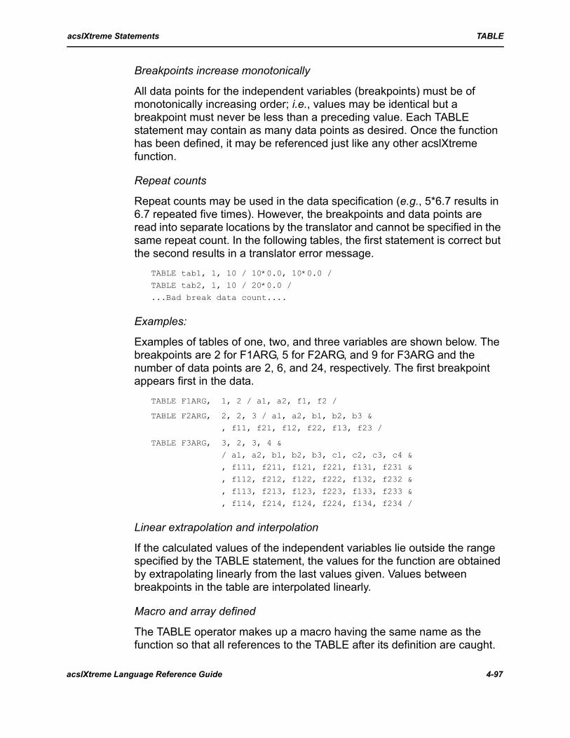
acslXtreme Statements TABLE
Breakpoints increase monotonically
All data points for the independent variables (breakpoints) must be of monotonically increasing order; i.e., values may be identical but a breakpoint must never be less than a preceding value. Each TABLE statement may contain as many data points as desired. Once the function has been defined, it may be referenced just like any other acslXtreme function.
Repeat counts
Repeat counts may be used in the data specification (e.g., 5*6.7 results in 6.7 repeated five times). However, the breakpoints and data points are read into separate locations by the translator and cannot be specified in the same repeat count. In the following tables, the first statement is correct but the second results in a translator error message.
TABLE tab1, 1, 10 / 10*0.0, 10*0.0 /
TABLE tab2, 1, 10 / 20*0.0 /
...Bad break data count....
Examples:
Examples of tables of one, two, and three variables are shown below. The breakpoints are 2 for F1ARG, 5 for F2ARG, and 9 for F3ARG and the number of data points are 2, 6, and 24, respectively. The first breakpoint appears first in the data.
TABLE F1ARG, 1, 2 / a1, a2, f1, f2 /
TABLE F2ARG, 2, 2, 3 / a1, a2, b1, b2, b3 &
, f11, f21, f12, f22, f13, f23 /
TABLE F3ARG, 3, 2, 3, 4 & / a1, a2, b1, b2, b3, c1, c2, c3, c4 &
, f111, f211, f121, f221, f131, f231 &
, f112, f212, f122, f222, f132, f232 & , f113, f213, f123, f223, f133, f233 &
, f114, f214, f124, f224, f134, f234 /
Linear extrapolation and interpolation
If the calculated values of the independent variables lie outside the range specified by the TABLE statement, the values for the function are obtained by extrapolating linearly from the last values given. Values between breakpoints in the table are interpolated linearly.
Macro and array defined
The TABLE operator makes up a macro having the same name as the function so that all references to the TABLE after its definition are caught.
acslXtreme Language Reference Guide 4-97

acslXtreme Statements TABLE
An array is also defined with the same name and enough storage to contain both function data values and the corresponding argument breakpoint values. This array name is entered into the dictionary and it may be accessed in by SET, DISPLAY, etc. runtime commands.
Order of data entry
One point to note is the order of data entry into the array: The function data is listed first, then the breakpoint values follow. This order is the opposite from that listed in the TABLE statement since it was considered that the more normal operation at runtime is changing function values rather than breakpoints. As an example, consider a pitching moment table as a function of Mach number:
TABLE cm, 1, 5 / 0.0, 0.8, 1.2, 1.5, 2.5 &
, 0.50, 0.51, 0.92, 0.83, 0.15 /
This statement produces an array CM(10) in which the first five elements contain the function values 0.50, 0.51, 0.92, 0.83, 0.15 and elements six through ten contain the breakpoint values 0.0, 0.8, 1.2, 1.5, 2.5. To change the function value at Mach 1.5, the following runtime command can be used:
SET cm(4) = 0.65
To change the breakpoint from Mach 1.5 to Mach 1.6, the position in the table is calculated (5 + 4) and the command becomes:
SET CM(9) = 1.6
Multidimensional tables
For multidimensional tables, the function data is all listed in the array first, then the breakpoint data in the order of first, second, third argument.
Function vs. array
The function name followed by parentheses (cm(2.0), for example) on the right hand side of an equal sign implies a call to look up the function value, while the table function name without parentheses stands for the array that contains the function and breakpoint values. The elements of the array cannot be accessed in the program because parentheses indicate a function call, but the array name can be passed to a FORTRAN subroutine (or function) to return the value of the array element. For example, to access the third element of array CM, returned in array value D, call:
CALL getav(cm, 3, d)
where the subroutine is defined at the end of the acslXtreme program:
4-98 acslXtreme Language Reference Guide
acslXtreme Statements TABLE
SUBROUTINE getav(f, n, av)DIMENSION f(1) av = f(n)
RETURN
END
Reading data into array
Data can be read into a TABLE array, either by calling a subroutine within the model or at runtime. Set up the table in the model, but fill the data by using a multiplier; for example:
TABLE k, 1, 10 / 10*0.0, 10*0.0 /
or, if the breakpoints are known and only the data is to be filled in later:
TABLE k, 1, 10 & / 0.0, 0.0, 0.2, 0.4, 0.5, 0.6, 0.8, 0.9, 1.0, 1.0 & , 10*0.0 /
Subroutine call
Thus, to fill a TABLE from outside data, call a subroutine as follows:CALL getk(k, 10)
The subroutine then is defined as follows: SUBROUTINE getk(table, n) REAL table(1)
DATA lu / 55 /
OPEN(UNIT=lu, FILE=’myfile’)C--------------read function values
READ(lu, 99) (table(j), j = 1, n)
C--------------read breakpoint values READ(lu, 99) (table(j), j = n+1, 2*n)
CLOSE(lu)
RETURN 99 FORMAT( < match file data > )
END
Placement of subroutine call
The fill subroutine must appear after the definition of the function by the TABLE statement. If the TABLE statement is specified and a variable with the same name has already been seen, this causes an error.
Since the data needs to be read in only once, the call can be put in the pre-INITIAL section, or else on a switch in the INITIAL section as follows:
acslXtreme Language Reference Guide 4-99
acslXtreme Statements TAN
LOGICAL firstCONSTANT first = .TRUE.
IF(first) CALL getk(k, 10)
first = .FALSE....
4.96 TAN
Form: y = TAN(x)
Description:
The output y is the tangent of the real argument x, which must be expressed in radians.
Example:
TAN could be used as follows:a = b + TAN(theta)
4.97 TERMINAL
Form: TERMINAL
...END
Description:
The TERMINAL keyword identifies the beginning of the block of code performed at the end of each run. It must be paired with a matching END statement. Code in the TERMINAL section is not sorted automatically; however, sorting can be specified with the SORT keyword.
To save calculating certain variables over and over again during the simulation run, the calculations can be placed in the TERMINAL section and executed only at the end of the run.
Multiple TERMINAL sections
Any number of TERMINAL sections can be used within a program. They may appear in any other section (INITIAL, DYNAMIC, DERIVATIVE, and DISCRETE) except PROCEDURAL. This feature is particularly useful in conjunction with INCLUDE files and/or acslXtreme macros. Modules can be developed in separate files with their own TERMINAL sections, then brought into a DERIVATIVE section in a larger program by means of INCLUDE statements.
4-100 acslXtreme Language Reference Guide

acslXtreme Statements TERMT
The translator collects all the TERMINAL sections in the order given. This means that code introduced in DERIVATIVE or DISCRETE sections appears before code in the explicit TERMINAL section. If the sections of code need to be in a particular order (so that a variable is defined before being used, for example), use the SORT keyword.
4.98 TERMT
Form: TERMT(logical expression[, ‘string’])
Description:
A run terminates when the logical expression in the TERMT statement becomes TRUE. Any number of termination conditions may be specified, and the first condition to become TRUE terminates the run.
The ‘string’ argument is an option for printing out user information on the condition that terminates the run. It is considered low volume data and so appears on the screen as well as in the print file. It is useful to include this argument even when there is only one stopping condition since it confirms the run terminating normally.
Example
An example of a typical TERMT statement is:TERMT((h .LE. 0.0) .OR. (v .LE. vmin) .OR. (T .GE. tmax))
or, to provide information at runtime on which condition actually terminated the run:
TERMT(h .LE. 0.0, ‘Termination on hitting ground’)TERMT(v .LE. vmin, ‘Termination on flying backwards’)
TERMT(T .GE. tmax, ‘Termination on TMAX time limit’)
Placement in program
TERMT statements can be placed in any of the DYNAMIC, DERIVATIVE, or DISCRETE sections. A TERMT statement placed in the DYNAMIC section of an explicit program stops the run at a communication interval. In a DERIVATIVE section, it stops the run at the integration step following the logical expression becoming TRUE. In a DISCRETE section, the run stops at the execution following the expression becoming TRUE.
With SCHEDULE
In some cases, a DISCRETE section is executed solely to terminate the run when a state event is detected. For example, SCHEDULE finds the
acslXtreme Language Reference Guide 4-101

acslXtreme Statements TRAN
state event of H (height) crossing zero, and a DISCRETE section contains the TERMT statement:
SCHEDULE stop .XN. h ...
END ! of derivative
DISCRETE stop
TERMT(.TRUE., ‘Termination on hitting ground’)END ! of discrete stop
This procedure is useful for stopping runs at precise events (see, for example, the description of stopping missiles at intercept).
Do not at the same time use an additional statement:TERMT(h .LE. 0.0, ‘Termination on hitting ground’)
For the SCHEDULE operator to work, h must actually cross zero. However, if the statement above is around, it sets the stop flag, thereby stopping the run before SCHEDULE has iterated to find the zero crossing. The result is that the run stops on the other side of the zero crossing rather than precisely on it.
4.99 TRANForm:
y = TRAN(nn, nd, qn, qd, x)TRAN(y = nn, nd, qn, qd, x)
Description:
nn = integer constant or PARAMETER name (may not be a variable name); the order of the numerator polynomial
nd = integer constant or PARAMETER name (may not be a variable name); the order of the denominator polynomial
qn = coefficient array for the numerator (can be an expression); may be a real constant if nn is zero
qd = coefficient array for the denominator
x = input; an arithmetic expression of arbitrary complexity
Transfer functions in the form of a ratio of polynomials in the Laplace operator, s, may be directly implemented by the transfer function simulation operator. The simple first order transfer functions REALPL and LEDLAG and second order CMPXPL should be used when possible since the code generated is more efficient than that for TRAN. TRAN is appropriate for higher order operators.
4-102 acslXtreme Language Reference Guide
acslXtreme Statements TRAN
Order
The transfer function polynomials are in the form of highest power of s coefficient first and any missing order with its coefficient input as zero. Note that nn+1 and nd+1 numbers are required in the numerator and denominator arrays since it is the order that is defined, not the number of coefficients.
NOTE: The order of the denomenator must be greater than or equal to that of the numerator. If the order of the numerator and the order of the denominator are the same and there is a feedback path around the operator, an unsortable statement block may result.
Requirements
All initial conditions are taken as zero, and nn and nd must be literal integer constants or PARAMETER names, but not variable names. Order can be changed by arranging for common factors in the numerator and denominator polynomials. The order cannot be changed artificially by setting the highest power of the denominator polynomial to zero. QD(1) must be nonzero; otherwise division by zero results.
Example
In the following example, note that the s1 term has to be filled in as a zero in the Q (denominator) array. Note also that nn and nd must be entered as the numbers themselves; variable names are not allowed. For the transfer function:
the model code becomes:DIMENSION p(2), q(4)CONSTANT p = 3.0, 2.0, q = 1.0, 2.0, 0.0, 5.0
out = TRAN(1, 3, p, q, in)
Arrays
Variable names as well as literal constants can be used in the arrays. When the numerator is a single value (zero order), it does not need to be declared in an array. Some way of calculating the value (constant, array element, assignment statement, or expression) must be provided, however. For a transfer function in the following form, for example:
only one array is required and the code could be:
G s( ) 3s 2+s3 2s2 5+ +----------------------------=
G s( ) Ks3 1+--------------=
acslXtreme Language Reference Guide 4-103

acslXtreme Statements TRANZ
DIMENSION d(4)CONSTANT d = 1.0, 0.0, 0.0, 1.0
z = TRAN(0, 3, k, d, 5*x + COS(th))
Macro implementation
Figure 4-24 lists the mechanization of the TRAN operator as a system macro. This listing is an example of the complexities that can be implemented using macros.
Figure 4-24: TRAN operator macro
Integration step size
When choosing the integration step size for the model, the reciprocal roots of the denominator polynomial should be considered.
4.100TRANZ
Form: y = TRANZ(nn, nd, qn, qd, x)
TRANZ(y = nn, nd, qn, qd, x)
macro if(nd=1)25do l1 i=2,ndzd(1)=zd(1)-z(i)*q(i+1)l1: zd(i)=z(i-1)macro 25: continuezd(1)=zd(1)/q(1)endmacro decrement nnmacro if(nn=nd)26procedural(out=p,z)macro if(nn=0)30out=p(1)*z(n)macro goto 27macro 26: continueprocedural(out=p,z,zd)out=p(1)*zd(1)macro 27: continuedo l2 i=1,nnl2: out=out+p(i+1)*z(i+n)macro goto 40macro 30: continueout=(p)*z(nd)macro 40: continueendz=intvc(zd,zic)macro exitmacro 999: print Numerator greater than denominator in TRANTRAN: out, nn, nd, p, q, inmacroend
4-104 acslXtreme Language Reference Guide

acslXtreme Statements TRANZ
Description:
nn = integer constant or PARAMETER name (may not be a variable name); the order of the numerator polynomial
nd = integer constant or PARAMETER name (may not be a variable name); the order of the denominator polynomial
qn = coefficient array for the numerator (can be an expression or real constant if nn is zero)
qd = coefficient array for the denominator
x = input; an arithmetic expression of arbitrary complexity
Transfer functions in the form of a ratio of polynomials in Z-1 may be directly implemented in acslXtreme by the TRANZ operator.
Order
The transfer function polynomials are in the form of highest power of Z-1 coefficient first and any missing order with its coefficient input as zero. Note that nn+1 and nd+1 numbers are required in the numerator and denominator arrays since it is the order that is defined, not the number of coefficients. Usually the qd(1) element is unity (1.0).
In the following example, note:
for which the model code becomes:DIMENSION pn(2), qn(3)CONSTANT pn = 1, 0.5
CONSTANT qn = 1,-0.166667,-0.166667
out = TRANZ(1, 2, pn, qn, in)
Coefficients If the number of coefficients in the numerator exceeds those in the denominator, make the denominator order the same as the numerator and fill the trailing coefficients with zeros. When there are no denominator coefficients, use a denominator coefficient array with unity in the first element (qn(1) = 1.0) and the remainder zeros; for example,
DIMENSION pn(4), qn(4)CONSTANT pn = 1, 2, 3, 4
CONSTANT qn = 1, 0, 0 ,0
out = TRANZ(3, 3, pn, qn, in)
matches:
G z( ) 1 0.5z 2–+1 0.166667z 1–– 0.166667z 2––---------------------------------------------------------------------------=
acslXtreme Language Reference Guide 4-105

acslXtreme Statements Type
outn = 1*inn + 2*inn+1 + 3*inn+2 + 4*inn+3
but this is probably better implemented using the HISTORY operator.
Complex filters
For complex Z transform filters, a warning is in order concerning the accuracy of the calculations. It is very easy to come up with a filter design that doesn’t behave correctly and needs double precision in order to work The TRANZ statement must be placed inside a DISCRETE section.
4.101Type
Form: DIMENSION v1, v2, ..., vn
REAL v1, v2, ..., vnDOUBLEPRECISION v1, v2, ..., vnINTEGER v1, v2, ..., vnLOGICAL v1, v2, ..., vnCHARACTER v1*n, v2*n, ..., vn*n
Description:
Where the vi are either simple variable names or else subscripted arrays with up to six integer constant subscripts separated by commas. The variables are typed and (optionally) dimensioned at the same time. Subscripts must be numerical or a symbol defined in a previous PARAMETER statement; variable names are not allowed.
Examples:INTEGER k, jj(10), fred(2, 2)
LOGICAL flag
CHARACTER mytitle*480
REAL x(5,5), k1DOUBLEPRECISION vm(3), dot
Variables are considered to be floating point double precision unless typed otherwise.
LOGICAL
LOGICAL variables can take on values of .TRUE. or .FALSE.
CHARACTER
The length of CHARACTER variables defaults to 1 if not specified.
4-106 acslXtreme Language Reference Guide
acslXtreme Statements Type
Floating point
Variables are cast as DOUBLEPRECISION by default. The variables can be forced to single or double precision by explictly declaring them to be REAL (single precision) or DOUBLEPRECISION.
System symbols
System symbols such as T, CINT, MAXT, and MINT, and also states, derivatives, and initial conditions, are changed automatically by the acslXtreme system and cannot be specified their type.
Duplicates permitted
This is useful in graphic models when declared variables are output from acslXtreme blocks. The variables can be declared in all of the blocks that are wired together, rather than only in the block that computes the variable. Declarations must match exactly, or a diagnostic is produced.
Arguments
A potential problem with mixed single and double precision variables in a program is in their being passed as arguments to subroutines and being returned from functions. All the acslXtreme subroutines change type automatically, but if any other routines are used, provision must be made to force the appropriate type. For example, the DOT product function returns the dot product of two three-component vectors. A total velocity magnitude could be obtained by:
REAL vm(3) mvm = SQRT(DOT(vm,vm))
If DOT is written to accept double precision arguments and return a double precision result, then acslXtreme must type these appropriately rather than relying on automatic typing unless double precision mode is always used:
DOUBLEPRECISION vm(3), DOT
mvm = SQRT(DOT(vm, vm))
If DOT is single precision, the opposite must be specified; i.e.,REAL vm(3), DOT
mvm = SQRT(DOT(vm, vm)
The generic SQRT adjusts automatically to the type of its argument and result.
Literal constants
Other problems occur when using literal constants as arguments to subroutines. For example, quantizing a signal to 0.1 increments could be
acslXtreme Language Reference Guide 4-107

acslXtreme Statements UNIF
written, although it is not good programming practice since the value cannot be changed at runtime.
4.102UNIF
Form: y = UNIF(bb, tb)
Description:
The output y is a random variable uniformly distributed between a bottom bound bb and a top bound tb. UNIF could be used as follows:
drive = k*UNIF(dlo, dhi)
This operator is not intended for use in a DERIVATIVE section because the power density (or, what is usually more important, the low frequency power) depends on the integration step size. Variable step integration methods can produce peculiar results. See OU for details on generating noise in a DERIVATIVE section.
4.103UNIFISee GAUSI.
4.104 VARIABLE
Form: VARIABLE name [, ic name [= floating point constant]]
Description:
The default independent variable is called T. It has an initial value of 0.0 and the initial condition name is not accessible. Using the VARIABLE statement allows you to designate the independent variable with a nonsubscripted name; the initial condition name is then also accessible. The value for the initial condition cannot be a name. If the variable name T is to be used for temperature, for example, the independent variable could be called TIME and be given a negative initial condition as follows:
VARIABLE time, timeic=-5.0
4.105XERRORSee MERROR.
4-108 acslXtreme Language Reference Guide
Macro Language Introduction
Chapter 5 Macro Language
5.1 Introduction Macros are useful for standardizing certain functions for an industry or discipline. Macros can also be used to capture special expertise for other users to incorporate into their programs.
acslXtreme’s language can be expanded using the macro capability to define new operators. These operators are called from the program, usually with arguments. From the macro directives, the translator generates the code (often referred to as macro expansion) for compilation. Code is generated each time the macro is called. Usually the code is slightly different with each call (because of arguments resulting in different variable names, for example).
5.1.1 Macro versus subroutineA macro is similar to a subroutine or function in FORTRAN or procedure or function in C/C++ because it is defined once and then can be invoked as many times and from as many places in the model code as needed. The translator produces a set of statements in the target language compile file for each macro invocation, but the extra storage used for such statements is usually small. Macros are slightly more efficient and have the advantage of being able to define operators involving integrators and memory functions.
Macros are used instead of target language subroutines:
• if any acslXtreme operators are involved• to gain visibility of internal variables• for concatenation to generate unique variables for each application of a macro and
the new variable values are used for printing and plotting.
5.1.2 Macro definitions Macros can be defined:
• in the program in which they are called, before the first invocation.• in a separate program containing only the macros. The program concludes with a
SAVE statement (see the SAVE command in Chapter 4) that saves the macros to the current macro file.
In general, make a local copy of the system macro file and specify this local copy as the macro file for the program to save macro definitions. On some systems, this file must be given WRITE permission. The macro definitions are added to the file (i.e., they are cumulative), so generally it is best to start with a fresh copy of the system macro file. Only translation is required, so stop the acslXtreme build procedure before compilation.
5.1.3 Features Some of the more important features of the macro language are:
acslXtreme Language Reference Guide 5-1

Macro Language Introduction
1. Variables and statement labels may be locally generated. This prevents variables or labels being defined multiple times if the macro is called more than once.
2. The number of macro input arguments is not limited. These arguments must be valid expressions (of arbitrary complexity) with balanced parentheses and any character string enclosed in quotation marks.
3. Macro definitions may invoke other macros to an unlimited level of complexity. However, macro definitions may not be nested because nesting would require a count of the nesting level within the definition to match up with the correct MACRO END. Such a count is not performed and the first MACRO END terminates the definition.
4. Macros may be placed anywhere within an acslXtreme program, but they must be defined before they are used. A macro may be redefined; the most recent version is used in the expansion.
5. The concatenation operator (&) allows arguments to be placed together without intervening spaces, a useful way of making up variable names.
6. Macro definitions can include INITIAL and/or TERMINAL sections.
5.1.4 Forms of call Macros can be called in three ways. The second form, called standalone, is generally preferred because it clearly identifies the usage of MACRO. This makes the statement distinct from subroutine, procedures, and functions. Subroutines or procedures must be invoked using the CALL statement. Function calls return one value and are always in the form of y = func(a,b,c),. The third form must be used with more than one output.
y = MAC(x)
MAC(y = x)MAC(y,z = x)
5.1.5 ConcatenationThe ampersand (&) is the concatenation operator that allows a substitutable argument to appear next to a character string. Its use is discussed in more detail under Macro Definition Header. In general, it enables generation of unique names with multiple calls to a macro. For example, variable V1 is accessed in the following expansion:
MACRO abc(x) y = v&x
MACRO END
abc(1) ...
y = v1
The substituted name must be separated from any other characters by either a space or an ampersand. No substitution would take place in the following situation:
MACRO abc(x)
y = v&xgh
MACRO END
An additional ampersand after the x, however, sets it off so it can be substituted:
5-2 acslXtreme Language Reference Guide
Macro Language Macro definitions
MACRO abc(x) y = v&x&gh
MACRO END
abc(2) ...
y = v2gh
5.1.6 INITIAL, DYNAMIC, DISCRETE, and TERMINAL sections INITIAL, DYNAMIC, DISCRETE, and TERMINAL sections can be used in macro definitions. The translator collects all the code in the order presented (or expanded in the case of macros). These sections are not sorted unless the SORT keyword is specified. Argument strings are substituted for each appearance of the macro argument name. If the argument is an expression, care must be taken that the resulting code is correct after the substitution (see the section on macro calls). Other names that may be substituted during macro expansion are the ASSIGN variable (see MACRO ASSIGN), local variable names identified by a REDEFINE (see MACRO REDEFINE), and local labels identified by a RELABEL (see MACRO RELABEL).
5.2 Macro definitionsThe macro definition is a block of code that consists of:
1) Macro definition header 2) Macro directive or acslXtreme statements 3) MACRO END
The macro definition header specifies the name of the current definition and a list of dummy reference parameters, analogous to dummy arguments in a target language subroutine. The translator scans the statements in the macro body for the appearance of these names, flagging them for substitution by the actual argument supplied on invocation. The definition terminator, MACRO END, must be present to flag the translator to return to direct translation. The translated macro body with arguments substituted is referred to as the skeleton.
If a macro name is the same as one already defined, either in the system macro file or the current model definition, the new macro definition replaces the old one. No error message is issued since this is considered to be a feature whereby you can always override an old macro definition.
5.3 Macro definition header There are two types of macros that can be defined. The first is preferred for most applications send and accept variable names as arguments. The second is useful for handling arrays and can be identified by headers starting MACRO MACRO.
Form: MACRO identifier(x1, x2, ..., xn)
MACRO MACRO identifier(p, q, r, s)
acslXtreme Language Reference Guide 5-3

Macro Language Macro definition header
Description:
identifier = macro name xi = variable names, constants, or expressions p = primary argument specifying an array of input expressionsq, r, and s = secondary arguments giving the names of array dimensionswithin the macro definition.
Arguments p, q, r, and s may be any unsubscripted variable name.
NOTE: If p is the name of the argument of a MACRO MACRO, then a variable named p must not be used in the macro.
5.3.1 First form The first macro form is preferred for most purposes. Anywhere the string of characters xi is referred to in the macro definition, it will be replaced by the ith argument (symbol or expression) when the macro is invoked; e.g.,
MACRO mult(x, y, z) ! definition x = y*z
MACRO END
c = a*mult(5.0*b, d) ! invocation
In this example, the output of the function is the first argument x; but x does not appear explicitly in the invocation. y is replaced by 5.0*B and z by d everywhere throughout the definition.
5.3.2 Second formThe second macro form is useful when handling arrays of indefinite size. This form has an extra MACRO in the header.
The argument p is the dummy reference parameter and may be thought of as a vector, each element of which identifies the respective element in the argument list at invocation time. You specify only p in the invocation. The secondary arguments q, r, and s appear, if needed, in the definition header and may be used in the macro definition, but do not appear in the invocation argument list. Elements of p that are acslXtreme arrays must be dimensioned prior to the macro invocation. Arguments q, r, and s may also be thought of as arrays, but only those elements corresponding to arrays in the p array contain values. They refer to the first, second, and third dimensions, respectively.
MACRO MACRO head(p, q, r, s) ! definition
... definition statements ...
MACRO END DIMENSION b(9), g(2, 3), h(4, 4, 2)
head(a, b = 5*d, e+f, g, h, low) ! invocation
Arguments at invocation time are delimited by either commas or an equal sign. Thus, in this example, p(1) appearing in the definition body is substituted by the symbol a, the first argument, at invocation time. p(4) is replaced by the expression e+f, the fourth argument.
Any reference to q for an array accesses the first dimension. In the example above, q(2) has the value 9 from the dimension of b in the previous DIMENSION statement, but p(1), p(3), p(4), and p(7) are not dimensioned arrays, so q(1), q(3), q(4), and q(7) are scalar have a dimension of one.
5-4 acslXtreme Language Reference Guide

Macro Language Macro directive statements
Symbols substituted for the secondary arguments r and s act similarly to q except they provide the second and third dimensions respectively; for example, r(5) is 3 and s(6) is 2.
Note that macros written in this second form are very hard to read since no mnemonic symbols can be used for the arguments. The array expressions are restricted to the following forms:
1) P(i) where i is a literal integer constant 2) P(n) where n is the ASSIGNed variable 3) P(n±i), combination of the above.
5.3.3 Substitutable symbolsIn general, the substitutable symbols must be separated from other character strings by non alphanumeric characters (i.e., *, +, -, blank) or the concatenation symbol (&) in order for the scan to operate. If the above macro MULT contained the statement:
ASSIGNz TO k
the symbol z would not be identified for substitution. Here the space is all important, so the correct form is the following:
ASSIGN z TO k
5.3.4 ConcatenationThe concatenation operator is the ampersand (&). It is used to allow a substitutable argument to appear next to a character string. It serves as a separator for symbol identification, but is removed when the macro is translated into the skeleton. The following example, shows how to generate unique symbols by adding an F to the third argument of the MULT macro and including it in an expression. The new name would be written F&Z (F concatenated with Z); i.e.,
X = Y*F&Z
Invoking the MULT macro with:
a = mult(sam, joe)
results in the statement:
A = SAM*FJOE
where the new symbol FJOE has been defined. The above call MULT enters a symbol JOE on the symbol table. If only the made up symbols are important, the argument may be quoted using double quotes as:
a = mult(sam, "joe")
In this case, the same expression is generated but now the symbol JOE is not be entered in the symbol table. The argument in double quotes has the quotes removed and the literal string of characters (including any blanks) is substituted for the appropriate argument symbol.
5.4 Macro directive statementsThis section lists alphabetically the macro directive statements that may be included within a macro definition. These statements do not produce code, but can be used to provide
acslXtreme Language Reference Guide 5-5

Macro Language Macro directive statements
extremely flexible control of the macro processing at invocation time. The acslXtreme statements themselves produce code, and symbols in the statements are substituted for the appropriate argument at invocation time. All these directive statements begin with the word MACRO to indicate that they are instructions to the macro processor.
5.4.1 Labels All macro directive statements can have labels attached to them; the labels can be used by MACRO GO TO and MACRO IF directives. These labels must be distinct from any labels attached to non directive statements. The label is inserted after the leading MACRO of the directive; e.g.,
MACRO s1: RELABEL iMACRO s2: CONTINUE
MACRO s3: END
NOTE: These labels control the sequence of the macro processor at macro invocation time. The labels on non directive statements control the sequence at runtime execution.
5.4.2 MACRO ASSIGN
Form: MACRO ASSIGN n
Description:
Where n is a symbol (usually N is used). The ASSIGN directive assigns the number of arguments in the macro call to the variable N; N is always an integer. If the dummy reference parameter contains a variable subscript, the variable must be the same as the variable used in the ASSIGN statement. Whenever N is used as part of the dummy reference parameter subscript, the current value of N refers to the Nth argument in the macro call list at invocation time.
Example:
Using the second header type:
MACRO MACRO sam(P) ! definition MACRO ASSIGN n
... MACRO END
sam(x, y, z) ! invocation
Within the macro definition, N is 3 since the invocation to SAM contains three arguments, and therefore:
p(n) = Nth argument, which is z p(1)(N) = x(3)
p(n-1)(N) = Nth element of the (n-1) argument; i.e., y(3)
5-6 acslXtreme Language Reference Guide

Macro Language Macro directive statements
5.4.3 Arithmetic macro directives
Form:MACRO INCREMENT i
MACRO DECREMENT i
MACRO MULTIPLY i MACRO DIVIDE i
Description:
Where i is an unsigned integer constant, the secondary arguments (p, q, r, s) of the second type of macro, or a macro argument name that has a literal numeric integer value.
These directives provide arithmetic operations on the ASSIGN variable N. The value of N may be added to, subtracted from, multiplied, or divided. All arithmetic operations are performed in fixed point integer.
Example:
MULTIPLY 0 makes the ASSIGN variable zero. To make the ASSIGN variable equal to the dimension of the second argument, the following code can be used:
MACRO MACRO bil(p, q)
MACRO ASSIGN n MACRO MULTIPLY 0
MACRO s1: IF(n = q(2)) s2
MACRO INCREMENT 1 MACRO GO TO s1
MACRO s2: CONTINUE
On exit from this section, N (the assigned variable) has the integer value Q(2), the dimension of the second argument. In this way N can be used as a counter or control variable in addition to its basic purpose of transmitting the number of arguments from the invocation.
5.4.4 MACRO CONTINUE
Form: MACRO CONTINUE
Description:
This macro directive is included so that it can be labeled, as, for example,
MACRO L1: CONTINUE
The MACRO IF or MACRO GO TO can then branch to this section within the definition.
5.4.5 MACRO DECREMENTSee Arithmetic macro directives.
acslXtreme Language Reference Guide 5-7
Macro Language Macro directive statements
5.4.6 MACRO DIVIDE See Arithmetic macro directives.
5.4.7 MACRO EXIT
Form: MACRO EXIT
Description:
The EXIT directive statement stops the generation of code at invocation time. The action is the same as using a MACRO GO TO that transfers control to the macro definition terminator (MACRO END). MACRO EXIT in a PROCEDURAL block can result in translator errors because the END statement will be missing from the PROCEDURAL block.
5.4.8 MACRO GO TO
Form: MACRO GO TO s
Description:
Where s is a statement label attached to another MACRO directive. The GO TO provides an unconditional branch to a labeled macro directive within the definition.
5.4.9 MACRO IF
Form: MACRO IF(e1 = e2) s
Description:
Where s is a macro directive statement label and e1 and e2 can be the dummy reference parameters corresponding to the call list, integer constants, character strings, or the identifier used in the ASSIGN directive. They must not be expressions. The IF directive provides for a conditional branch to the macro directive label s inside the current definition if the relation e1 = e2 holds. The strings e1 and e2 are tested character by character (excluding blanks) for equality. In order to compare a character string with a string passed as a macro argument, the string must be enclosed in quotes when the macro is invoked and then the MACRO IF compares the argument with an un-quote string; i.e., if the definition is as follows:
MACRO test(arg)MACRO IF(arg = top) LAB1
...
MACRO LAB1: CONTINUE
MACRO END
and the invocation is:
5-8 acslXtreme Language Reference Guide
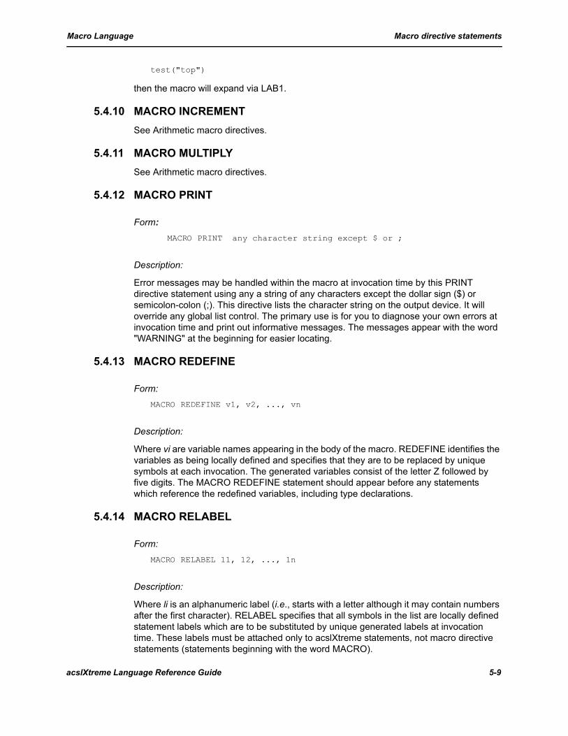
Macro Language Macro directive statements
test("top")
then the macro will expand via LAB1.
5.4.10 MACRO INCREMENT See Arithmetic macro directives.
5.4.11 MACRO MULTIPLY See Arithmetic macro directives.
5.4.12 MACRO PRINT
Form: MACRO PRINT any character string except $ or ;
Description:
Error messages may be handled within the macro at invocation time by this PRINT directive statement using any a string of any characters except the dollar sign ($) or semicolon-colon (;). This directive lists the character string on the output device. It will override any global list control. The primary use is for you to diagnose your own errors at invocation time and print out informative messages. The messages appear with the word "WARNING" at the beginning for easier locating.
5.4.13 MACRO REDEFINE
Form: MACRO REDEFINE v1, v2, ..., vn
Description:
Where vi are variable names appearing in the body of the macro. REDEFINE identifies the variables as being locally defined and specifies that they are to be replaced by unique symbols at each invocation. The generated variables consist of the letter Z followed by five digits. The MACRO REDEFINE statement should appear before any statements which reference the redefined variables, including type declarations.
5.4.14 MACRO RELABEL
Form: MACRO RELABEL 11, 12, ..., 1n
Description:
Where li is an alphanumeric label (i.e., starts with a letter although it may contain numbers after the first character). RELABEL specifies that all symbols in the list are locally defined statement labels which are to be substituted by unique generated labels at invocation time. These labels must be attached only to acslXtreme statements, not macro directive statements (statements beginning with the word MACRO).
acslXtreme Language Reference Guide 5-9

Macro Language Macro directive statements
The following RELABEL statement is illegal because the label name begins with a number:
MACRO RELABEL 110
It could be replaced by the following statement:
MACRO RELABEL L110
To relabel within a macro loop, call another macro from within the loop. For example:
MACRO MACRO test(p) MACRO ASSIGN n
...
MACRO L1: CONTINUE MACRO IF(n=5) L99
mac2(p(n))
MACRO DECREMENT 1 MACRO GO TO L1
MACRO L99: CONTINUE...
MACRO mac2(arg) MACRO RELABEL xyz
MACRO REDEFINE k
DO xyz k=1,25 ... statements that use arg
xyz: CONTINUE
MACRO END
5.4.15 MACRO STANDVAL
Form:MACRO STANDVAL arg1 = c1, arg2 = c2 ...
MACRO STANDVAL P(i) = c1, P(j) = c2, ...
Description:
Where argi are dummy argument names and ci are literal constants that can be real (single or double precision), integer, or logical. In the second form, i and j are unsigned integer constants. The STANDVAL statement is used to provide standard values for arguments of a macro. If the specified argument is not given in the macro call, then the constant is used in its place.
Omitted arguments
If arguments can be omitted from an argument list, they must be at the end of the list.
Placement
The STANDVAL directive must immediately follow the macro header in the definition if it is used at all.
5-10 acslXtreme Language Reference Guide

Macro Language Macro examples
Example:
Several of the acslXtreme operators use this statement. The operator for the second order transfer function (complex pole), for example, begins as follows:
MACRO cmpxpl(y, p, q, x, ic1, ic2)
MACRO STANDVAL ic1=0.0, ic2=0.0
...
A call to this operator in the model source code then need not specify the two initial conditions if they are to be zero:
CMPXPL(y = t1, t2, yp)
5.5 Macro examplesThe following examples of macro calls demonstrate some of the uses of the directive statements and direct parameter substitution.
5.5.1 Sampler A sampler can be created with a switch and two zero order holds. For convenience, the entire sequence can be embedded in a macro and invoked as a function. The invocation could be:
sample(y = dl, x, yic)
When the sampler is repeated for every DL of the independent variable, x is the variable to be sampled, and YIC is the initial value of Y. A macro to handle this could be defined as follows:
MACRO sample(samp, dl, x, ic)
MACRO REDEFINE d, dtINITIAL
samp = ic
ENDDISCRETE d
INTERVAL dt=0.0
dt = dl samp = x
END
MACRO END
Note that the output name must always be included in the argument list. (This requirement for macros is distinguished from target language functions, where the single result is returned into the name of the function.) At the sample time, the DISCRETE section is executed. This action saves the input value x as output value SAMP, which is substituted with the appropriate name from the macro invocation.
5.5.2 Dot product The following call could be used to take the vector dot product of two arrays a and b:
x = DOT(a, b)
acslXtreme Language Reference Guide 5-11
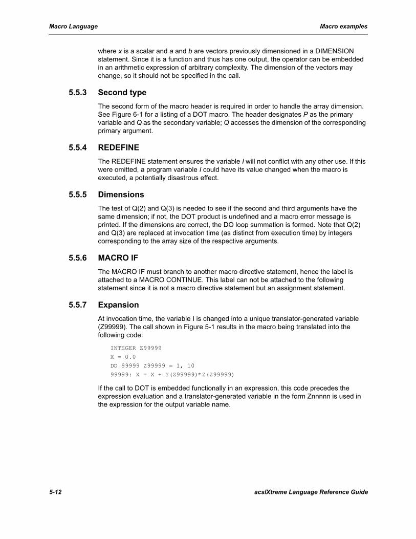
Macro Language Macro examples
where x is a scalar and a and b are vectors previously dimensioned in a DIMENSION statement. Since it is a function and thus has one output, the operator can be embedded in an arithmetic expression of arbitrary complexity. The dimension of the vectors may change, so it should not be specified in the call.
5.5.3 Second typeThe second form of the macro header is required in order to handle the array dimension. See Figure 6-1 for a listing of a DOT macro. The header designates P as the primary variable and Q as the secondary variable; Q accesses the dimension of the corresponding primary argument.
5.5.4 REDEFINEThe REDEFINE statement ensures the variable I will not conflict with any other use. If this were omitted, a program variable I could have its value changed when the macro is executed, a potentially disastrous effect.
5.5.5 Dimensions The test of Q(2) and Q(3) is needed to see if the second and third arguments have the same dimension; if not, the DOT product is undefined and a macro error message is printed. If the dimensions are correct, the DO loop summation is formed. Note that Q(2) and Q(3) are replaced at invocation time (as distinct from execution time) by integers corresponding to the array size of the respective arguments.
5.5.6 MACRO IF The MACRO IF must branch to another macro directive statement, hence the label is attached to a MACRO CONTINUE. This label can not be attached to the following statement since it is not a macro directive statement but an assignment statement.
5.5.7 Expansion At invocation time, the variable I is changed into a unique translator-generated variable (Z99999). The call shown in Figure 5-1 results in the macro being translated into the following code:
INTEGER Z99999 X = 0.0
DO 99999 Z99999 = 1, 10
99999: X = X + Y(Z99999)*Z(Z99999)
If the call to DOT is embedded functionally in an expression, this code precedes the expression evaluation and a translator-generated variable in the form Znnnnn is used in the expression for the output variable name.
5-12 acslXtreme Language Reference Guide
Macro Language Macro examples
Figure 5-1: DOT product macro and invocation
5.5.8 Pressure tank This pressure tank example illustrates the use of concatenation in macros. A similar example (physiological benchmark PHYSBE) appears in Appendix A.
5.5.9 Concatenation One of the problems with using macros is the tendency to generate large numbers of dummy variables (Znnnnn) which have no mnemonic meaning. All REDEFINEd variables have this form. An alternate approach is to use the concatenation feature to build unique symbols that are available for plotting or printing. This technique can also reduce considerably the length of the argument list; using a long argument list is the other alternative when unique symbolic names are required.
5.5.10 DefinitionIn this example, a macro is defined for a gas holding tank. The flow into the tank is calculated as the difference in pressure divided by a resistance. Total pressure is the integrated net flow divided by a volume. The macro definition is thus:
MACRO tank(n)f&n&i = (p&n&i - p&n)/r&n&i
p&n = (INTEG((f&n&i - f&n&o)/v&n, p&n&ic)
MACRO END
5.5.11 InvocationThe basic equations for different vessels (tank 1 and tank 3, for example) can now be established in the model by the statements:
tank(1) tank(3)
5.5.12 Expansion The invocation TANK(3), for example, generates the following translated code:
MACRO MACRO dot(p, q) MACRO RELABEL loop MACRO REDEFINE i MACRO IF(q(2)=q(3)) ml1 MACRO PRINT Conflicting dimensions in dot product MACRO EXIT MACRO ml1: CONTINUE PROCEDURAL(p(1) = p(2), p(3)) p(1) = 0.0 DO loop i = 1, q(2) p(1) = p(1) + p(2)(i)*p(3)(i) loop: continueEND ! of procedural MACRO END ! Invocation of dot macro DIMENSION y(10), z(10) dot(x = y, z)
acslXtreme Language Reference Guide 5-13

Macro Language Macro examples
F3I = (P3I - P3)/R3I P3 = INTEG((F3I - F30)/V3, P3IC)
5.5.13 Constants and variables Constants must be defined elsewhere for the resistance R3I, the volume V3, and initial pressure P3IC. Variables which must be defined elsewhere are the input pressure node P3I and the output flow F3O. This macro then makes available to other sections of the simulation the input flow F3I and tank pressure P3.
5.5.14 Alternative form An alternative form of the macro invocation without the concatenation feature would have to be a separate statement such as the following for each tank in the system:
tank(f3i, p3 = p3i, r3i, f3o, v3, p3ic)
5.5.15 Advantages of concatenationThe trade-off in deciding how to define the macro can be stated generally as follows: Without the concatenation feature, argument lists become long and complicated, but argument lists have the advantage of flexibility in naming; in addition, arguments can be expressions. Using the concatenation feature, the argument list is simple: one argument (usually a literal constant, but can an alphanumeric variable name). An alternative TANK macro could have the output flow and downstream pressure specified in the argument list since these are likely to be expressions; e.g.,
MACRO tank(n, pi, fo)f&n&i = (pi - p&n)/r&n&i
p&n = INTEG((f&n&i - (fo))/v&n, p&n&ic)
MACRO END
The invocation of this macro could, for example, substitute a variable name for inlet pressure PI and an expression for the outlet flow FO, as follows:
tank(1, psource, (p1 - p5)/r51)
The disadvantage of the concatenation approach is the inflexibility in naming convention, but if you have control of the model design, you can use this to advantage.
5.5.16 Matrix operations Matrix operations such as addition, multiplication, negation, and transposition can be defined by macros. Macros for these four operations are listed in Figures 6-2 through 6-5 and the macro for matrix multiply (MMUL) is discussed in detail.
Note that matrix operations are usually characterized by an n-cubed operation count and can be expensive for large matrices.
5-14 acslXtreme Language Reference Guide
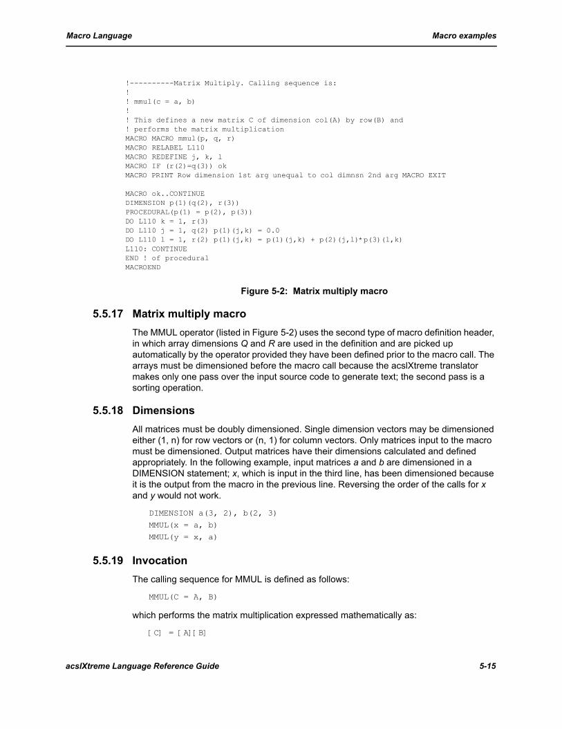
Macro Language Macro examples
Figure 5-2: Matrix multiply macro
5.5.17 Matrix multiply macro The MMUL operator (listed in Figure 5-2) uses the second type of macro definition header, in which array dimensions Q and R are used in the definition and are picked up automatically by the operator provided they have been defined prior to the macro call. The arrays must be dimensioned before the macro call because the acslXtreme translator makes only one pass over the input source code to generate text; the second pass is a sorting operation.
5.5.18 DimensionsAll matrices must be doubly dimensioned. Single dimension vectors may be dimensioned either (1, n) for row vectors or (n, 1) for column vectors. Only matrices input to the macro must be dimensioned. Output matrices have their dimensions calculated and defined appropriately. In the following example, input matrices a and b are dimensioned in a DIMENSION statement; x, which is input in the third line, has been dimensioned because it is the output from the macro in the previous line. Reversing the order of the calls for x and y would not work.
DIMENSION a(3, 2), b(2, 3) MMUL(x = a, b)
MMUL(y = x, a)
5.5.19 Invocation The calling sequence for MMUL is defined as follows:
MMUL(C = A, B)
which performs the matrix multiplication expressed mathematically as:
[C] = [A][B]
!----------Matrix Multiply. Calling sequence is: !! mmul(c = a, b) ! ! This defines a new matrix C of dimension col(A) by row(B) and ! performs the matrix multiplication MACRO MACRO mmul(p, q, r) MACRO RELABEL L110 MACRO REDEFINE j, k, l MACRO IF (r(2)=q(3)) ok MACRO PRINT Row dimension 1st arg unequal to col dimnsn 2nd arg MACRO EXIT
MACRO ok..CONTINUE DIMENSION p(1)(q(2), r(3)) PROCEDURAL(p(1) = p(2), p(3)) DO L110 k = 1, r(3) DO L110 j = 1, q(2) p(1)(j,k) = 0.0 DO L110 l = 1, r(2) p(1)(j,k) = p(1)(j,k) + p(2)(j,l)*p(3)(l,k)L110: CONTINUE END ! of procedural MACROEND
acslXtreme Language Reference Guide 5-15
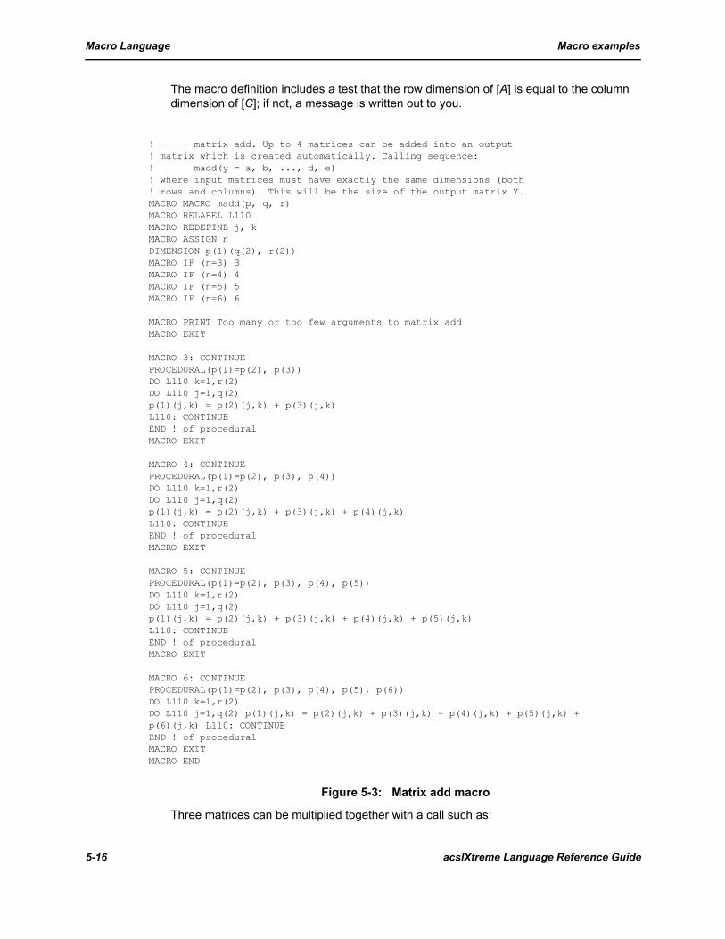
Macro Language Macro examples
The macro definition includes a test that the row dimension of [A] is equal to the column dimension of [C]; if not, a message is written out to you.
Figure 5-3: Matrix add macro
Three matrices can be multiplied together with a call such as:
! - - - matrix add. Up to 4 matrices can be added into an output ! matrix which is created automatically. Calling sequence: ! madd(y = a, b, ..., d, e) ! where input matrices must have exactly the same dimensions (both ! rows and columns). This will be the size of the output matrix Y.MACRO MACRO madd(p, q, r) MACRO RELABEL L110 MACRO REDEFINE j, k MACRO ASSIGN n DIMENSION p(1)(q(2), r(2)) MACRO IF (n=3) 3 MACRO IF (n=4) 4 MACRO IF (n=5) 5 MACRO IF (n=6) 6
MACRO PRINT Too many or too few arguments to matrix add MACRO EXIT
MACRO 3: CONTINUE PROCEDURAL(p(1)=p(2), p(3)) DO L110 k=1,r(2) DO L110 j=1,q(2) p(1)(j,k) = p(2)(j,k) + p(3)(j,k) L110: CONTINUE END ! of procedural MACRO EXIT
MACRO 4: CONTINUE PROCEDURAL(p(1)=p(2), p(3), p(4)) DO L110 k=1,r(2) DO L110 j=1,q(2) p(1)(j,k) = p(2)(j,k) + p(3)(j,k) + p(4)(j,k) L110: CONTINUE END ! of procedural MACRO EXIT
MACRO 5: CONTINUE PROCEDURAL(p(1)=p(2), p(3), p(4), p(5)) DO L110 k=1,r(2) DO L110 j=1,q(2) p(1)(j,k) = p(2)(j,k) + p(3)(j,k) + p(4)(j,k) + p(5)(j,k) L110: CONTINUE END ! of procedural MACRO EXIT
MACRO 6: CONTINUE PROCEDURAL(p(1)=p(2), p(3), p(4), p(5), p(6)) DO L110 k=1,r(2) DO L110 j=1,q(2) p(1)(j,k) = p(2)(j,k) + p(3)(j,k) + p(4)(j,k) + p(5)(j,k) + p(6)(j,k) L110: CONTINUE END ! of procedural MACRO EXIT MACRO END
5-16 acslXtreme Language Reference Guide
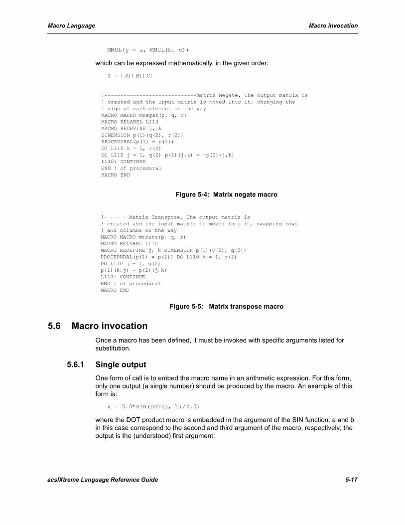
Macro Language Macro invocation
MMUL(y = a, MMUL(b, c))
which can be expressed mathematically, in the given order:
Y = [A][B][C]
Figure 5-4: Matrix negate macro
Figure 5-5: Matrix transpose macro
5.6 Macro invocation Once a macro has been defined, it must be invoked with specific arguments listed for substitution.
5.6.1 Single output One form of call is to embed the macro name in an arithmetic expression. For this form, only one output (a single number) should be produced by the macro. An example of this form is:
x = 5.0*SIN(DOT(a, b)/4.0)
where the DOT product macro is embedded in the argument of the SIN function. a and b in this case correspond to the second and third argument of the macro, respectively; the output is the (understood) first argument.
!-----------------------------Matrix Negate. The output matrix is ! created and the input matrix is moved into it, changing the ! sign of each element on the way MACRO MACRO mnegat(p, q, r) MACRO RELABEL L110 MACRO REDEFINE j, k DIMENSION p(1)(q(2), r(2)) PROCEDURAL(p(1) = p(2)) DO L110 k = 1, r(2) DO L110 j = 1, q(2) p(1)(j,k) = -p(2)(j,k) L110: CONTINUE END ! of procedural MACRO END
!- - - - Matrix Transpose. The output matrix is ! created and the input matrix is moved into it, swapping rows ! and columns on the way MACRO MACRO mtrans(p, q, r) MACRO RELABEL L110 MACRO REDEFINE j, k DIMENSION p(1)(r(2), q(2)) PROCEDURAL(p(1) = p(2)) DO L110 k = 1, r(2) DO L110 j = 1, q(2) p(1)(k,j) = p(2)(j,k) L110: CONTINUE END ! of procedural MACRO END
acslXtreme Language Reference Guide 5-17

Macro Language Macro invocation
5.6.2 Standalone formsAn alternative form of the call is as a standalone statement, which has two forms as follows:
DOT(x = a, b)
DOT(x, a, b)
The equal sign in the first form is to indicate to the reader that x is an output. The program determines the actual inputs and outputs as it processes the statements produced by the macro; i.e., no error would result if the operator were invoked as follows:
DOT(x, a = b)
but it would be misleading to the user. Note especially that
x = DOT(a, b)
is an assignment statement and the name x is not substituted for the first argument. Only a single numerical value can be passed across the equal sign of an assignment statement.
On the other hand, consider a matrix integration operator which might be invoked as follows:
matint(x, xd = a, xic)
In this call, two entire vectors are the output of the operator and have their values effectively passed across the equal sign. Passing more than one value across an equal sign is possible only in macro and subroutine calls.
5.6.3 Argument substitutionThe substitution of macro arguments is by replacement of the character string forming the argument with the substitutable name. Where expressions are used, the wrong answer can be obtained if parentheses are not placed around the argument. For example, consider a macro to integrate a difference in flow rate as follows:
MACRO accum(tot, w1, w2, ic)
tot = INTEG(w1 - w2, ic) MACRO END
At invocation, an expression for net flow out becomes:
accum(mass = win, wp1 + wp2, massic)
which produces the line of code:
MASS = INTEG(WIN - WP1 + WP2, MASSIC)
5.6.4 Use of parenthesesThis result is not exactly right, since the second flow WP2 has been made positive. The solution, when the operator precedence can cause a problem, is to surround the substitutable name with parentheses. The macro above should have been defined as follows:
5-18 acslXtreme Language Reference Guide
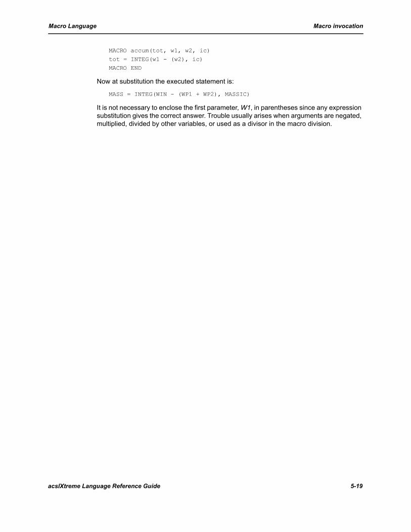
Macro Language Macro invocation
MACRO accum(tot, w1, w2, ic) tot = INTEG(w1 - (w2), ic)
MACRO END
Now at substitution the executed statement is:
MASS = INTEG(WIN - (WP1 + WP2), MASSIC)
It is not necessary to enclose the first parameter, W1, in parentheses since any expression substitution gives the correct answer. Trouble usually arises when arguments are negated, multiplied, divided by other variables, or used as a divisor in the macro division.
acslXtreme Language Reference Guide 5-19

Macro Language Macro invocation
5-20 acslXtreme Language Reference Guide

Appendix A Programming Style
A.1 Why care about programming style?The Golden Rule of programming is:
Document unto others as you would have them document unto you.
This section suggests some guidelines for making acslXtreme programs more readable, which leads to fewer errors and better documentation. The elements of programming style include program layout (physical appearance, including numerous comments), units (using consistent units throughout the program), naming conventions (to make name recognition easy), and a program dictionary that can be maintained as the program develops.
A.2 Program LayoutReadability is greatly enhanced by a neat, consistent layout with columnar organization and spaces. Almost any thoughtful layout does the job.
A.2.1 TemplateTemplates can save programming time and encourage uniformity. Templates can be as simple or as elaborate as required. A file called TEMPLATE.CSL (see Figure A-1) is distributed with acslXtreme. This is an outline of the explicit acslXtreme structure plus the system symbols for program control.
Figure A-1: Template File TEMPLATE.CSL
PROGRAM name
INITIAL ? END ! of initial
DYNAMIC
ALGORITHM IALG = ? NSTEPS NSTP = ? MAXTERVAL MAXT = ? MINTERVAL MINT = ? CINTERVAL CINT = ?
DERIVATIVE ? END ! of derivative
CONSTANT TSTOP = ? TERMT( T .GE. TSTOP ) ?END ! of dynamic
TERMINAL ?END ! of terminal
END ! of program
A-1 acslXtreme Language Reference Guide

A.2.2 OriginatorSpecifying the originator’s name and location serves as a point of contact. Expressing dates in the form dd MMM yyyy avoids the ambiguity of mm/dd/yy or dd/mm/yy or yy/mm/dd.
! John Doe and Jane Roe
! ABCDE Inc., Washing Engineering Division
! 09 JULY 1999
A.2.3 DescriptionA brief statement of the purpose and general structure of the program helps quickly identify the program.
! Simulation of a hydraulic valve for the XYZ actuator ! Inputs: PI (input pressure) and A1 (aperture)
! Outputs: V0 (volume of fluid output)
! Units: m-kg-sec
A.2.4 Statement layoutCSL in acslXtreme is free form. There are no restrictions on line length, or the need to place characters in any particular column. For example, the continuation character, the ampersand (&), can be placed where the user wants to end the line.
A.2.5 Program structureThe program structure keywords (PROGRAM, INITIAL, DYNAMIC, DERIVATIVE, DISCRETE, TERMINAL, and their matching ENDs) are the largest structures in the program. Therefore it helps to start them in column 1 where they can be easily found. Appending comments to the END statements (Figure A-1) helps keep track of them.
A.2.6 Assignment statementsLining up the equal signs helps when scanning listings. Spaces precede and follow the equal sign, except when a minus sign follows the equal sign. Signs can be critical in simulations, and the extra visibility of the minus signs helps avoid errors.
sam = a + b
array(i, j, name) = velocsth = x/(h + y1)
xdd = -2.0*fk1*sth/m1
A.2.7 OperatorsOperators (including logical operators) are more visible with spaces on both sides of them. Because of mathematical convention rather than any programming restriction, multiplication (*), division (/), and exponentiation (**) operators are not spaced.
A(J,K) = X*Y + SIN(2.0*X - AL)
Y = SQRT(X**2 + Z**2)/GIF(C .EQ. D) CALL SUBR
A-2 acslXtreme Language Reference Guide

A.2.8 CommasA comma is followed by a space for greater readability. In general, no space precedes it unless called for by layout specification in lists.
CALL subr (a + b, SIN(x), y)
A.2.9 ParenthesesParentheses generally do not use spaces, especially not between a subroutine or function call and its arguments.
CALL subx(x, y, aout)
y = dot(x, z)
A.2.10 ContinuationPutting an ampersand (&) at the end of the line, continues it onto another line. Break the statement at a logical place in the expression.
TABLE clp, 1, 5 & / 0.0 , 0.8 , 1.0 , 1.2 , 2/0 &
,-0.21 , -0.21 ,-0.20 ,-0.19 , -0.18 /
cl = clz + clal*al + clde*dle & , + (cb/(2*v))*(clad*ald + cltd*q)
An ampersand at the beginning of the continuation line eliminates blanks. This is useful when a name or a character string carries over the line.
charactervariable = ‘longcharact&
&erstring’
A.2.11 ListsDimension (DIMENSION) lists, type lists (REAL, INTEGER, LOGICAL) and CONSTANT statements are easier to read if they are lined up in columns; for example:
DIMENSION nm(3) , vm(3) , rm(3)INTEGER count , i , k
LOGICAL flag , switch
CONSTANT k1=2.0 , k2 = 10.0 , kact1=5455.0CONSTANT damp = 0.1
A.2.12 Comments (!)A line of dashes aids the eye in finding comments easily. Blank lines are better for the end of large logically connected sequences of code.
!------------This is a short comment.
!------------This is a longer comment.
! continued on a second line.
acslXtreme Language Reference Guide A-3
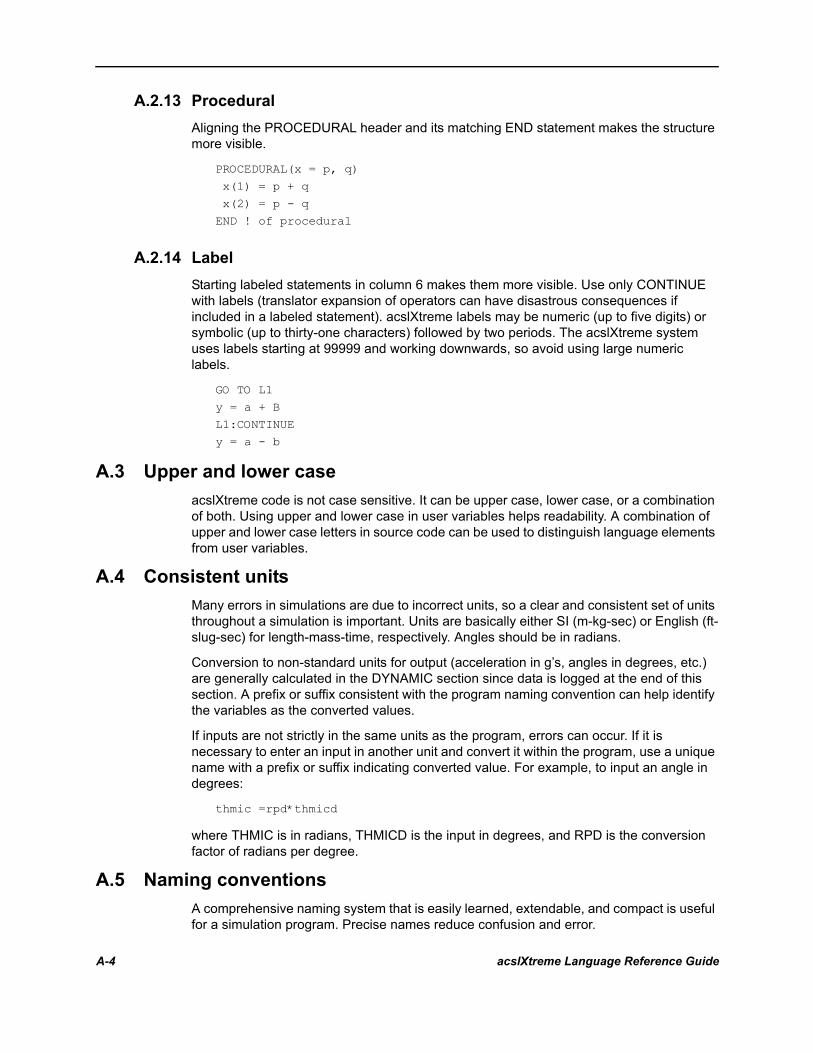
A.2.13 ProceduralAligning the PROCEDURAL header and its matching END statement makes the structure more visible.
PROCEDURAL(x = p, q)
x(1) = p + q
x(2) = p - q
END ! of procedural
A.2.14 LabelStarting labeled statements in column 6 makes them more visible. Use only CONTINUE with labels (translator expansion of operators can have disastrous consequences if included in a labeled statement). acslXtreme labels may be numeric (up to five digits) or symbolic (up to thirty-one characters) followed by two periods. The acslXtreme system uses labels starting at 99999 and working downwards, so avoid using large numeric labels.
GO TO L1
y = a + B
L1:CONTINUEy = a - b
A.3 Upper and lower caseacslXtreme code is not case sensitive. It can be upper case, lower case, or a combination of both. Using upper and lower case in user variables helps readability. A combination of upper and lower case letters in source code can be used to distinguish language elements from user variables.
A.4 Consistent unitsMany errors in simulations are due to incorrect units, so a clear and consistent set of units throughout a simulation is important. Units are basically either SI (m-kg-sec) or English (ft-slug-sec) for length-mass-time, respectively. Angles should be in radians.
Conversion to non-standard units for output (acceleration in g’s, angles in degrees, etc.) are generally calculated in the DYNAMIC section since data is logged at the end of this section. A prefix or suffix consistent with the program naming convention can help identify the variables as the converted values.
If inputs are not strictly in the same units as the program, errors can occur. If it is necessary to enter an input in another unit and convert it within the program, use a unique name with a prefix or suffix indicating converted value. For example, to input an angle in degrees:
thmic =rpd*thmicd
where THMIC is in radians, THMICD is the input in degrees, and RPD is the conversion factor of radians per degree.
A.5 Naming conventionsA comprehensive naming system that is easily learned, extendable, and compact is useful for a simulation program. Precise names reduce confusion and error.
A-4 acslXtreme Language Reference Guide

A.5.1 Name lengthThe length of variable names is determined by the target code compiler. Thirty-one alpha-numeric characters is a general standard. Short names are usually easier to read, quicker to type, and less likely to be misspelled. Names should not be too short, because one and two character names have a high possibility of conflict and locating them with an editor is sometimes difficult.
A.5.2 Greek lettersA convention for Greek symbols can help in standardizing code. A suggested standard using two-characters mnemonics is shown in Table A-1. The exception to the two-character designation is W for omega.
A.5.3 Object characters, action characters, and modifiersA concept which can be helpful in constructing meaningful variable names is the idea of object characters, action characters, and modifiers. The terms and characters would be specialized to a particular field. In the aerospace field, for example, typical object characters might be: E (earth), M (missile), T (target), P (autopilot), G (gimbal), and H (head). Action characters might be: R (range), V (velocity), A (acceleration), W (angular rate), F (force), and M (moment). The action character appears first in the name; thus, the range of the missile is RM, the velocity of the target is VT, etc.
Modifiers are either prefixes or suffixes to the action-object names. Derivatives, for example, can be indicated with suffix D; a double derivative, with DD, etc. Other suffixes might be: IC (initial condition), MN (minimum), MX (maximum), P (previous), and Z (nominal value). Letters designating reference frames can also be used as suffixes when variables are transformed from one frame to another. Prefixes can be indications of the type of variable, e.g., S (sine), C (cosine), A (absolute value), L (vector length), M (measured), E (estimated), U (unit vector), and X (converted).
Direction is important in many systems, especially mechanical systems. To keep directions clear, variables are usually expressed as vectors in terms of reference frames, with values positive along the associated axes. Vector components can be identified by axis number (i.e. RM(1), RM(2), and RM(3)); this approach allows the vector to be handled as a unit for integration, rotation, and addition. Angles, rates, moments, etc. are usually positive by the right-hand rule about the respective axes.
α alpha AL ι iota IO ρ rho RO
β beta BE κ kappa KA σ sigma SG
γ gamma GA λ lambda LA τ tau TA
δ delta DL µ mu MU υ upsilon UP
ε epsilon EP ν nu NU ϕ phi FI
ζ zeta ZE ξ xi XI χ chi CH
η eta ET ο omicron ON ψ psi SI
θ theta TH π pi PI ω omega W
Table A-1: Suggested Greek Symbol Names
acslXtreme Language Reference Guide A-5

Relative vectors can be expressed with two subscripts, in the order they appear on the right side of the equation. For example, the range to the target from the missile is:
rtm = rt - rm
These concepts can be adapted for a particular industry or simulation system.
A-6 acslXtreme Language Reference Guide
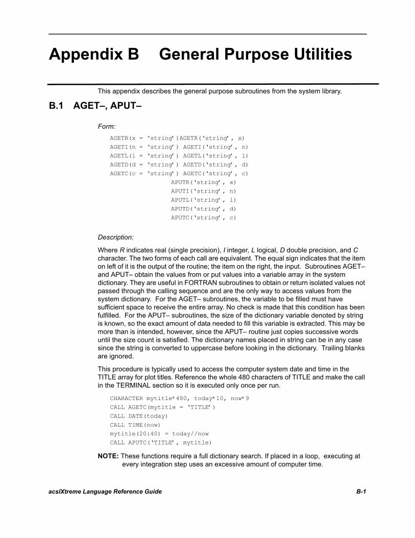
Appendix B General Purpose Utilities
This appendix describes the general purpose subroutines from the system library.
B.1 AGET–, APUT–
Form: AGETR(x = ‘string’)AGETR(‘string’, x)
AGETI(n = ‘string’) AGETI(‘string’, n)
AGETL(l = ‘string’) AGETL(‘string’, l)AGETD(d = ‘string’) AGETD(‘string’, d)
AGETC(c = ‘string’) AGETC(‘string’, c)
APUTR(‘string’, x)APUTI(‘string’, n)
APUTL(‘string’, l)
APUTD(‘string’, d)APUTC(‘string’, c)
Description:
Where R indicates real (single precision), I integer, L logical, D double precision, and C character. The two forms of each call are equivalent. The equal sign indicates that the item on left of it is the output of the routine; the item on the right, the input. Subroutines AGET– and APUT– obtain the values from or put values into a variable array in the system dictionary. They are useful in FORTRAN subroutines to obtain or return isolated values not passed through the calling sequence and are the only way to access values from the system dictionary. For the AGET– subroutines, the variable to be filled must have sufficient space to receive the entire array. No check is made that this condition has been fulfilled. For the APUT– subroutines, the size of the dictionary variable denoted by string is known, so the exact amount of data needed to fill this variable is extracted. This may be more than is intended, however, since the APUT– routine just copies successive words until the size count is satisfied. The dictionary names placed in string can be in any case since the string is converted to uppercase before looking in the dictionary. Trailing blanks are ignored.
This procedure is typically used to access the computer system date and time in the TITLE array for plot titles. Reference the whole 480 characters of TITLE and make the call in the TERMINAL section so it is executed only once per run.
CHARACTER mytitle*480, today*10, now*9CALL AGETC(mytitle = ‘TITLE’)
CALL DATE(today)
CALL TIME(now)mytitle(20:40) = today//now
CALL APUTC(‘TITLE’, mytitle)
NOTE: These functions require a full dictionary search. If placed in a loop, executing at every integration step uses an excessive amount of computer time.
acslXtreme Language Reference Guide B-1

B.2 DEBUG
Form: CALL DEBUG
Description:
A call to this routine produces a debug dump of all variables, excluding arrays greater than MALPRN (maximum array limit for print), on the print (PRN) unit. If HVDPRN (high volume display) is set TRUE, the dump also appears on the display (DIS) unit. The simplest way to get debug dumps is to set NDBUG to a positive integer at runtime so that a debug list is produced at the end of every DERIVATIVE, DISCRETE, and Jacobian evaluation; for example:
ACSL> SET NDBUG=20
ACSL> START
While useful as a checkout tool, with large programs this approach can result in an overwhelming amount of output. A more restricted selection of dumps can be obtained by using the ACTION command (see Chapter 5) or by including a call to DEBUG at the end of the DERIVATIVE or DISCRETE sections as follows:
IF(logical condition) CALL DEBUG
NOTE: Sorted sections of a program are not always translated in the order given. Reviewing the resulting FORTRAN listing will show the order of execution and the placement of the DEBUG call.
Including the following call in the DYNAMIC section produces the dump at every communication interval and is synonymous with OUTPUT /ALL:
CALL DEBUG
Calling DEBUG from the TERMINAL section gives all final values plus initial conditions, a useful set of data. Putting the call on a logical switch as follows allows you to suppress the listing when you don’t want it, such as during interactive runs.
LOGICAL dumpCONSTANT dump = .TRUE.
IF(dump) CALL DEBUG
B.3 DISSTR
Form: CHARACTER buffer*nnCONSTANT buffer = ‘ ‘
WRITE(buffer, label) a
CALL DISSTR(buffer)label: FORMAT(format)
Description:
In window environments (Microsoft Windows, X windows, etc) it is not possible to use Fortran WRITE and PRINT statements to write to screen, so the DISSTR (display string)
B-2 acslXtreme Language Reference Guide

utility is provided. Three of the examples (ACRFTS, ARESTG, and TESTER) under ACSL for Windows use the utility.
DISSTR writes to both the runtime window and the log file.
To use DISSTR, an internal file is declared as a character buffer with enough space to write a message (*80 for an 80-column line, for example). The information is written to the buffer in a WRITE statement, with the buffer name where a logical unit would normally be. A Fortran FORMAT statement follows the usual rules, except for a restriction on using a slash (/) for a line feed because it overflows the buffer; generate blanks in the output with further calls to DISSTR. (The format can be incorporated into the WRITE statement; see a Fortran programmer’s manual for details.) Finally, a call to DISSTR(buffer) prints the buffer.
For further information on writing to internal files, see a Fortran programmer’s manual or the ANSI standard reference book.
To illustrate the procedure, the following is an example is taken from the ARESTG model.
!--write the message to a buffer so that it can then be
! displayed as a string. It is given an initial value
! to prevent the message about used but not definedCHARACTER buffer*80; CONSTANT buffer = ‘ ‘
WRITE(buffer, 200) speed, ncase
CALL DISSTR(‘ ‘) ! write two blank linesCALL DISSTR(‘ ‘)
CALL DISSTR(buffer) ! write the message
CALL DISSTR(‘ ‘) ! write two blank linesCALL DISSTR(‘ ‘)
200: FORMAT(20x,’Aircraft speed - ‘,f6.2,’ Run no. ‘,i3)
B.4 INITD
Form: CALL INITD
Description:
A call to INITD clears the event list. This is useful for parametric runs which loop from TERMINAL to INITIAL and contain DISCRETE sections. If the event list is not cleared before looping back, multiple loops add events to the event list and produce erroneous multiple executions of events.
The event list cannot be cleared automatically by acslXtreme at the end of a run in case the user next commands a CONTINUE. CONTINUE skips over the INITIAL section and expects to continue with everything unchanged. The automatic initialization by acslXtreme in the INITIAL section takes place before the INITIAL section user code in order to allow the use of SCHEDULE within the INITIAL section. The event list is thus cleared automatically when the INITIAL section is executed in response to the START command, but not when a program loops back from the TERMINAL section. A call to INITD handles this loop situation. For an example using this utility, see the program in Appendix C of the User Guide on Temperature Distribution Along a Radiating Fin.
acslXtreme Language Reference Guide B-3

B.5 INTEG
Description:
The INTEG subroutine can be used to incorporate a user-written routine to provide flexibility in trying new and improved integration algorithms. Setting IALG=7 transfers control to the INTEG routine at the beginning of every integration step. Familiarity with the ACSL runtime routines ZZNITS, ZZNITA, ZZINTG, ZZRKIN, and INTEGZ(NST) is essential to write an effective INTEG routine.
B.6 LISTD
Form: CALL LISTD(unit)
Description:
The list dictionary call provides a listing of the user dictionary and current variable values along with any explanation of the variables supplied on the named file. Used mainly for reports, it requires preparing a dictionary file with variable names and definitions. The argument unit is an integer constant or a variable defining a FORTRAN file unit number containing the definitions. The file should be configured as follows:
column 1-9 variable name, left justified column 10 optional continuation indicator in sequence 0, 1, 2, 3, etc.
column 11-80definition
Because column 10 is reserved for continuation characters, only names up to nine characters long can be handled by the current version of LISTD. Invocation of the call is in the INITIAL or TERMINAL section, usually on a switch as follows:
LOGICAL list
INTEGER unitCONSTANT list = .FALSE. , unit = 11
IF(list) CALL LISTD(unit)
At the START runtime command, the dictionary is read from unit file (11 in the example). In Windows, the Open browser appears.
The dictionary is terminated by a blank name field or an end-of file. When a definition must be continued beyond column eighty, a non-blank character in column ten results in the name field being ignored and just the continued definition being listed out. Repeat the name on each continuation line, numbering the lines 0, 1, 2, 3, etc. in column ten. Now a standard sort on columns one through ten produces an alphabetical order with the continuation lines in their correct places. Note that zero is used in the first line of a continuation sequence and acts just like a blank. The reason for using a zero is that in some computer systems blanks collate after numbers rather than before.
ACSL issues a message if a variable name in the dictionary file is not found (if a name is misspelled, for instance). Duplicate names also result in an error message. If the name is in the program but the value is undefined, asterisks appear in the value column. For arrays, the type and size of the array is given, rather than all the values in the array; for example, REAL(3).
B-4 acslXtreme Language Reference Guide

The dictionary listing appears on the high volume print unit PRN, the log file of the runtime session. If system symbol HVDPRN has been set TRUE, the listing also appears on the screen during an interactive session. The log file can be read and/or accessed with an editor to update the dictionary file for subsequent runs.
See the Missile Airframe example in Appendix C of the User Guide for an example using LISTD.
B.7 RSTART
Form: CALL RSTART(blockname, newstep)
Description:
Where blockname refers to a DERIVATIVE section (which must have been given a name) and newstep is an integration step size. A call to the RSTART routine restarts the step size and history of the variable step, variable order integration algorithms (IALG = 1 or 2). It has no effect on the fixed-step Runge-Kutta algorithms (IALG = 3, 4, or 5). It cannot be used with the Runge-Kutta-Fehlberg algorithms (IALG = 8 or 9). The call is usually used within a DISCRETE section that may be changing conditions discontinuously, thus invalidating the history data used by the integration routine in the continuous section.
The use of RSTART is not required since the variable step algorithms control the step to satisfy an error criterion, but RSTART can help reduce the amount of work done by the integration routine if a drastic change in step size is known to be necessary.
B.8 SETI, SETR
Form: CALL SETI(iv, ia, n)
CALL SETR(rv, ra, n)
Description:
Where the value of expression iv or rv is set into n locations of array ia or ra; n is an integer variable, i indicates type INTEGER, and r indicates floating point (REAL or DOUBLEPRECISION depending on the mode chosen at translation). The SET– subroutines are provided primarily to initialize arrays and set all elements to a given value. A complete array may be set, for example:
CALL SETR(k*a, array, iset)
or only a portion of an array:
CALL SETR(0.0, arr(5), 3)
in which case zeros are placed in the fifth, sixth, and seventh elements of array ARR. No check is made to see whether these elements actually exist.
acslXtreme Language Reference Guide B-5

B.9 WEM
Form: CALL WEM(‘character string’)
Description:
The WEM (write error message) utility write a message to both the print (PRN) and display (DIS) logical units.
B.10 XFERBR, XFERBI
Form: CALL XFERBR(y = x, n)CALL XFERBI(j = i, n)
Description:
Where x and y are floating point arrays of the same length, i and j are integer arrays of the same length, and n is an integer specifying the number of elements in the arrays. If n is a variable, it must be declared as an INTEGER. The XFERB– (transfer block) subroutines move arrays from one place to another without requiring DO loops. The n elements in array x are moved into array y. No check is made to see whether these elements actually exist. XFERBR is single or double precision, depending on its arguments. XFERB– might be used, for example, to transfer the three elements VM(1), VM(2), and VM(3) into the first three elements of the array RMD as follows:
CALL XFERBR(rmd = vm, 3)
B-6 acslXtreme Language Reference Guide

Appendix C acslXtreme System Symbols
C.1 IntroductionMany system constants can be set at runtime with the SET command to control printing and integration.
NOTE: The name must not have been used in the program code for a symbol to be accessed at runtime.
Each system symbol is listed below along with its type, default value, and description. The value set by the user must agree with the symbol in type; i.e., integer into integer, logical into logical, floating point or integer into floating point, and character into character.
The first three characters of the symbols describe the action. The last three characters describe the symbol group as follows:
- ITG integration control
The symbols are listed below by group.
C.2 Integration control
CIOITG
(INTEGER, ...) Current integration order of variable order integration routines (IALG = 1 or 2). This variable is calculated by the program and may be OUTPUT or PREPAREd so that the integration order can be monitored.
CJVITG
(LOGICAL, TRUE) Check Jacobian validity. A report is issued if the Jacobian is considered invalid.
CSSITG
(REAL, ...) Current step size taken by the integration routine. This variable is calculated by the program and may be OUTPUT or PREPAREd so that the actual integration step size can be monitored.
DPSITG
(LOGICAL, TRUE) Double precision states; i.e., when TRUE, the state variables are accumulated in double precision. The default is FALSE on 64 bit computers.
ECSITG
(LOGICAL, FALSE) Errors based on current state. Determines whether the allowed errors for the variable step integration routines are based on current state values TRUE or on the largest values of the states so far.
acslXtreme Language Reference Guide C-1

MXOITG
(INTEGER, 6) Maximum order of the integration algorithm may be specified between 1 and 6 when using the variable order, variable step integration routines (IALG = 1 or 2).
NRWITG
(LOGICAL, FALSE) No rewind. When this flag is TRUE, the RRR (raw run record) data file (i.e., the file containing the values logged for all the variables on the PREPARE list) is not rewound at the beginning of a START or CONTIN command (the normal procedure). This feature enables accumulation of data from sequential runs, which then can be printed and/or plotted at the end of all the runs.
TJNITG
(REAL, 0.2) Threshold for flagging Jacobian nonlinearities; 1.0 effectively turns it off. In order to see the results, CJVITG should be TRUE.
TSMITG
(LOGICAL, FALSE) Two-sided matrix evaluation for the stiff integration algorithm (IALG = 2) to evaluate the linearized state transition matrix. If the state equation is dx ¤ dt = F(x), then the two sided matrix is obtained from F(x+dx) and F(x-dx); the single sided matrix from F(x) and F(x-dx). While the two sided matrix is more accurate than the single sided, it requires twice as long to evaluate the complete matrix.
WEDITG
(LOGICAL, TRUE) Write event description when using the SCHEDULE operator for state events. This data can be suppressed by setting WEDITG to FALSE..
WESITG
(LOGICAL, TRUE) Write error summary for variable order, variable step integration routines (IALG = 1 or 2). All the states, along with the count of the number of times each state controlled the integration step size, are listed at the end the run. This data may be suppressed by setting WESITG to FALSE.
WNDITG
(LOGICAL, FALSE) Write normal data during integration; i.e., basic information about the integration process (slightly different for each integration algorithm) so that it can be followed.
WXDITG
(LOGICAL, FALSE) Write extra data during integration; i.e., Jacobian matrix, which is not written out when WNDITG is TRUE because it can be very high volume depending on the number of state variables.
C-2 acslXtreme Language Reference Guide

4-1
Symbols! 4-1, A-3- 1-1& 4-1, A-3) 4-92= 4-2
AABS 4-5ACOS 4-5acslXtreme language 1-2acslXtreme operator
integration 1-3acslXtreme statements 1-3action characters A-5Adams-Moulton 4-10add
line 1-2text 1-2
AGET– B-1AINT 4-6algebraic loop 3-5ALGORITHM 4-6
Adams-Moulton 4-10Array with multiple sections 4-7DASSL 4-11Determining appropriate step size 4-
13Efficiency and accuracy 4-14Error summary 4-13Fixed step algorithms 4-8Gear’s stiff 4-10MINT 4-12NSTP 4-13Recommended integration
control 4-7Runge-Kutta procedure 4-9Variable step algorithms 4-10
ampersand 4-1ampersand (&) A-3Angles A-4ANINT 4-14
APUT– B-1arithmetic
assignment statement 4-15, 4-16operator position 2-5operators 2-5
arithmetic operators 1-3array
name conflict 4-3order 2-3
ASIN 4-15assignment statement
arithmetic 4-15, 4-16character 4-16
Assignment statementsArithmetic 4-15Character 4-16Logical 4-16
ATAN 4-16ATAN2 4-17
BBCKLSH 4-17block diagrams 1-1BOUND 4-18
CCALL 4-18case sensitive A-4CHARACTER 4-19
variable 2-3character
assignment statement 4-16CHARACTER (See TYPE)character constant 2-3characters
special 4-1CINTERVAL 4-19
Adjusting step size to CINT 4-20Bound on integration step 4-21Calculating CINT 4-20Changing default name 4-21Double precision 4-20
CINTERVAL operatordefinition 1-5
CIOITG C-1
acslXtreme Language Reference Manual 1
2
CJVITG C-1CMPXPL 4-22code
comment 1-6continuation 1-6seperator 1-6
colon 4-1comma A-3COMMENT 4-23comment 4-1Comment (!) 4-23comment, code 1-6Comments (!) A-3concatenation operator 5-2CONSTANT 2-1, 3-5, 4-23
recomputation 4-1variables defined 4-1
constant 2-1character 2-3floating point 2-2logical 2-2
Continuation 4-25continuation 4-1Continuation (&) 4-25CONTINUE 4-26
attach statement label 2-4CONTINUE statement 2-5control
transfer 3-4conventions 1-2
Command lines 1-2keyboard keys 1-2Menu items 1-2Variables 1-2
copy/pastetext 1-2
COS 4-26CSL A-2CSL code window 1-1CSSITG C-1
DDASSL 4-11DBLE 4-27DBLINT 4-27
DEAD 4-29DEBUG B-2debugging 4-2
LOGD 4-2default names 1-6DELAY 4-29delete 1-1DELSC 4-31DELVC 4-32DERIVATIVE 4-33DERIVATIVE section 3-3
state variables 4-3DERIVATIVE statement
definition 1-5Derivatives A-5DERIVT 4-34
Jacobian calculation 4-35sorting 4-35
differential algebraic system solver (See DASSL)
differential operators 1-3DIM 4-35DIMENSION 4-36directive statements
Macros 5-5DISCRETE 4-37DISCRETE section 3-3, 5-3DISSTR B-2DO 4-38DOUBLE PRECISION 4-39Double precision C-1DOUBLE PRECISION (see TYPE)DOUBLEPRECISION 4-5double-precision 1-2DPSITG C-1drag-and drop 1-2DYNAMIC 4-39, A-4DYNAMIC section 3-3
multiple sections 3-5
EECSITG C-1END 4-40END Statement
definition 1-5
acslXtreme Language Reference Manual

END statement A-4equal sign 4-2
use in PROCEDURE 4-2Equations
sorting 1-3error control 1-2Errors C-1ERRTAG 4-40exclamation point 4-1EXP 4-41expansion
macro 2-4explicit structure 3-1expression
arithmetic operators 2-5definition 2-5
FFCNSW 4-41floating point 2-2Fortran statements
conventional 1-1free-form input function generation 1-
2
GGAUSI 4-42GAUSS 4-43Gear’s stiff 4-10general purpose subroutines B-1GO TO 4-43Greek letters A-5
HHARM 4-44HISTORY 4-45
IIALG 4-6IF 4-46IF-THEN-ELSE 4-46IMPLC 4-48implicit structure 3-1IMPVC 4-51INCLUDE 4-52
INITD B-3INITIAL 4-53INITIAL section 3-3, 5-3
multiple sections 3-5INT 4-54INTEG 1-3, 1-4, 4-55, B-4
scalar integration 1-3INTEGER 4-57
variable 2-3integer
constant 2-1promotion 2-2
INTEGER (See TYPE)Integration 1-3
routine 3-3integration algorithm C-2Integration Control
CIOITG C-1CJVITG C-1CSSITG C-1DPSITG C-1ECSITG C-1MXOITG C-2NRWITG C-2TJNITG C-2TSMITG C-2WEDITG C-2WESITG C-2WNDITG C-2WXDITG C-2
Integration control C-1integration operator 1-3integration operators 1-3INTERVAL 4-57INTVC 4-58
vector integration 1-3
JJacobian
check validity C-1flagging nonlinearities C-2
Kkeywords
program structure A-2
acslXtreme Language Reference Manual 3
4
Llabel 2-4
CONTINUE statements 2-4reserved 2-4statement labels and macro
expansion 2-4syntax 2-4
labels A-4language
acslXtreme statements 1-3arithmetic operators 1-3MACRO capability 1-3standard functions 1-3
language syntax 2-1LEDLAG 4-59library functions 1-3LIMINT 4-60LISTD B-4Lists
CONSTANT statements A-3Dimension A-3type A-3
LOG 4-62LOG10 4-62LOGD
debugging 4-2LOGICAL 4-63
variable 2-3logical constant 2-2loop
algebraic 3-5LSW 4-63
MMACRO 4-64
expansion 2-4macro
block definition 5-3standalone 5-2
MACRO ASSIGN 5-6MACRO capability 1-3MACRO CONTINUE 5-7MACRO DECREMENT 5-7MACRO DIVIDE 5-8MACRO EXIT 5-8
MACRO GO TO 5-8MACRO IF 5-8, 5-12MACRO INCREMENT 5-9MACRO MULTIPLY 5-9MACRO PRINT 5-9MACRO REDEFINE 5-9MACRO RELABEL 5-9MACRO STANDVAL 5-10Macros 5-1
Arithmetic macro directives 5-7defined 5-1Dimensions 5-12directive statements 5-5Dot product 5-11examples 5-11Expansion 5-12features 5-1REDEFINE 5-12Sampler 5-11Second type 5-12
mathematical convention A-2mathematical equations 1-1matrix
two-sided evaluation C-2MAX 4-64MAXTERVAL 4-64MERROR 4-66MIN 4-67MININTERVAL (See MAXTERVAL)MINT 4-12MINTERVAL 4-64, 4-68MOD 1-3, 4-68modeling
nonlinear differential equations 1-1time-dependent equations 1-1transfer functions 1-1
modifiers A-5modulus 1-3MXOITG C-2
Nname
default 1-6Name length A-5names
acslXtreme Language Reference Manual

reserved 1-6naming system A-4nesting sections 3-5NINT 4-68NRWITG C-2NSTEPS 4-69NSTP 4-13number
floating point 2-2
Oobject characters A-5operator
ACSL 4-3simulation model 4-2standalone 4-4
Operators A-2logical operators A-2
operatorsarithmetic 1-3backlash 1-2dead zone 1-2logical 1-3precision of 4-5quantization 1-2relational 1-3variable time delay 1-2
OU 4-70output
conversion to non-standard units A-4
PPARAMETER 4-72Parentheses A-3plotting
flexibility 1-2precision
forcing 4-5precision of operators 4-5PROCEDURAL 4-73, A-4
blockstate variables 4-3
PROGRAM 4-75program
job processing 1-2program layout
Readability A-1program sorting 3-4Program structure
keywords A-2program structure A-2programming
general structure A-2Golden Rule A-1
programming restriction A-2programming style A-1promotion of integers 2-2PTR 4-75PULSE 4-76
QQNTZR 1-3, 4-77quantization 1-3question mark 4-1
RRAMP 4-77REAL 4-78
LOGICAL 4-106variable 2-3
REALPL 4-78redundant state variable 1-4reserved names 1-6
alphanumeric character 1-6digit 1-6System variable default names 1-6
RESET 4-79rewind C-2RRR C-2RSTART B-5RSW 4-63, 4-80RSW (See LSW)RTP 4-80Runge-Kutta procedure 4-9Runge-Kutta-Fehlberg 4-11runtime
setting system constants C-1
acslXtreme Language Reference Manual 5
6
SSAVE 4-81SCALE 4-81SCHEDULE 4-82
State Event Mechanization 4-88State Event Specification 4-88Time Event 4-88Time Event Specification 4-86
sectionDERIVATIVE 3-3DISCRETE 3-3, 5-3DYNAMIC 3-3, 5-3INITIAL 3-3, 5-3nesting 3-5TERMINAL 5-3
select text 1-2semicolon 4-1separator 4-1, 4-92Separator ( 4-92SET command C-1SETI B-5SETR B-5SIGN 4-92Simulation
applications 1-1biomedical systems 1-1chemical process
representation 1-1control system design 1-1fluid flow 1-1heat transfer analysis 1-1microprocessor controllers 1-
1missile and aircraft
simulation 1-1power plant dynamics 1-1vehicle handling 1-1
compiled simulation 1-2physical systems 1-1
Simulation Control Commands 1-2simulation model
operator 4-2SIN 4-93single-precision 1-2
SORT 4-93special characters 4-1SQRT 1-3, 4-93square root 1-3standalone macro 5-2standard functions 1-3state variable 3-4state variables
operators 4-3statements 4-1STEP 4-95step size C-1STOP flag 3-3structure
explicit 3-1implicit 3-1
subroutinesgeneral purpose B-1
subscripted variable 2-3symbol
concatenation 5-2syntactical elements 4-1syntax, acslXtreme language 2-1
TTABLE 4-96TAN 4-100TEMPLATE.CSL A-1Templates A-1TERMINAL 3-4, 4-100TERMINAL section 5-3
multiple sections 3-5TERMT 4-101TERMT statement
definition 1-5TJNITG C-2TRAN 4-102transfer control 3-4translator 4-1TRANZ 4-104TSMITG C-2TYPE
CHARACTER 4-106DIMENSTION 4-106DOUBLEPRECISION 4-106
acslXtreme Language Reference Manual

INTEGER 4-106REAL 4-106
Type 4-106
Uunderscore 2-3UNIF 1-3, 4-108UNIFI 4-42, 4-108uniform random number 1-3uniformity A-1Units A-4
English A-4SI A-4
VVARIABLE 4-108variable
array order 2-3CHARACTER 2-3INTEGER 2-3LOGICAL 2-3REAL 2-3redundant state 1-4state 3-4subscripted 2-3types 2-3
variables 4-1
WWEDITG C-2WEM B-6WESITG C-2wild card 4-1window
CSL code 1-1WNDITG C-2WXDITG C-2
XXERROR 4-66, 4-108XERROR (See MERROR)XFERBI B-6XFERBR B-6
acslXtreme Language Reference Manual 7