©

or3©

o

©

DEPARTMENT OF MECHANICAL ENGINEERING & MECHANICS

COLLEGE OF ENGINEERING & TECHNOLOGY

OLD DOMINION UNIVERSITY

NORFOLK, VIRGINIA 23529

AN ANALYTICAL APPROACH TO GRID SENSITIVITY ANALYSIS

FOR NACA FOVR-DIGIT WING SECTIONSI

J _ z

By

I. Sadrehaghighi, Graduate Research Assistant

p

_j _ , ". v I . ,

! / • ,

and

S.N. Tiwari, Principal Investigator

Progress Report

For the period ended December 1991

Prepared forNational Aeronautics and Space Administration

Langley Research CenterHampton, Virginia 23665

Under

Cooperative Agreement NCC1-68Dr. Robert E. Smith Jr., Technical Monitor

ACD-Computer Applications Branch

(N_SA-C_-19OZ_I) AN ANALYTICAL APPROACH TOL;P,[3 _CNSITIV|IY ANALYSIS F_R NAC_i:_?Uq-!_I_IT WIN_ SECTIONS _ro:jress Ref_ort t 1Jan. - "__ uec.j 19____91(.91ci Dominion Univ.)

N92-25175

Uncl dsG3/O? 0089,,05

April 1992

https://ntrs.nasa.gov/search.jsp?R=19920015932 2018-06-11T00:43:55+00:00Z

DEPARTMENT OF MECHANICAL ENGINEERING & MECHANICS

COLLEGE OF ENGINEERING & TECHNOLOGY

OLD DOMINION UNIVERSITY

NORFOLK, VIRGINIA 23529

AN ANALYTICAL APPROACH TO GRID SENSITIVITY ANALYSIS

FOR NACA FOUR-DIGIT WING SECTIONS

By

I. Sadrehaghighi, Graduate Research Assistant

and

S.N. Tiwari, Principal Investigator

Progress Report

For the period ended December 1991

Prepared for

National Aeronautics and Space Administration

Langley Research Center

Hampton, Virginia 23665

Under

Cooperative Agreement NCC1-68Dr. Robert E. Smith Jr., Technical Monitor

ACD-Computer Applications Branch

Submitted by theOld Dominion University Research FoundationP.O. Box 6369

Norfolk, Virginia 23508-0369

April 1992

FOREWORD

This is the progress report on the research project " Numerical Solutions of Three-

Dimensional Navier-Stokes Equations for Closed-Bluff Bodies". Within the guidelines

of the project, special attention was directed toward research activities in the area

of "Grid Sensitivity in Airplane Design." The period of performance of this specific

research was .January 1, 1991 through December al, 1991. This work was supported

by the NASA Langley Research Center through Cooperate Agreement NCC1-68.

The cooperate agreement was monitored by Dr. Robert E. Smith Jr. of Analvsis and

Computation Division (Computer Applications Branch), NASA Langley Research

Center," Mail Stop 125.

lU

F_T.CF.._i_IG PP,G_ BL.._NII_ i"4,OT F];....MED

ABSTRACT

An Analytical Approach To Grid Sensitivity

Analysis For NACA Four-Digit Wing Sections

Ideen Sadrehaghighi"

Surendra N. Tiwari t

Sensitivity analysis in Computational Fluid Dynamics with emphasis on gricls and

surface parameterization is described. An interactive algebraic grid-generation tech-

nique is employed to generate C-type grids around NACA four-digit wing sections.

An analytical procedure is developed for calculating grid sensitivity with respect to

design parameters of a wing section. A comparison of the sensitivity with that ob-

tained using a finite-difference approach is made. Grid sensitivity with respect to

grid parameters, such as grid-stretching coefficients, are also investigated. Using the

resultant grid sensitivity, aerodynamic sensitivity is obtained using the compressible

two-dimensional thin-layer Navier-Stokes equations.

"Graduate Research Assistantt Eminent Professor

iv

TABLE OF CONTENTS

FOREWORD ................................................................. iii

ABSTRACT .................................................................. iv

TABLE OF CONTENTS ...................................................... v

NOMENCLATURE .......................................................... vii

Chapter

T T

1. INTRODUCTION .......................................................... 1

'2. ALGEBRAIC GRID GENERATION ........................................ :3

2.1 Basic Formulation ...................................................... 3

2.2 Grid Algorithm ......................................................... 4

3. PROBLEM STATEMENT AND METHOD OF SOLUTION ................. 7

3.1 Theoretical Formulation ................................................. 7

3.2 Surface Parameterization ................................................ 8

3.3 grid sensitivity .......................................................... 8

4. WING-SECTION EXAMPLE . ............................................. 10

4.1 wing-Section Parameterization ......................................... 10

4.2 Grid Sensitivity With Respect To Control Parameters .................. 13

4.2 Flow Sensitivity With Respect To Control Parameters .................. 15

5. RESULTS AND DISCUSSIONS ............................................ 17

5.1 NACA 0012 Airfoil Test Case .......................................... 17

5.1.1 Grid Sensitivity .................................................. 17

5.1.2Flow Sensitivity .................................................. 18

5.9 NACA 8512Airfoil Test Case .......................................... 19

5.2.1Grid Sensitivity .................................................. 19

5.2.2Flow Sensitivity

6. CONCLUSION ............................................................ 32

REFERENCES ............................................................... 34

APPENDICES:

A. FORTRAN LISTING OF GRID GENERATION ALGORITHM ......... 37

B. FORTRAN LISTING FOR NACA FOUR-DIGIT SURFACE

GENERATION ........................................................... 42

C. FORTRAN LISTING OF NACA FOUR-DIGIT GRID SENSITIVITY ... 50

vi

NOMENCLATURE

**

X"

R

P

XD

U

V

X, y, z

Xl, Yl

T

3

t

KI, K2

T

M

C

Cp

CD

= vector of field variables

= vector of physical coordinates

= steady-state residual

= vector of control parameters

= vector of design parameters

= horizontal interpolant

= normal interpolant

= physical coordinates

= airfoil surface coordinates

= surface grid distribution function

= far-field boundary grid distribution function

= grid stretching function

= surface orthogonality function

= far-field boundary' orthogonality function

= orthogonality parameters

= stretching parameter

= maximum thickness parameter

= maximum camber parameter

= camber location parameter

= pressure coefcient

= drag coefficient

vii

CL

CI

Cx, Cr

YT

P,

U, U_ _U

p

Moo

P_

Re_

3 _

0

Ot

Ti

= lift coefficient

= skin friction coefficient

= force coefficients in z and y directions

= camber line coordinates

= section thickness distribution

= surface pressure

= velocity components in z , y and z directions

= density

= energy per unit volume

= free-stream Mach number

= free-stream density

= free-stream velocity

= free-stream Reynolds number

= computational coordinates

= horizontal blending function

= normal blending function

= surface slope

= angle of attack

= surface skin friction

.°.

Vlll

1. INTRODUCTION

Over the past several years, Computational Fluid Dynamics (CFD) has

rapidly evolved. This has been the result of the immense advances in computational

algorithms [1] and the development of supercomputers. These innovations have had a

major impact on obtaining numerical flow simulations about complex geometri.es. On

current supercomputers, viscous-compressible flow simulations about aircraft config-

uration can require several hours per steady-state solution [2]. Such large amounts

of computational time are acceptable for proof-of-concept studies and selective anal-

ysis, but they are not acceptable for optimization and design. With advent of the

next generation of parallel supercomputers [3], airplane design and optimization using

nonlinear CFD (Euler and Navier-Stokes equations) should become routine. For an

individual component, such as a wing, it is now reasonable to consider design and

optimization in conjunction with nonlinear CFD [4].

An essential element in design and optimization is acquiring the sensitivity

of functions of CFD solutions with respect to control parameters. For aerodynamic

surfaces, the control parameters specify the shapes of the surfaces. This affects the

surface grid and the field grid which, in turn, affects the flow- field solution. There are

two basic components in obtaining aerodynamic sensitivity. They are: (1) obtaining

the sensitivity of the governing equations with respect to the state variables; and (2)

obtaining the sensitivity of the grid with respect to the defining parameters. The

sensitivity of the state variables with respect to the defining parameters are described

by a linear-algebraic relation [,5]. This study concentrates on the grid sensitivity and

parameterization of aerodynamic surfaces.

The simplest method for calculating grid sensitivity is basedupon finite-

differenceapproximation. In this approach, a designparameter is perturbed from

the nominal value, a new grid is obtained, and the differencebetween the new and

the old grid is used to obtain the grid sensitivity derivatives. This direct, or brute

force technique, has the disadvantagesof being computationally intensive. It is the

objectiveof the analytical approachto avoidthe time consumingand costly numerical

differentiation. In addition, the analytic derivativesareexact insteadof approximate.

Taylor et al. [6] set the stagefor the developmentof the technique usedin

this study. For a steady-statesolution of the Euler or Navier-Stokesequations, the

sensitivity of a function of the solution with respect to the control parameters is to

be found. The problem includes the determination of sensitivity of the grid with

respectto control parameters. For grid generation,algebraic transfinite interpolation

[7] is ideally suited for the study of parameterization. Parametersare sub-grouped

according to their purposes (grid spacingcontrol and surface shapecontrol). The

objective is to cast the surfaceparameterization in terms of designparametersrather

than geometric variables. Geometric parameterization has only local control and

consequentlyrequireslarge numberof parametersto definea grid. A specializedap-

plication of transfinite interpolation [8] is cast in terms of designparametersfor a

classof wing sectionsand wings. The grid sensitivity of this system is discussed.

2. ALGEBRAIC GRID GENERATION

2.1 Basic Formulation

Structured algebraic grid generation techniques can be thought of as trans-

formations from a rectangular computational domain to an arbitrarily-shaped physi-

cal domain [7]. The transformations are governed by the vector of control parameters

P. That is,

where

x(4,_,¢,p)={ x(4,_,¢,P)u(_,_,¢,P) :(_,_,¢,P)}r

0<_1, O<q_l, and O<C_I.

(_1)

A discrete subset of the vector-valued function X(_i, rb, ¢'k, P ) - X { z y z },rs. k - X*

is a structured grid for _i = _"_,i-1r5 = .Z.=.LM_I,¢'k = _,k-1_'--'-7,where i = 1,2,3... , L, j =

1,2,3,-.-,M and k= 1,2,3,.-.,N.

The dominant algebraic approach for grid generation is the Transfinite In-

terpolation scheme. The general methodology was first described by Gordon [9] , and

there have been numerous variations applied to particular problems. The methodol-

ogy can be presented as recursive formulas composed of univariate interpolations [10]

or as the Boolean sum of univariate interpolations [7]. Here, we follow the Boolean

sum representation but; for brevity, we restrict the process to two dimensions and

omit some of the details that can be found in Ref. [7]. Also, to be consistent with

the example considered below, the parameterization is restricted to functions and first

3

4

derivativesat the boundaries(_ = 0, 1) and (r/ = 0, 1) and control in the interpolation

functions. The transformation is

X(_,r/,P)=UoV=U+V-UV (2.2)

where

and

2 1 )0nX(O' _' PT) (2.,3)

I=1 n=O

, omx(¢,w, pS)V = _ _ 3y(r/,P_) ) (2.4)

J=, m =0 Orlm

The term UV (not expanded here) is the tenser product of the two univariate interpo-

lations. The boundary, curves and their derivatives _(o"X((t'n'PT)0n_and a"x(_,,a.P_0,,, ) I, J =

1,2 m,n = 0,1) are blended into the interior of the physical domain by the in-

terpolation functions ai(_,P_0) and /32(7, P_). The boundary grid, the derivatives

at the boundary grid and the spacing between points are governed by the param-

eters {P5 , TPI} • The interpolation functions are controlled With the parameters

P0} • The entire set of control parameters can be thought of as a vector

{P ova P5PT} v.

2.2 Grid Algorithm

An interactive univariate version of Eq.(2.2) using only the normal interpolant V is

developed. This, known as Hcf'mite Cubic Interpolation, matches both the function

and its first derivative at two boundaries. An analytical approximation of the physical

coordinates for a class of wing sections can be expressed as

Oxl(r,P_)x = x_(r, P_)Z°(t, P_))+ R(r)_(t, P_))

Ot

+ x:(s,P_)3°(t,P_)+ S(s)OX_(_tP_)3_(t,P_) (2.s)

where

and

y = y1(r,P_)'d°(t,P;) + R(r)0y,(r, P_Ot )3_(t, P;)

+ y2(s, _ ,o Oy2(s,P_)fl_(t,p_)P2),d2(t, Pg) + S(s) Ot

9(t, P_)= 2t 3- 3t 2 + 1,

_(t, pg} = t_ - 2t_+ t,

,3°(t,pg)= _2t _ + at_,

, t n t3/32(t, Po) = - t

O<t<l.

(2.6)

Five functions r = f_(sx), s = k(_), R(r) = K,J'a(_), S(s) = K_f4(_) and

t = fs(r]) and their implied defining parameters control the grid spacing on the bound-

aries and the interior grid. Functions r and s define the grid spacing for lower and

upper boundaries respectively, while R(r) and S(s) specify the magnitude of orthog-

onality along those boundaries. The parameter t defines the grid distribution for the

connecting curves between the two boundary. The quantities Ka and Ks are param-

eters that scale the magnitude of the orthogonality at the boundaries. Increasing Kt

and K_ extends the orthogonality of the grid into the interior domain. Excessively

large values of K1 and K2 can also cause the grid lines to intersect themselves, which

is not a desirable phenomena.

A discrete uniform distribution of the computational coordinate, can be

mapped into an arbitrary distribution of the physical coordinate, using the specified

control function. The essence of mapping, is that the abscissa corresponds to the per-

centage of grid points and the ordinate corresponds to a particular control function

which, in turn, relates to the geometric definition of the physical domain. The control

function, can be either a specified analytical function, or for more general purposes,

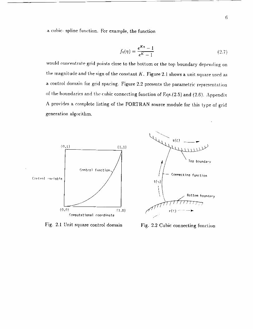
a cubic- spline function. For example, the function

e t<" - 1

£(7)- _ 1 (2.7)

would concentrate grid points close to the bottom or the top boundary depending on

the magnitude and the sign of the constant K. Figure 2.1 shows a unit square used as

a control domain for grid spacing. Figure 2.2 presents the parametric representation

of the boundaries and the cubic connecting function of gqs.(2.5) and (2.6). Appendix

A provides a complete listing of the FORTRAN source module for this type of grid

generation algorithm.

(0 I) (l.l)

Co.trol ,'ariableControl funct

(o,o) (1.o)Computat{onal coordinate

Fig. 2.1 Unit square control domain

/ Top boundary

I _ Connectino function

t(.)

oundary

/

Fig. 2.2 Cubic connecting function

3. PROBLEM STATEMENT AND METHOD

OF SOLUTION

3.1 Theoretical Formulation

let Q be a solution of the Euler or Navier-Stokes equations on the domain X and

Q* be a discrete solution on the grid X* where

and

{ / {Q" = p pu pv pw pc ,,j,k X*= x y z i,j,k

OQ

o--t- = R(Q'(X'),X') = 0. (3.2)

Here, R(Q*(X'), X') is the residual of a steady-state solution as t _ de. Let P be a

vector of parameters that controls the grid X" such that X" = X((i, r/j, q'k, P) where

(, r] and (,"are computational coordinates [7]. The numerical sensitivity of a function

F(Q(X)) with respect to the control parameters is

FP(Q'(X')) = { OF(_pX')) } = { OF(Q'(X')) } { OQ*(X*) }OQ"0P " (3.3)

The fundamental sensitivity equation containing {_} and described by Taylor

et al. [6] is

OR(Q'(X'), X')OQ'(X')[OR(Q'(X'), X')] OX" "_

It is important to notice that Eq.(3.4) is a set of linear, algebraic equations

[0R(Q'iX'),X')] and [°R(Q;(xX.')'X') ] are well understood [6]. The, and the matrices L 0q'(x') l

7

quantitiy {_} is the solution to Eq.(3.4) given the sensitivity of the grid with

respectto the parameters. Therefore, the grid sensitivity problem is describedby

0X" _ GridSensitivity}

3.2 Surface Parameterization

In Eq.(2.2), the parameterization is on the boundaries and in the interpo-

lation functions. The most general parameterization of the boundaries would be to

specify every grid point X_j (i.e., each boundary grid point is a parameter). This

conceivably could be desirable for the boundaries corresponding to an airplane surface

to allow a design procedure to have the greatest possible flexibility. This, however,

is impractical from a computational point of view. A compromise is to specify the

knots of a spline function or the control polygon for a B4zier function. Even with this

compromise, it could require hundreds of parameters for a wing. Here we propose a

quasi-analytical parameterization in terms of design variables. For instance, a class of

wing sections is specified by two camber-line parameters and a thickness distribution

parameter; a wing is specified by several wing sections; and the wing surface is inter-

polated from the sections. In this manner, an airplane component can be specified

by tens of parameters instead of hundreds or ,housands of parameters. The disad-

vantage is that a great deal of generality is not available, but the generality is a moot

point if computational capacity cannot accommodate it. For design and optimization

with CFD, at the present time, it is advocated here to use a small number of design

parameters for boundary definition.

3.3 Grid Sensitivity

As it is stated in the introduction, the simplest way to obtain grid sensitivity

with respect to the parameterization is to vary the parameters and finite difference the

results. This is computationally expensive compared to analytically differentiating

Eq.(2.2). Therefore, we propose the latter. Grid sensitivity can be used for grid

adaptation, or it can be used for boundary design. For adaptation, the grid sensitivity

with respect to those parameters that control the grid spacing and the shape of the

field grid _way from fixed boundaries are desired. The sensitivity is used to improve

some grid-quality function of the solution. For design and optimization the sensitivity

of the grid with respect to the parameters that define the shape of a boundary is

desired. The sensitivity is used to improve a design function of the solution.

4. WING-SECTION EXAMPLE

4.1 Wing-Section Parameterization

Much research has been devoted to the development and representation of

wing sections. The NACA four-digit wing sections are examined for grid-generation

parameterization. Families of wing sections are described by combining a mean line

and a thickness distribution. The resultant expressions possess the necessary features

that suit the problem, mainly the concise description of a wing section in terms of

several design parameters. Reference 11 provides the general equations which define

a mean line and a thickness distribution about the mean line. The design param-

eters are: T - the maximum thickness, M - the maximum ordinate of the mean

line or camber, and C = chordwise position of maximum ordinate. The numbering

system for NACA four-digit wing-section is based on the geometry of the section.

The first and second integers represent M and C respectively, while the third and

fourth integers represent T. Symmetrical sections are designated by zeros for the

first two integers, as in the case of NACA 0012 wing-section. Figure 4.1 provides a

schematic of the section definition. The (-coordinate is first mapped into the chord

line :_ = _'(r) = 5:(f1(_)) forward and then reversed to cover both the top and bottom

of the section. The mean line equation is

M 5:2Yc(_) = _-+(2C_ - ), +: _< C (4.1)

Yc(_) = M (1 - 2C + 2C_ - _:) _ > C. (4.2)(1 -C) 2 ' -

10

11

The section thickness is given by

T tFT(2) = 7--7,,(0.29691"2 - 0.1

O.2-

The section coordinates are

262 - 0.3516_ _ + 0.284323 - 0.101524). (4.3)

x,(r,P{)=2 y,(r,P{)=_)c(_)+gT(2. ). (4.4)

Figures 4.2 and 4.3 show sample grids for NACA 0012 and NACA 8512

section using this procedure. The orthogonality at the far-field boundary is ignored.

For solid boundary, the orthognality is obtained using the components of unit normal

vector at the surface

P_I ) _ T sinOOXl(r,

Ot (Oyl(r, Pi))Oy,(r,P{) _ +cosO O = tan-' \Oz,(,', P{)Ot

(4.5)

Figure 4.4 shows a wing-surface grid derived from three differently-specified

sections in the spanwise direction. The surface grid results from the distribution

function fl({), and interpolation of the design parameters for the three wing sections

in the spanwise direction. In addition to the three .!esign parameters for each wing

section, it is necessary to specify their relative chord lengths and positions. The

additional design parameters can be: leading edge sweep, trailing edge sweep, dihedral

angle, reference chord length, and section-span locations.

Leading edge

Thickness

"'_ Mean camber line

Fig. 4.1 Schematic of wing-section

Trailing

edge

12

i 1 ]I ]

n ' !

; i

l li_in

iI

Fig. 4.2 Example grid for NACA 0012 wing-section

L

' iE

"J!"-'-"

i

Fig. 4.3 Example grid for NACA 8512 wing-section

t:l

Fig. 4.4 Example wing surface grid (top view)

Appendix B provides the source module for generating the surface of NACA four-digit

wing-sections.

4.2 Grid Sensitivity With Respect To Control

Parameters

There are two types of control parameters involved in this analysis. First, there

are the design parameters (T, M, and C) which specify the shape of the primary

boundary and secondly, there are tile parameters that define the other boundaries

and the the spacing between grid points. Here we express, in part, the sensitivity of

tile grid with respect to the design parameter vector XD, and with k a stretchir_g

parameter in the interpolation functions related by fs(r/,k)). The grid sensitivity

with respect to design parameters at the outer boundary has been ignored. Also, due

to zero orthogona[ity at the outer boundary, a direct differentiation of Eqs.(2.5) and

(2.6) with respect to X D yields to

Ox Ox 0xl(r, P_)

OqXD OXl 0XD

Oz 0x'_(r, P_)+ (_)

0x'_ 0XD

14

Oy Oy 0y'l(r,P_) 0y 0yl(r,P_)- +

0X D Oy_ 0X D o9yl 0X D1.7)

where

XD = (T,M,C) 1.S)

o_ ov _ _o(t,p_) o_ os = n(_)_l(t,p_). 1.9)0xl - 0y, Txl = 0y--i,

The prime indicates differentiation with respect to t and can be substituded from

Eq.(4.5). Since x1(r, P_) is independent of design parameters XD, then

Oxl(r,e_) -0.0. (1.10)0XD

The x coordinate sensitivity, Eq.(4.6), can now be reduced to

Ox iO(g:sinO) (Oyl(r'PI) ) (1.11)0X D - R(r)3l(t,P_}, OqXD 0 = tan -1 \Oxl(r,P_) "

Using the relation

0--tart-lit =

0XD

the x coordinate sensitivity becomes

1 Ou

1 + u 2 0XD(1.12)

Ox 1 0 0yl(r, P_)0XD - _R(r)_q_(t'P'°)c°sO . (1.13)

(Om(r,P])) 20XDOxl(r, Pi)1 + oxl(r,P_)

The term ° ovl(.,Pi)0XD a.l(_,P_) can be evaluated by direct differentiation of Eq.(4.4). The y

coordinate sensitivity with respect to design papameters can be obtained using similar

procedure. Equation (4.7) can be modified to

Oy

OXD uA D

1 0 Oyl(r, P_I )

1+2 0X D 0Xl(r, p_)'

(1.14)

All terms at the right hand side of Eqs.(4.13 ) and (4.14) can be evaluated explicitly

due to analytical parameterization of the surface for this particular example. The

grid sensitivity with respect to the stretching parameter [¢ are

Ox Xl(r,p_)OO°(t,P_) Ot Oxl(r,P_)O_(t,P;) Ot0_: - Ot Of( + R(r) O_ Ot Of_

1.5

where

+ x2(r,p_)O3°(t' P_) OtOt Or`

+ S(s)Ox2(s'P_)O3_(t,P_) atat or, (4.1,5)

03°(t,P_) _ 6t 2 _ 6tOt

O3°(t' P_)) - -6t 2 + 6tOt

O3{(t,P_) _ 3t 2 _ 4t + 1Ot

03_(t,P_)) _ 3t 2 _ 1.Ot

An example of the stretching function is

t - el__ 1 (4.16)

at (e f_ - 1 )77e_ - (e_ - 1)e f_

Or`- (e_ - 1)_ (4.17)

Similar developments can be extended to other grid control parameters such

as the distribution of grid point around the wing section and magnitude of orthogo-

nality at the boundaries. Appendix C provides the source module for grid sensitivity

of NACA four-digit wing-sections with respect to design parameters.

4.3 Flow Sensitivity With Respect To Control

Parameters

The flow sensitivity coefficient {_} can now be evaluated using the

fundamental sensitivity equation, Eq.(3.4). The Jacobian matrices [OR(Q'(X').X')][ oQ.(X.) j

_nd[o"/q;g.'/x'l]_eobtained_in__n_mpli__ime_n_e_ionofthe_D_h_nlayer Navier-Stokes equations [10]. These equations are solved in their conservation

form using an upwind cell-centered finite-volume formulation. A detailed description

of the procedure is found in Refs. [12-17] and is not repeated here. A third-order

accurate upwind biased inviscid flux balance is used in both streamwise and normal

16

directions. The finite-volumeequivalentof second-orderaccuratecentral differencesis

usedfor viscousterms. For a typical designanalysisof an airfoil, the flow sensitivity

coefficient { c,q'(x')0p } provides far more information than needed. In most cases, the

sensitivity of aerodynamic forces on the surface, such as lift and drag coefficients,

are sought. For such analysis, only a small subset of the flow sensitivity coefficient

{ c_q'(X')aP } (i.e. surface properties)is needed since the lift and drag coefficients can

be expressed as

Cc = Cvcosa - Cxsina

CD = Cysin_ + Cxcosa

(4.18)

(4.19)

where a is the flow angle of atack. The quantities Cx and Cy are the total force

coefficents along a: and y directions respectively and can be expressed as

NE

CX -_ E Cp,(_ti+l - yi) -_- C],(Zi+l - £i) (4.20)i=1

NE

= - + - (4.:?:)i=1

where Cpi and Ca,, are pressure and skin friction coefficients respectively

Pi ri@' = 1,, r,2" Cf,- _ 2 (4.22)

and NE represents total number of bondary cells along airfoil surface. The terms Pi

and ri are pressure and shear stress associated with boundary cell i and the quantity

1 2_p_oU_ is known as dynamic pressure of the free stream . Finally, the drag and lift

sensi'tivity coefficients with respect to XD are obtained by differentiating Eqs.(4.18)

and (4.19) as

OC L OCy (_C X- cosa sina (4.23)

0XD 0X D 0XD

OCL c)Cv OCxsins. (4.24)

69XD -- OX DcOsct 0X D

5. RESULTS AND DISCUSSION

5.1 NACA 0012 Airfoil Test Case

5.1.1 Grid Sensitivity

The first test case considered is the NACA 0012 symmetrical airfoil. The

previously obtained grid, as shown in Fig. 4.2, is considered for grid sensitivity anal-

ysis. The grid sensitivity with respect to the vector of design parameters XD, are

obtained using Eqs. (4.13) and (4.14). The maximum thickness T is the only design

parameter for this case.

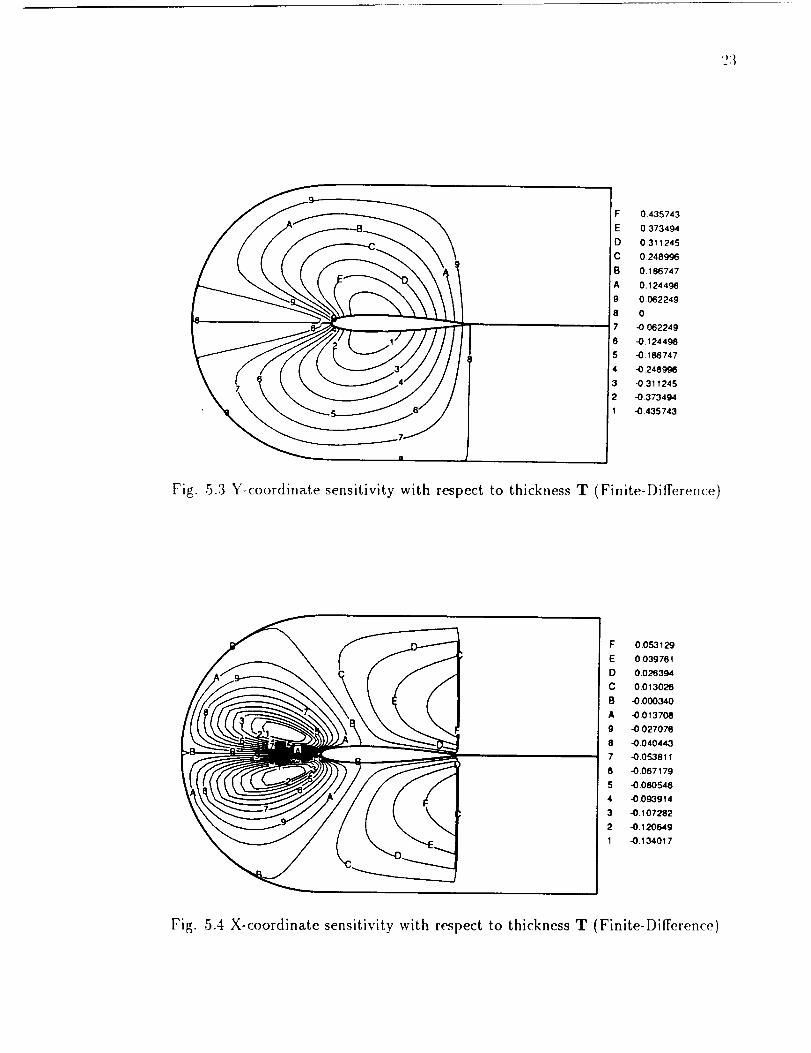
Figure 5.1 shows the contour levels of the y-coordinate sensitivity with re-

spect to the thickness parameter, T. The highest contour levels are, understandably,

located in the vicinity of the chordwise location for the maximum thickness of the

wing section. For a NACA four-digit wing section, this is positioned about 0.3 of

the chord length from the leading edge [11]. The positive and negative contour levels

corresponding to the upper and lower surfaces are the direct consequence of Eq.(4.4)

and the second term on the right hand side of Eq.(4.7). The sensitivity levels decrease

when approaching the far-field boundary due to diminishing effects of the interpola-

tion function/31°(t, P_)). The first term on the right hand side of Eq.(4.7) is responsible

for the sensitivity effects due to orthogonality on the surface, and it is directly pro-

portional to the magnitude of the orthogonality vector K1. The wake region is not

sufficiently affected by any of the design parameters, and no major sensitivity gradi-

ent should be expected there.

17

1S

Figure 5.2 demonstrates the contour levels of the x-coordinate sensitivity

with respect to thickness parameter, T. An interesting observation can be made here

regarding the contour levels adjacent to the surface. Unlike the y-coordinate sensitiv-

ity, the x-coordinate sensitivity has its lowest value on the surface. This can be traced

back to Eq.(4.4), which indicates that x-coordinates on the surface are basically inde-

pendent of the design parameters. The only remaining factor is the second term on

the right hand side of Eq.{4.6) which is the effect of the surface orthogonality vector.

There are some negative pockets of contour levels on the forward section and some

corresponding positive pockets on the rear section. The dividing line between these

pockets i.s located near the location of the maximum thickness (i.e., 0.3 of chord from

leading edge). A simple conclusion from Fig. 5.2 is that by increasing the thickness

parameter, T points on the forward section will move to the left, while at the same

time, points at rear section will move to the right.

For comparison purposes, the grid sensitivity for this case is obtained using

the finite difference approach. The design parameter(i.e. T for this case) are per-

turbed, one at a time, and a new grid is obtained using Eqs.(2.5) and (2.6). The

sensitivity is then computed using a central difference approximation and the results

are presented in Figs. 5.3 and 5.4. A side by side comparison of both results indicates

good agreement between the two approaches.

5.1.2 Flow Sensitivity

The second phase of the problem is obtaining the flow sensitivity coefficients

using the previously obtained grid sensitivity coefficients. In order to achieve this,

according to Eq. (3.4), a converged flow field solution about a fixed design point

should be obtained. The computation is performed on a C-type grid composed of 141

points in the streamwise direction and 31 points in the normal direction. It is appar-

ent that such a coarse grid is inadequate for capturing the full physics of the viscous

19

flow over an airfoil. Therefore, it shouldbe understood that the main objective here

is not to producea highly accurateflow field solution rather than to demonstratethe

feasibility of the approach.

A free stream Mach number of M_ = 0.8, Reynolds number Re_ = 106 ,

and angle of attack a = 0 ° is used. Figures 5.5 and 5.6 demonstrate the pressure and

Mach number contours of the converged solution. Figure 5.7 shows the surface pres-

sure coefficient Cp, where the lift and drag coefficient for this particular example are

CL = 1.53x10 -8, CD = 4.82x10 -2. The sensitivities of the aerodynamic forces, such

as drag and lift coefficients with respect to thickness parameter T, are obtained uti-

lizing Eqs.(4.18-4.24). The corresponding results are presented in Table 5.1. Again.

for comparison purposes, a finite difference approximation has been implemented to

validate the results. A nominal perturbation of 10 .3 for design parameter T has been

chosen and the corresponding results are included in Table 5.1. The good agreement

between the two sets of numbers verifies the accuracy of the approach.

Another important goal of using sensitivity analysis, apart from optimiza-

tion, is the approximation analysis. An approximate version of Eq.(3.4) can be used

to predict the steady-state solution changes which occur in response to geometric

shape changes. Such a method is valid as long as the changes in geometric shape

(i.e., design parameter) are small. Figure 5.8 shows the non-linear relation between

drag coefficient and thickness parameter T verifying the above argument.

5.2 NACA 8512 Airfoil Test Case

5.2.1 Grid Sensitivity

The second test case considered is the NACA 8512 cambered airfoil. Again,

the previously obtained grid, as shown in Fig. 4.3, is considered for grid sensitivity

analysis. Figures 5.9 and 5.10 show the y and x-coordinate sensitivity with respect

to parameter T respectively. Their characteristics are similar to the previous sym-

2O

metrical airfoil case;hence,detailed description of their behavior is omitted here.

Figure 5.11 representsthe y-coordinate sensitivity with respect to camber,

M. It appearsthat the highestsensitivity contour levelsare located at the chordwise

location of camber,C (i.e., 0.5of chord length). The contour levelsdecreasetoward

the far-field boundary, again as a consequenceof interpolation function. However,

unlike Fig. 5.9 here they possesspositive valueson both upper and lower surfaces.

Consequently,an increasein camber,M, shifts all the points upward. Again, mini-

mum activity can bedetectedin the wakeregion. Figure 5.12showsthe x-coordinate

sensitivity contourswith respectto camber,M. Here,asin Fig. 5.10, the sensitivities

are minimum on the surfaceof the wing-section. There is a small gradient on the

forward section,but by far, the strongestgradient is in the rearward section due to

orthogonality effects.

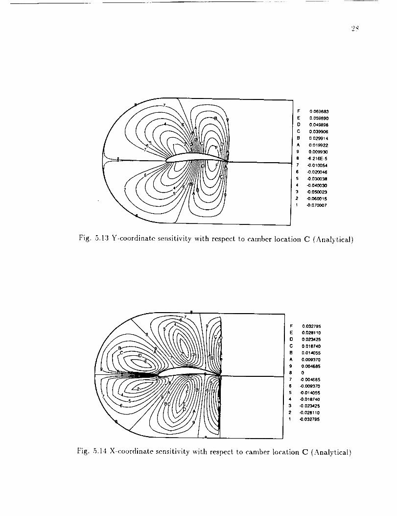
Figure 5.13 illustrates the y-coordinate sensitivity with respect to camber

location, C. A dividing line betweenpositive and negative contour levelsappears

near the chordwiseposition of the camber. Like previouscases,there is nosignificant

activity in the wakeregion. The result indicatesthat a positivechangeof C will cause

the movementof points downwardon the forward section,while at the sametime, the

points on the rear sectionwill respondby moving upward. Figure 5.14 illustrates the

x-coordinate sensitivity with respect to camberlocation C. The two major features

are attributed to chordwiselocation of the camber and the orthogonality effectson

the tail section. It is interesting to notice that the sensitivity level for camberlocation

is considerablylessthan the other two designparameters.

Similar developmentscanbeextendedto other grid control parameterssuch

as the distribution of grid point around the wing section and magnitude of orthogo-

nality at the boundaries. For example, the grid sensitivity with respect to stretching

parameterk, using Eqs.(4.15-4.17),is obtained and the resultsare presentedon Figs.

5.15and 5.16.

21

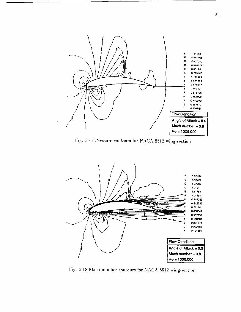
5.2.2 Flow Sensitivity

Using free stream conditions of M_ = 0.8 , Re_ = 10 6, and a = 0 °, a

converged flow field solution is obtained. As in previous case, a C-type grid of 141x31

is used. Figures 5.17 and 5.18 illustrate the pressure and Mach number contours.

Figure 5.19 shows the surface pressure coefficient Cv, where lift and drag coefficients

are CL = 0.106, and CD = 0.0738. The aerodynamic sensitivity coefficients with

respect to vector of design parameters XD, are obtained and presented in Table 5.2.

A comparison with finite difference validates the accuracy of the approach.

,) .)

F 0435752

E 0.373501

D 0.311251

C 0.249001

B 0.186751

A 01245

9 0062250

8 -1.117E-8

7 -0.062250

6 -0.1245

5 -0.186751

4 -0.249001

3 -0.311251

2 -0.373501

1 -0.435752

Fig. 5.1 Y-coordinate sensitivity with respect to thickness T (Analytical)

_ B

C DF 0.053905

E 0.040511

D 0.027116

C 0.013722

B 0000328

A -0.013065

9 -0.026459

8 -0.039853

7 -0.053248

6 -0 066642

5 -0.080036

4 -0093430

3 -0.106825

2 -0.120219

I -0.133613

Fig. 5.2 X-coordinate sensitivity with respect to thickness T (Analytical)

F 0,435743

E 0.373494

O 0.311245

C 0248996

B 0.186747

A 0,124498

9 0.062249

8 0

7 4) ,062249

6 -0,124498

5 -0.186747

4 -0.248996

3 -0,311245

2 -0.373494

1 -0,435743

Fig. 5.3 Y-coordinate sensitivity with respect to thickness T (Finite-Difference)

F 0,053129

E 0.039761

D 0.026394

C 0.013026

B -0.000340

A -0.013708

9 -0.027076

8 -0.04044,3

7 -0.053811

.-0.067179

5 -0.080546

4 -0.093914

3 -0.107282

2 -0.120649

1 -0,134017

Fig. 5.4 X-coordinate sensitivity with respect to thickness T (Finite-Difference)

'21

/

1

F 1.06457

E 1.02346

O 0.982351

C 0.941241

B 0.900131

A 0.859021

9 0.817911

8 0.776801

7 0,735691

0,694582

5 0.6,_3472

4 0,812362

3 0,571252

2 0,530142

1 0.489032

FIow Condition: I "Angle of Attack = 0.0 J

Mach Number = 0.8 /

Re = 1000,000 /

Fig. 5.5 Pressure contours for NACA 0012 wing-section

F 1.15471

E 1.07773

D 1.00075

C 0 923772

B 0.846791

A 0,76981

9 0.892829

8 0,615848

7 0.538867

6 0,461886

5 0 3849O5

4 0 307924

3 0230943

2 0.153962

1 0.076981

I Flow Condition: l

Angle of Attack = 0.0

Mach Number = 0.8

Re = 1000,000

Fig. 5.6 Mach number contours for NACA 0012 wing-section

,:,+)

l'_ L_ su_Ac_

:ii-vsl_

I;ig. 5.7 S,rrn('e l)r¢,,ssm-e coemcient for NACA 0012 wing-section

0 0;'%

(Symrneltlcal NACA Alrtoil)

";0 7S lO+O I_.S 15.0 17.SM_¢, Thlckr_ee (% Chord|

I"i_,_. :,.,_ I)r,_p: rovllh:ieut Vs Maxi,mm 'l'hicl(ness

'l:,l,h, S.I I,ifl. ;,_.1 I)rag sensiLiviLies wiLh respeeL to design paramet, er T

.... ; - ,)

I)<'_;g. l';,ra_tf.+'l,('r_

.\+, +--'I'h hl_ t.'+<:;._

DirecL Approach FiniLe Differe, ce

82( n a,_n OX n 8,_ n-2.68×10 -_ 0.709 -4.?5x10 -_ O.TOT

26

F 0.435743

E 0.373494

O 0,311245

C 0.248996

B 0.186747

A 0124498

9 0,06224g

8 0

7 -0062249

8 -0,124498

5 -0.186747

4 -0.248996

3 -0.311245

2 -0.373494

1 -0.435743

Fig. 5.9 Y-coordinate sensitivity with respect to thickness T (Analytical)

F 0.038276

E 0,008127

D -0.022021

C -0.052170

B -0.08232

A -0,112469

9 -0.142618

$ -0.1 72767

7 -0.202916

8 -0.233065

5 -0.283214

4 -0.293364

3 -0,323513

2 -0.353662

1 -0,383811

Fig. 5.10 X-coordinate sensitivity with respect to thickness T (Analytical)

27

F 0.937473

E 0.874975

D 0.812477

C 0.749979

B 068748

A 0624982

9 0.562484

8 0.499986

7 0.437488

6 0.374989

5 0.312491

4 0.249993

3 0.187495

2 0.124996

1 0.062498

Fig. 5.11 Y-coordinate sensitivity with respect to camber M (Analytical)

F 0.197091

E 0.168935

0 0.140779

C 0.112623

B 0.084467

A 0.056311

9 0.028155

8 0

7 -0 _028155

6 -0.056311

5 -0.084467

4 -0.112623

3 -0.140779

2 -0.168935

1 -0.197091

Fig. 5.12 X-coordinate sensitivity with respect to camber M (Analytical)

2_

F 0.069883

E 005989O

D O.0498g8

C 0039906

B 0029914

A 0019922

9 0.009930

8 -6.216E-5

7 -0.010054

6 -0.020046

5 -0030038

4 -0.040030

3 -0.050023

2 -0.06001S

1 -0.070007

Fig. 5.13 Y-coordinate sensitivity with respect to camber location C (Analytical)

7

O

C

B

A

9

8

7

6

5

4

3

2

1

F 0032795

E 0028110

0,023425

0.018740

0,014055

OOO9370

0.004685

0

-0004685

-0OO9370

-0.014055

-0.018740

-0.023425

-0.028110

-.0,032795

Fig. 5.14 X-coordinate sensitivity with respect to camber location C (Analytical)

,)i..,)

F 0.344228

E 0.204034

D 0.24384

C 0.193646

B 0.143452

A 0093258

g 0,043064

8 -0007129

7 -0,057323

6 -0.107517

5 -0.157711

4 -0.207g05

3 -0258099

2 -0,308293

1 -0 358487

Fig. 5.15 Y-coordinate sensitivity with respect to stretching parameter

F 0.041860

E 0.010620

D -0,020619

C -0,05185g

B °O.083100

A -0,11434

g -0.14558

8 -0.176821

7 -0208061

6 -0.23g301

5 -0270641

4 -0.301781

3 -0.333021

2 -0.364262

I -0.395502

Fig. 5.16 X-coordinate sensitivity with respect to stretching parameter

/

F I 042£,6

E 0 9099,68

O 0937272

C 0 8_,A 578

B 0 83_88

A 0 779185

g 0 72_41_9

8 0673793

7 0 62t097

0 5_8401

5 0 515705

4 0 4 c_3009

3 0410313

2 0357617

1 0.304921

Flow Condilion: 1

Angle of Attack = 0.0

Mach number = 0.8

Re = 1000,000

Fig. 5.17 Pressure contours for NACA 8512 wing-sect, ion

F 1 52397

E I 42228

O _ 320_

C 12191

B 1.11751

1 01591

0 914323

8 0.812732

7 0.71114

0609549

'5 0507957

4 0 406366

0 304774

2 0 203183

I 0 101591

Flow Condition:

I Angle of Attack = 0.0Mach number = 0.8

Re = 1000,000

Fig. 5.18 Math nlmd)er contours for NACA 8512 wi.g-section

3l

o _

J

o,_

o0

-O 5

• 1.0

Fig. 5.l!1 Surface pressure coefficient for NACA 8512 wing-section

'l'al,le 5.2 l,ift and [)rag sensitivities with respect to vector of design

parameters XD

NA_CA 5x2l)csigu l'arameters

,k'v = Thickness

Xo = (3amber

,kt) = Camber location

Direct Approachoc_Eo.

OXn OXn

-1.058 0.410

7.840 0.322

_8.34x10 "3 -,l.31x10 -3

Finite Difference

8X _ ,, OX n

- 1.058 0.410

7.838 0.322

-8.5x10 "_ -4.3xX0 -s

6. CONCLUSION

The objective of this study has been to demonstrate an approach for ob-

taining grid sensitivity which can be used in aerodynamic design and optimization.

It is shown that grid sensitivity is an essential ingredient in the calculation of aero-

dynamic sensitivity. The main supposition is that a grid is defined algebraically in

terms of parameters and computational coordinates. Therefore, coordinates of the

grid and derivatives of the coordinates with respect to the parameters (grid sensi-

tivity) are computed directly as functions of the parameters and uniformly-discrete

values of the computational coordinates. A subset of the parameters defines the shape

of the grid boundaries which corresponds to the aerodynamic surfaces of interest. It

is recommended that the aerodynamic surfaces be parameterized in terms of design

parameters which have global control. As compared to a geometric parameteriza-

tion, this drastically reduces the number of parameters. However, it limits the design

flexibility. In addition to the aerodynamic surface parameters, the sensitivity with

respect to parameters that define other boundaries, such as the far-field boundary or

the spacing of grid points, is available for analysis or grid adaptation.

The algebraic grid-generation scheme and NACA wing sections presented

here are intended to demonstrate the elements involved in obtaining grid sensitivity

from an algebraic grid generation process. It is evident that each grid generation

formulation would require considerable analytical differentiation. This implies that

a symbolic manipulator, which directly produces computer code for derivative eval-

uation, should be considered. Also, there are trade-offs between analytical differen-

32

33

tiation and finite-differencedifferentiation. It may be feasible to obtain someof the

derivatives bv finite differences.

It is implied that airplane surfacesshould be parameterizedin terms of de-

sign variables. This is not simple or feasiblefor geometrically-complexairplanes in

advancedstagesof design. However,designparameterization is feasibleduring con-

ceptional and preliminary design. The parameterization, which is the development

of analytical formulas for part or all of a surface is critical for satisfactory results.

It is always possible to create a geometric parameterization of a surface (collection

of points or derivatives that define surface patches), but geometric parameterizations

have very local sensitivities and a complete aerodynamic surface can require a large

number of parameters for its definition.

As a compromise between totally analytic parameterization of surfaces and

geometric parameterization, a hybrid approach is advocated. In a hybrid approach,

certain sections or skeletal parts of a surface are specified analytically and interpo-

lation formulas are used for the remainder of the surface. This is employed for the

wing example described herein.

REFRENCES

1. Elbanna, H., and Carlson, L., "Determination of Aerodynamic Sensitivity Co-

efficients in the Transonic and Supersonic Regimes," AIAA Paper 89-0.532. Jan-

uary 1989.

° Huband, G. W., Shang, J. S., and Aftosmis, M. J., "Numerical Simulation of an

F-16A at Angle of Attack," Journal of Aircraft, Vol. 27, pp. 886-892, October

1990.

3. Corcoran, E., "Calculating Reality," Scientific American, Vol. 23, pp. 101-109,

January 1990.

4. Smith, R. E., and Sadrehaghighi, I., "Grid Sensitivity in Airplane Design,"

Proceedings of the fourth International Syposium on Computational Fluid -

Dynamics, Vol. 1, September 9-12, 1991, Davis, California, pp. 1071-1076.

, Sobieszczanski-Sobieski, J. "The Case for Aerodynamic Sensitivity Analysis,"

Paper presented to NASA/VPI SSY Symposium on Sensitivity Analysis in En-

gineering, September 25-26, 1986.

6. Taylor, A. C., III, Hou, G. W., and Korivi, V. M., "Sensitivity Analysis Applied

to the Euler Equations : A Feasibility Study with Emphasis on Variation of

Geometric Shape," AIAA Paper 91-0173, January 1991.

7. Eiseman, P. R., and Smith, R. E., "Applications of Algebric Grid Generation

, Applications of Mesh Generation to Complex 3-D Configurations," AGARD-

CP-464, pp. 4-1-12, 1989.

34

35

8. Smith, R. E., and Wiese,M. R., "Interactive Algebraic Grid-Generation Tech-

nique," NASA TechnicalPaper2533, March 1986.

9. Gordon, W. N., and Hall, C. A., "Construction of Curvilinear Coordinate Sys-

tems and Application to MeshGeneration," Journal of Numerical Methods for

Engineers, Vol. 7, pp 461-477, May 1973.

10. Smith, R. E., and Eriksson, L. E., "Algebraic Grid Generation," Comp. Meth.

Appl. Mech. Eng., Vol. 64, pp 285-300 , 1987.

i 1. Abbott, I. H., and Von Doenhoff, A. E.,Theory of Wing Sections, Dover, New'fork..

1959.

12. Taylor, A. C., III, Hou, G. W., and Korivi, V. M., " Sensitivity Analysis, and

Design Optimization For Internal and External Viscous Flows," AIAA Paper

91-3083, September 1991.

13. Taylor, A. C., III, Hou, G. W., and Korivi, V. M., " An Efficient Method For

Estimating Steady-State Numerical Solutions to the Euler Equations," AIAA

Paper 91-1680.

14. Taylor, A. C., III, Hou, G. W., and Korivi, V. M., " A Methodology for Deter-

mining Aerodynamic Sensitivity Derivatives With Respect to Variation of Geo-

metric Shape," Proceedings of the AIAA/ASME/ASCE/AHS/ASC 32nd Struc

15.

tures, Structural Dynamics, and Materials Conference, April 8-10, Baltimore,

MD, AIAA Paper 91-1101, April 1991.

Baysal, O., and Eleshaky, M. E., "Aerodynamic Sensitivity Analysis Methods

for the Compressible Euler Equations," Recent Advances in Computational Fluid-

Dynamics, (ed. O. Baysal), ASME-FED Vol. 103, 11th Winter Annual Meeting,

November, 1990, pp. 191-202.

36

16. Baysal,O., and Eleshaky,M. E., "Aerodynamic DesignOptimization UsingSen-

sitivity Analysis and Computational Fluid Dynamics," AIAA Paper 91-0471,

January 1991.

17. Korivi, V. M., " Sensitivity Analysis Applied to the Euler Equations," M.S.

Thesis , Old Dominion University, Norfolk, VA, June 1991.

18. Yates, E. C.,dr., "Aerodynamic Sensitivities from Subsonic,Sonic,and Super-

sonicUnsteady,NonplanarLifting-SurfaceTheory,"NASA TM-100502, Septem-

ber 1987.

APPENDIX A

FORTRAN LISTING FOR GRID GENERATION

ALGORITHM • HERMITE

37

File: b Dinted Tue Jan 01 00:00:00 1980

SUBROUTINE HERMITE1 (XS, YS, NI, NJ, ALFA, XGRD, YGRD, PROBID, DOBATCH)

PARAMETER (NGRID=3)

$ INCLUDE tbggl, inc

$ INCLUDE tbgg5, inc

DIMENSION XS (NGDIM, *), YS (NGDIM, *), T (NGDIM), XGRD (NGDIM, NGDIM)

1 ,YGRD (NGDIM, NGDIM), ALFA (NGDIM), S1 (NGDIM, NGDIM)

2 ,XLEFT (NGDIM), YLEFT (NGDIM), XRIGHT (NGDIM), YRIGHT (NGDIM)

3 ,RI (NGDIM), RO (NGDIM), R (NGDIM), S (NGDIM), SK (NGDIM)

4 ,X (NGDIM), Y (NGDIM), XVIEW (NGDIM, NGDIM), YVIEW (NGDIM, NGDIM)

COMMON/PQ/PS (MGDIM), QS (MGDIM), tS (MGDIM, MGDIM)

COMMON/DXYDETA/DXBDETA (NGDIM), DYBDETA (NGDIM)

COMMON/JAYS/Jl, J2, J3

common/design/cm, p, th, rr, wlength, chord

CHARACTER PROBID* (*), PR(4) *80

SAVE RO, XLEFT, YLEFT, XRIGHT, YRIGHT

LOGICAL REDRAW, DONE, REDIST, DOBATCH, FIRST

C

C

C

C ......

35

C Does basic grid calculations, draws grid, and provides for user

C modifications in interactive loop.

C-

C

C

c

299

C

C

99

C

C

C

C

C

C

C

C

C

REDIST = .FALSE.

REDIST = .TRUE.

DONE = .FALSE.

DONE = .TRUE.

Magnitude Of Orthogonality Vector

WRITE (*, *)

WRITE (*, *) ' Magnitude

READ(*,*) SKB

DO 299 I = 1 ,

SK(I) = SKBCONT INUE

NI

of Normal Derivatives ?'

CONT INUE

Uses

Distribution For Stretching Variable T

Linear Distribution For Initial Trial

Disribution For Final Trial

IF(REDIST.AND.(.NOT.DONE)) THEN

DONE = .TRUE.

IF (DOBATCH) THEN

CALL BATCH (NJ, RO, 5)

ELSE

CALL DISTXI (NJ, RO, 5)

ENDIF

DO I00 I = 1 , NI

and Arc-length

File: b Printed Tue Jan O1 00:00:00 198

C

199

C

C

C

C

101

C

C

C

C

102

C

100

C

C

C

C

C

C

C

201

C

DO 199 J = 1 , NGDIM

X(J) = XGRD(I,J)

Y(J) = YGRD(I,J)

CONTINUE

CALL ARC (X, Y, R, NGDIM, RMAX)

DO i01 J = 1 , NGDIM

RI(J) = R(J) / RMAX

IF (RI (NGDIM) .NE. I. 0) RI (NGDIM) =i. 0

CONTINUE

CALL INTERPO (RI, T, NGDIM, RO, S, NJ)

DO 102 J = 1 , NJ

SI(I,J) = S(J)

tS(I,J) = SI(I,J)

CONT INUE

CONT INUE

ELSEIF ((.NOT.REDIST) .AND. (.NOT.DONE)) THEN

REDIST = .TRUE.

DO 201 I = 1 , NI

DO 201 J = 1 , NGDIM

T (J) = FLOAT (J-l)/FLOAT (NGDIM-I)

SI(I,J) = T(J)

tS(I,J) = SI(I,J)

CONT INUE

C ......... Base Line Distribution

C

ELSEIF (REDIST.AND.DONE) THEN

107

C

C

IF (DOBATCH) THEN

CALL BATCH (NJ, RO, 5)

ELSE

CALL DISTXI (NJ, RO, 5)

ENDIF

DO 107 I = 1 , NI

DO 107 J = 1 , NJ

SI(I,J) = RO(J)

tS(I,J) = SI(I,J)

CONT INUE

ENDIF

IF (MGDIM.NE.NGDIM) THEN

WRITE (*, *)' >>>> tbggl.inc & tbgg5.inc Should Have the

:39

File: b Printed Tue Jan O1 00:00:00 198

1

STOP

ENDIF

Same Dimension'

C

C

Hermite Interpolation Function (Eq.3 of manual)

C

C

C

C

C

C

C

C

C

C

C

C

C

C

C

C

C

C

C

C

C

C

SKT = 0.0

DO 240 I=I,NI

XB = XS(I,1)

YB = YS(I,1)

XT = XS(I,2)

YT = YS(I,2)

........... Orthogonality For Foil

IF (I .GE. 1 .AND. I .LE. J2) THEN

DXDETA = - SIN(ALFA(I) )

DYDETA = + COS(ALFA(I) )

ELSEIF (I .GT .J2 .AND. I .LE .NI} THEN

DXDETA = + SIN(ALFA(1))

DYDETA = - COS (ALFA(I))

ENDIF

DXBDETA (I) =DXDETA

DYBDETA (I ) =DYDETA

IF(I.EQ.J2-4)SK(I} = SKB * 0.85

IFiI.EQ.J2-3)SK(I) = SKB * 0.75

IF(I.EQ.J2-2)SK(I) = SKB * 0.65

IF(I.EQ.J2-1)SK(I) = SKB * 0.55

IF(I.EQ.J2) SK(1) = SKB * 0.45

IF(I.EQ.J2+I)SK(I) = SKB * 0.55

IF(I.EQ.J2+2)SK(I) = SKB * 0.65

IF(I.EQ.J2+3)SK(I) = SKB * 0.75

IF(I.EQ.J2+4)SK(I) = SKB * 0.85

PS(1) = SK(I)

QS (I) = SKT

IF ( .NOT .DONE) THEN

N=NGD 114

ELSE

N=NJ

ENDIF

DO 240 J = I , N

4O

File: b PrintedTue Jan 01 00:00:00 198

C

C

C

240

C

C

C

CALL BLENDF(SI(I,J),FI,F2,F3,F4)

XGRD(I,J) = XB*FI + XT*F2 + PS(I) * DXDETA * F3

YGRD(I,J) = YB*FI + YT*F2 + PS(I) * DYDETA * F3

CONT INUE

IF ( .NOT .DONE) GOTO 99

RETURN

END

4 !

APPENDIX B

FORTRAN LISTING FOR NACA FOUR-DIGIT SURE-kCE

GENERATION" NACA

42

File: a Printed Tue Jan 01 130:00:00 1980 Page: 1

,)SUBROUTINE NACA (I S, XS, YS, NL I, ALFA, DOBATCH, CHEAT )

$INCLUDE tbggl, inc

PARAMETER (NGRID=3)

DIMENSION XS (NGDIM, 4) ,YS (NGDIM, 4) ,NLI (4), ALFA(NGDIM)

1 ,X0U (NGDIM), YOU (NGDIM), XOL (NGDIM), YOL (NGDIM)

2 ,YC (NGDIM), XCI (NGDIM), YT (NGDIM), DYTDXCI (NGDIM)

3 ,DYCDXCI (NGDIM), ETA (NGDIM)

DIMENSION XI (NGDIM), YI (NGDIM), XO (NGDIM), YO (NGDIM), RI (NGDIM)

1 ,RO (NGDIM), ROBAR (NGDIM), X (NGDIM), XX (NGDIM)

2 ,XU (NGDIM), YU (NGDIM), XL (NGDIM), YL (NGDIM), XDIST (NGDIM)

COMMON /A/A1, A2, A3, A4, A5

COMMON /DESIGN/CM, P, TH, R, WLENGTH, CHORD

COMMON/TANGENT/ALFAU (NGDIM), ALFAL (NGDIM), DYUDX (NGDIM), DYLDX (NGDIM), NFOIL

COMMON/OLD/XUS (NGDIM), YUS (NGDIM), XLS (NGDIM), YLS (NGDIM)

LOGICAL REDIST (3), DOBATCH, CHEAT

DATA PI,CK/3.14159,7./

>>>> NACA FOUR DIGIT AIRFOIL SECTION <<<<

COMPUTES AN AIRFOIL SECTION ANALITICALLY USING THE

RELATIONS GIVEN IN 'THEORY OF WING SECTIONS'

WRITTEN BY : IDEEN SADREHAGHIGHI

MECHANICAL ENGINEERING & MECHANICS

OLD DOMINION UNIVERSITY

7-12-1991

C

C

C

C

C

C

C

C

C

C

C

C

C

C

C

C

C

C

C

C

C

C

C

INPUT PARAMETERS

CHORD = I. 0

WRITE (*, *) '

WRITE(*, *) '

WRITE(*, *) '

WRITE (*, *)

>>>>>> AIRFOIL GEOMETRY <<<<<<'

WRITE (*, *) 'NUMBER OF POINTS IN XI-DIRECTION?'

READ (*, *) NI

NFOIL=NI

WRITE (*, *) 'NUMBER OF POINTS IN ETA-DIRECTION?'

READ (*, *)NJ

WRITE(*, *) 'OUTER BOUNDARY LOCATION (CHORD LENGTH) ?'

READ (*, *) R

R=CHORD*R

YLENGTH=R

PERCENT=CHORD / 100.

TENTH=CHORD / 10.

WRITE(*,*)'MAXIMUM ORDINATE OF MEAN LINE OR CAMBER (%

READ (*, *) CM

CM=CM*PERCENT

WRITE (*, *) ' CHORDWISE POSITION OF CAMBER (./CHORD) ?'

READ(*,*) P

CHORD )

File: a Printed Tue Jan 01 00:(30:00 198 Page: 2

P=P *TENTH

WRITE (*, *) ' MAXIMUM THICKNESS OF AIRFOIL

READ(*,*) TH

TH=TH*PERCENT

( % CHORD) ?'

C

C

44

C

C

C

C

C

C

C

C

C

C

C

C----

AIRFOIL NOMENCLATURE :

CM ............... CAMBER

P ................ CAMBER LOCATION ALONG CHORD

TH ............... MAXIMUM THICKNESS

A ................ THICKNESS DISTRIBUTION COEFFICIENTS

XCI , YC ......... MEAN LINE COORDINATES

CHORD ............ CHORD LENGTH

WLENGTH .......... WAKE LENGTH

C

C

C

C

C

C

THICKNESS DISTRIBUTION

A1=0.29648

A2=-0.12642

A3=-0.35202

A4=0.28388

A5=-0.I0192

C ......... INITIAL DISTRIBUTION IN XI-DIRECTION FOR LOWER BOUNDARY

C

DO 5 I=I,NGDIM

C = FLOAT (I-l}/FLOAT (NGDIM-I)

X(I) = (EXP(CK*C)-I.)/(EXP(CK)-I.)

XCI(I) = X(I) * CHORD

5 CONTINUE

C

C ......... GET INITIAL FOIL (UPPER & LOWER)

C

CALL FOIL (XCI, XUS, YUS, ALFAU, DYUDX, NGDIM, I, CHEAT, 999)

CALL FOIL (XCI, XLS, YLS, ALFAL, DYLDX, NGDIM, 2, CHEAT, 999)

C

C

C

OUTER BOUNDARY

XOUTER = CHORD+R

C

C

C ......... INITIAL DISTRIBUTION IN XI-DIRECTION FOR OUTER BOUNDARY

C

DO 35 I=I,NI

C

C

35

C

C = FLOAT(I-I)/FLOAT(NI-I)

XX(I) = (EXP(C*CK)-I.)/(EXP(CK)-I.)

CONTINUE

DO 36 I=I,NI

XOL(I) = XX(I) * XOUTER

XOU (I) =)COL (I)

File: a Printed Tue Jan 01 00:00:00 198 Page: 3

36

C

C

C

C

C

C

C

C

C

IF (XOL (I) .LE.R) THEN

YOU (I) =SQRT (R'R- (XOL (I) -R) * (XOL (I) -R) )

YOL (I) =-YOU (I)

ELSE

YOU (I )=YLENGTH

YOL (I )=-YLENGTH

END IF

CONT INUE

OUTPUT TO HERMITE

NLI (J) = REPRESENTS NUMBER OF

J=l ........ SOLID BOUNDARY

J=2 ........ OUTER BOUNDARY

J=3 ........ RIGHT BOUNDARY

J=4 ........ LEFT BOUNDARY

POINTS IN EACH BOUNDARY

45

C

C

C

C

c

C

C

C

C

i00

C

C

C

C

C

C

101

NLI(1) = NI*2

NLI(2) = NI*2

NLI (3) = NJ

NLI (4) = NJ

..................... BOTTOM BOUNDARY DISTRIBUTION (ARC-LENGTH)

J=l

REDIST (J) = .TRUE.

REDIST (J) = .FALSE.

IF (REDIST (J)) THEN

................ INTERPOLATE UPPER PORTION

CALL ARC (XUS, YUS, RI, NGDIM, RMAX)

IF (DOBATCH) THEN

CALL BATCH (NI, ROBAR, 1)

ELSE

CALL DISTXI (NI, ROBAR, IS)

ENDIF

DO i00 I=I,NI

RO(I) = ROBAR(I) * RMAXCONTINUE

CALL INTERPO (RI, XUS,NGDIM, RO, XDIST,NI)

............ GET FINAL FOIL (UPPER)

CALL FOIL(XDIST,XU, YU, ALFAU,DYUDX, NI, 1, CHEAT, 999)

................ INTERPOLATE LOWER PORTION

CALL ARC (XLS, YLS, RI, NGDIM, RMAX)

IF (DOBATCH) THEN

CALL BATCH (NI, ROBAR, 2 )

ELSE

CALL DISTXI (NI, ROBAR, IS)

ENDIF

DO I01 I=I,NI

RO(I) = ROBAR(I) * RMAX

CONT INUE

F_e: a Prm_d Tue Jan 01 00:00:00 198 Page: 4

CALL INTERPO (RI, XLS, NGDIM, RO, XDIST, NI)

C

C

C

C

C

C

C

C

C

C

30

C

C

C

40

C

C

C

46

C

C

C

............. GET FINAL FOIL (LOWER)

CALL FOIL (XDIST, XL, YL, AI_AL, DYLDX, NI, 2, CHEAT, 999)

ELSE

............... Base Line Distribution

IF (DOBATCH) THEN

CALL BATCH(NI,ROBAR, 1)

ELSE

CALL DISTXI (NI, ROBAR, IS)

ENDIF

CALL FOIL (ROBAR, XU, YU, ALFAU, DYUDX, NI, 1, CHEAT, 999)

IF (DOBATCH) THEN

CALL BATCH (NI, ROBAR, 2 )

ELSE

CALL DISTXI (NI, ROBAR, IS)

ENDIF

CALL FOIL (ROBAR, XL, YL, ALFAL, DYLDX, NI, 2, CHEAT, 999)

ENDIF

.......... SHIFT X-COORDINATES TO THE RIGHT FOR C-TYPE GRID

DO 30 I=I,NI

XU(I) = XU(I) + R

XL(I) = XL(I) + R

CONT INUE

................ ASSEMBLE COUNTER-CLOCKWISE

DO 40 I=I,NLI(J)

IF (I.LE.NI) THEN

XS (I, J) =XU (NI-I+I)

YS (I, J) =YU (NI-I+I)

ALFA (I) =ALFAU (NI-I+I)

ALFA (NI) =PI/2.

ELSE

XS (I, J) =XL (I-NI)

YS (I, J) =YL (I-NI)

ALFA (I) =ALFAL (I-HI)

END IF

CONTINUE

................ CHECK DOUBLE POINTS FOR BOTTOM BOUNDARY

DO 46 I=I,NLI (J) -I

IF (XS (I, J) .EQ.XS (I+l, J) .AND.YS (I, J) .EQ.YS (I+l, J) )

K=I+I

XS (K, J) =XS (K+I, J)

YS (K, J) =YS (K+I, J)

ALFA (K) =ALFA (K+I)

IF (I. EQ .NLI (J) -i)NLI (J) =NLI (J) -i

END IF

CONTINUE

THEN

OUTER BOUNDARY

46

File: a Printed Tue Jan O1 00:00:00 198 Page: 5

45

C

C

C

48

C

103

C

201

C

C

C

51

C

C

C

J=2

REDIST(J) = .TRUE.

DO 45 I=I,NLI(J)

IF (I. LE.NI) THEN

XI (1) =XOU (NI-I+I)

YI (i)=YOU (NI-I+I)ELSE

XI (I) =XOL (I-NI)

YI (I) =YOL (I-NI)

END IF

CONT INUE

CHECK FOR DOUBLE POINTS (SYMMETRY LINE)

DO 48 I=I,NLI(J)-I

IF (Xl (I) .EQ.XI (I+I) .AND.YI (I) .EQ.YI (I+I))

K=I+I

XI (K) =IX (K+I)

YI (K) =YI (K+I)

IF (I. EQ .NLZ (J) -I) NLI (J) =NLI (J) -i

END IF

CONTINUE

IF (REDIST (J)) THEN

CALL ARC(XI,YI,RI,NLI(J),RMAX)

IF (DOBATCH) THEN

CALL BATCH (NLI (J}, ROBAR, 6)

ELSE

CALL DISTXI (NLI (J), ROBAR, IS)

ENDIF

DO 103 I=I,NLI(J)

RO(I) = ROBAR(I) * RMAXCONTINUE

CALL INTERPO (RI, XI, NLI (J), RO, XO, NLI (J))

CALL INTERPO (RI, YI, NLI (J), RO, XO, NLI (J))

ENDIF

DO 201 I=I,NLI(J)

IF (REDIST (J))THEN

XS(I,J) --XO(I)

YS(I,J) = YO(I)

ELSEIF ( .NOT .REDIST (J)) THEN

XS(I,J) = XI(I)

xs(x,J) = xI(I)

ENDIF

CONTINUE

....... ETA DISTIBUTION

DO 51 J = 1 , NJ

ETA(J} = FLOAT (J-l)/FLOAT (NJ-I}

CONTINUE

RIGHT BOUNDARY

J=3

DO 49 I=I,NJ

XS (I, J) =CHORD+R

YS (I, J) =ETA (I) *R

THEN

4T

File: a Printed Tue Jan 01 0(3:0<):00 198 Page: 6

49

C

C

C

5O

C

C

C

CONT INUE

LEFT BOUNDARY

J=4

DO 50 I=I,NJ

XS (I, J) =CHORD+R

YS (I, J) =-ETA(I) *R

CONT INUE

RETURN

END

*************************************************************************

C

SUBROUTINE FOIL (XCI, X, Y, ANGLE, DYDX, N, II, CHEAT, IGRID)

$INCLUDE tbggl, inc

DIMENSION XCI (NGDIM), X (NGDIM), Y (NGDIM), YC (NGDIM), YT (NGDIM), XD (3)

1 ,DYCDXCI (NGDIM), DYTDXCI (NGDIM), ANGLE (NGDIM), DYDX (NGDIM)

COMMON /A/A1, A2, A3, A4, A5

COMMON /DESIGN/CM, P, TH, R, WLENGTH, CHORD

COMMON /DELTAXD/THI, CMI, PI, TH3, CM3, P3

LOGICAL CHEAT

DATA PI,CK/3.14159,3./

C

C

C

C

C

C

C

XD(1) = TH

XD(2) =CM

XD (3) = P

IF (CHEAT) THEN

IF (IGRID. EQ. 1 ) THEN

XD (i) = THI

XD (2) = CMI

XD (3) = P1

ELSE IF (IGRID. EQ. 3 ) THEN

XD (i) = TH3

XD (2) = CM3

XD (3) = P3

ENDIF

ENDIF

DO i0 I=I,N

IF (XD (3) .NE. 0.0 .AND .XCI (I) .LE .XD (3)) THEN

YC (I) = (XD (2) / (XD (3) *XD (3)) ) * (2. *XD (3) *XCI (I) -XCI (I) *XCI (I))

DYCDXCI (I) = (XD (2) / (XD (3) *XD (3)) ) * (2. *XD (3) -2. *XCI (I))

ELSEIF (XD (3) .NE. 0.0 .AND. XCI (I) .GT .XD (3)) THEN

YC (1)= (XD (2)/ ((I.-XD (3))*(1.-XD (3))))*

(I.-2.*XD (3)+2.*XD (3)*XCI (I)-XCI (I)*XCI (I))

DYCDXCI (I)= (XD (2)/ ((I.-XD (3))* (i.-XD (3))))*(2.*XD (3)-2. *XCI (I))

ELSEIF (XD (3) .EQ. 0.0) THEN

YC(I)=0.0

4$

File: a PrintedTue Jan01 00:00:00 198 Page: 7

DYCDXCI(I) = 0.0

C

END IF

10 CONT INUE

C

C

C

C

C

C

C

C

15

C

C

C

C

C

C

25

C

DO 15 I=I,N

IF (XCI (I) .LE.CHORD) THEN

YT (I) = (XD (I)/0.2) *

1 (AI*SQRT (XCI (I)) +A2*XCI (I) +A3*XCI (I) *XCI (I)

2 +A4*XCI (I) *XCI (I) *XCI (I) +A5*XCI (I) *XCI (I) *XCI (I) *XCI (I))

DYTDXCI (I) = (XD (I)/0.2) * (AI* (0.5/SQRT (XCI (I)) )+A2+2.*A3*XCI (I)

1 +3. *A4*XCI (I) *XCI (I) +4. *AS*XCI (I) *XCI (I) *XCI (I))

ELSE

YT(I)=0.0

DYTDXCI (I) =0.0

END IF

CONTINUE

SURFACE COORDINATES (EQS. 5,6)

DO 25 I = 1,N

x(i) = xci(i)

IF (II.EQ. i) THEN

Y(I) = YC(I) + YT(I)

DYDX(I) = DYCDXCI (I) + DYTDXCI (I)

ANGLE(I) = ATAN (DYDX (I))

ANGLE (i) = PI/2

ELSEIF (II. EQ. 2) THEN

Y(i) --Yc(I) - YT(I)

DYDX(I) = DYCDXCI(I) - DYTDXCI(I)

ANGLE(I) = ATAN(DYDX(I) )

ANGLE (i) = PI/2

ELSE

WRITE(*,*) ' Trouble in FOIL'

STOP

ENDIF

CONTINUE

RETURN

END

49

APPENDIX C

FORTRAN LISTING OF NACA FOUR-DIGIT GRID

SENSITIVITY SENSIT

50

File: c Printed Tue Jan O1 00:00:00 1980 Page: 1

SUBROUTINE DXYDXYD (XX, YY, NI, NJ, ICUR, FLAG, ISENS, SRAN)

PARAMETER (ICHOICE=8 )

$INCLUDE tbggl, inc

$ INCLUDE tbgg5, inc

DIMENSION XX (NGDIM, NGDIM), YY (NGDIM, NGDIM)

COMMON/XYDXYD/ DXDTF_ '_GDIM, NGDIM), DYDTH (NGDIM, NGDIM),

1 DXDC_ NGDIM, NGDIM), DYDCM(NGDIM, NGDIM),

2 DXDP (NGDIM, NGDIM), DYDP (NGDIM, NGDIM)

COMMON /DXYBDES/DXBDCM (NGDIM), DYBDCM (NGDIM), DXBDTH (NGDIM),

1 DYBDTH (NGDIM), DXBDP (NGDIM), DYBDP (NGDIM), DXBEDTH (NGDIM),

2 DYBEDTH (NGDIM), DXBEDCM (NGDIM), DYBEDCM (NGDIM), DXBEDP (NGDIM),

3 DYBEDP (NGD IM)

COMMON/PQ/P (MGDIM), Q (MGDIM), T (MGDIM, MGDIM)

COMMON/JAYS/J1, J2, J3

LOGICAL FLAG (ICHOICE)

C

C

C

C

C

C

C

C

C

C

GRID SENSITIVITY WITH RESPECT TO DESIGN VARIABLES

WRITTEN BY : IDEEN SADREHAGHIGHI

C .................... Get Bottom Boundary Sensitivity

C

CALL DXYBDD (XX, YY, NI, NJ, ICUR, SRAN, CHEAT)

C

C ....... Sensitivity Without Arc-length Distribution For Normal Direction

C

DO i0 J = 1 , NJ

C

DO i0 I = 1 , NI

C

CALL BLENDF (T (I, J), ALFAI, ALFA2, ALFA3, ALFA4)

C

C

C

I0

C

C

DXDTH(I,J) = ALFAI * DXBDTH(I) + P(I) * ALFA3 * DXBEDTH(I)

DYDTH(I,J) = ALFAI * DYBDTH(I) + P(I) * ALFA3 * DYBEDTH(I)

DXDCM(I,J) = ALFA1 * DXBDCM(I) + P(I) * ALFA3 * DXBEDCM(I)

DYDCM(I,J) = ALFAI * DYBDCM(I) + P(I) * ALFA3 * DYBEDCM(I)

DXDP (I,J) = ALFAI * DXBDP(I) + P(I) * ALFA3 * DX3EDP(I)

DYDP (I,J) = ALFAI * DYBDP(I) + P(I) * ALFA3 * DYBEDP(I)

CONTINUE

FLAG(ISENS) = .TRUE.

RETURN

END

C

*********************************************************************

C

SUBROUTINE DXYBDD (XX, YY, NI, NJ, ICUR, SRAN, CHEAT)

PARAMETER (ICHOICE= 8 )

$INCLUDE tbggl, inc

DIMENSION XX (NGDIM, NGDIM), YY (NGDIM, NGDIM),

1 DXBUDTH (NGDIM), DXBUDCM (N_IM), DXBUDP (NGDIM),

2 DYBUDTH (NGDIM), DYBUDCM (NGDIM), DYBUDP (NGDIM),

51

File: c PrintedTue Jan Ol 00:00:00 198 Page: 2

C

C

C

C

3

4

5

6

7

8

9

COMMON

1

2

3

DXBLDTH (NGDIM), DXBLDCM (NGDIM), DXBLDP (NGDIM),

DYBLDTH (NGDIM), DYBLDCM (NGDIM), DYBLDP (NGDIM),

DXUEDTH (NGDIM), DXUEDCM (NGDIM), DXUEDP (NGDIM),

DYUEDTH (NGDIM), DYUEDCM (NGDIM), DYUEDP (NGDIM),

DXLEDTH (NGDIM), DXLEDCM (NGDIM), DXLEDP (NGDIM),

DYLEDTH (NGDIM), DYLEDCM (NGDIM), DYLEDP (NGDIM),

XU (NGDIM), XL (NGDIM), YU (NGDIM), YL (NGDIM)

/DXYBDES/DXBDCM (NGDIM), DYBDCM (NGDIM), DXBDTH (NGDIM),

DYBDTH (NGDIM), DXBDP (NGDIM), DYBDP (NGDIM), DXBEDTH (NGDIM),

DYBEDTH (NGDIM), DXBEDCM (NGDIM), DYBEDCM (NGDIM), DXBEDP (NGDIM),

DYBEDP (NGDIM)

COMMON/JAYS/J1, J2, J3

COMMON/TANGENT/THETAU (NGDIM), THETAL (NGDIM), DYUDX (NGDIM), DYLDX (NGDIM), NFOIL

COMMON /A/A1, A2, A3, A4, A5

COMMON /DESIGN/CM, P, TH, R, WLENGTH, CHORD

COMMON /TEMPI/XNEW(NGDIM), YNEW(NGDIM), RNEW(NGDIM)

LOGICAL CHEAT

C

C

C

C

C

C

C

C

C

C

COMPUTES ANALITICALLY THE DERIVATIVE OF BOUNDARY COORDINATES

WITH RESPECT TO DESIGN VARIABLES DXB/DXD

<<< DESIGN VARIBLES >>>

CM ....... CAMBER

P ........ LOCATION OF CAMBER

TH ....... MAX. THICKNESS

C

C

C

C

C

C

1

C

2

C

C

C

C

C

C

C

IUPPER = J2

ILOWER = NI - J2 + 1

IF (IUPPER. NE. ILOWER} THEN

WRITE (*, * ) ' ERROR FROM DXYBDD '

STOP

END IF

DO 1 I., 1 , IUPPER

XU(I} = XX(J2-I+I,I)

YU(I) = YY(J2-I+I,I)

CONTINUE

- R

DO 2 I = 1 , ILOWER

XL(I) = XX(I+J2-1,1)

YL(I) = YY(I+J2-1,1)

CONTINUE

- R

BOUNDARY DESIGN SENSITIVITY DERIVATIVES OF AIRFOIL

52

File: c Printed Tue Jan 01 00:00:00 198 Page: 3

C

IDUMMY = J2 - Jl

DO 16 I = I, IUPPER

C

IF (I. LE. IDUMMY) THEN

C

C CAMBERED AIRFOIL

C

C .................... FORWARD OF MAX. CAMBER

C

IF (P .NE. 0.0 .AND.XU (I) .LE.P) THEN

C

YC = (CM/(P*P))*(2.*P*XU(I)-XU(I)*XU(I))

DYCDCM = (I./(P*P))*(2.*P*XU(I)-XU(I)*XU(I))

DYCDP = (2. *CM/(P'P) ) * (-XU (I) +XU (I) *XU (I)/P)

D2YCDCM= (I. / (P'P)) * (2.*P-2 .*XU (I))

D2YCDP = (2.*CM/(P*P))*(2.*XU(I}/P-I.)

C

C

C

C

C

C

C

C

C

ELSEIF(P.NE.0.0.AND.XU(I) .GT.P}THEN

.................... AFT OF MAX. CAMBER

YC = (CM/((I.-P)*(I.-P)))*(I.-2.*P+2.*P*XU(I)-

_(I)*_(I))

DYCDCM = (I./((I.-P)*(I.-P}))*(I.-2.*P+2.*P*XU(I)

-_(I) *_(I) )

FACTOR1 = CM/((I.-P)*(I.-P))

FACTOR2 = 2./(I.-P)

FACTOR3 = I.-2.*P+2.*P*XU(I)-XU(I)*XU(I)

DYCDP = FACTOR1 * (FACTOR2 * FACTOR3 - 2. + 2.*XU(I))

D2 YCDCM= (i. / ( (I .-P) * (I .-P) } ) * (2. *P-2. *XU(I) )

D2YCDP = (2.*CM/((I.-P)*(I.-P)))*(2.*((P-XU(I))/(I.-P))+I.)

ELSEIF (CM. EQ. 0.0 .AND .P .EQ. 0.0) THEN

SYMMETRICAL AIRFOIL

YC = 0.0

DYCDCM = 0.0

DYCDP = 0.0

D2YCDCM= 0.0

D2YCDP = 0.0

ENDIF

D2YTDTH = (I./0.2)*(0.5*AI/SQRT(XU(I))+A2

+2. *A3*XU (I) +3. *A4*XU (I) *XU (I) +4. *A5*XU (I) *XU (I) *XU (I))

FACTOR = AI*SQRT (XU (I)) +A2*XU (I) +A3*XU (I) *XU (I)

+A4*XU (I) *XU (I) *XU (I) +A5*XU (I) *XU (I) *XU (I) *XU (I}

YT = (TH/0.2) *FACTOR

DYDTH = YT/TH

DYBUDTH (I) = DYDTH

DYBUDCM (I) = DYCDCM

DYBUDP (I ) = DYCDP

.............. EVALUATING DXETA/DTH ,53DYETA/DTH

File: c PrintedTue JanO1 00:00:00 198 Page: 4

C

C

C

TIMESU = COS (THETAU (I)) / (I. + (DYUDX (I) *DYUDX (I)) )

DXUEDTH(I) = + D2YTDTH * - TIMESU

TIMESU = SIN (THETAU (I)) / (I. + (DYUDX (I) *DYUDX (I)) )

DYUEDTH(I) = + D2YTDTH * - TIMESU

C

C .............. EVALUATING DXETA/DCM , DYETA/DCM

C

TIMESU = COS (THETAU (I)) / (i. + (DYUDX (I) *DYUDX (I)) )

DXUEDCM(I) = + D2YCDCM * - TIMESU

C

TIMESU = SIN (THETAU (I)) / (i. + (DYUDX (I) *DYUDX (I)) )

DYUEDCM(I) = + D2YCDCM * - TIMESU

C

C .............. EVALUATING DXETA/DP , DYETA/DP

C

TIMESU = C0S (THETAU (I) )/ (I. + (DYUDX (I) *DYUDX (I)) )

DXUEDP(I) = + D2YCDP * - TIMESU

C

TIMESU = SIN (THETAU (I) ) / (I. + (DYUDX (I) *DYUDX (I)) )

DYUEDP (I) = + D2YCDP * - TIMESU

C

C ............... Singularity At Nose .... Slope dy/dx = Infinite

C

IF (I.EQ. i) THEN

DXUEDTH(I) = 0.0

DYUEDTH(I) = 0.0

DXUEDCM(I) = 0.0

DYUEDCM(I) = 0.0

DXUEDP (I) = 0.0

DYUEDP (I) = 0.0

ENDIF

C

ELSE

C

C ........ SET BOUNDARY SENSITIVITY DERIVATIVES TO ZERO IN WAKE REGION

C

DXBUDCM(I) = 0.0

DYBUDCM(I) = 0.0

DXBUDP (I) = 0.0

DYBUDP (I) = 0.0

DXBUDTH(I) = 0.0

DYBUDTH(I) = 0.0

DXUEDTH(I) = 0.0

DYUEDTH(I) = 0.0

DXUEDCM(I) = 0.0

DYUEDCM(1) = 0.0

DXUEDP (I) = 0.0

DYUEDP (I) = 0.0

C

C

16

C

C

ENDIF

CONTINUE

IL = J2 - Jl + 1

c 54C ......... GET X-BOUNDARY COORDINATE SENSITIVITY FOR UPPER WAKE REGION

File: c Dinted Tue Jan O1 00:00:00 198 Page: 5

C

C

C

C

C

C

C

C

C

C

C

C

C

C

C

C

C

C

....... DXB/DXD = DXB/DR * DR/DXD .........

CALL DXBDXD (1, IL, XU, YU, DXBUDCM, DXBUDTH, DXBUDP, CHEAT)

IDUMMY = J3 - J2

DO 17 I = I, ILOWER

IF (I. LE. IDUMMY) THEN

CAMBERED AIRFOIL ..........

.................... FORWARD OF MAX. CAMBER

IF (P .NE. 0.0 .AND. XL (I) .LE .P) THEN

YC = (CM/(P*P))*(2.*P*XL(I)-XL(I)*XL(I))

DYCDCM = (I./(P*P))*(2.*P*XL(I)-XL(I)*XL(I))

DYCDP = (2. *CM/(P'P) ) * (-XL (I) +XL (I) *XL (I)/P)

D2YCDCM= (I./(P*P))*(2.*P-2.*XL(I))

D2YCDP = (2.*CM/(P*P))*(2.*XL(I)/P-I.)

ELSEIF (P .NE. 0.0 .AND.XL (I) .GT.P) THEN

.................... AFT OF MAX. CAMBER

YC = (CM/((I.-P)*(I.-P)})*(I.-2.*P+2.*P*XL(I)-

XL(I) *XI (I))

DYCDCM = (I./((I.-P)*(I.-P)))*(I.-2.*P+2.*P*XL(I)

-XL ('r)*XL ('t))

FACTOR1 = CM/((I.-P)*(I.-P))

FACTOR2 = 2./(I.-P)

FACTOR3 = I.-2.*P+2.*P*XL(I)-XL(I)*XL(I)

DYCDP = FACTOR1 * (FACTOR2 * FACTOR3 - 2. + 2.*XL(I))

D2 YCDCM= (I. / ( (I .-P) * (I .-P) ) ) * (2. *P-2. *XL (I))

D2YCDP = (2.*CM/((I.-P)*(I.-P)})*(2.*((P-XL(I))/(I.-P))+I.)

ELSEIF(CM.EQ.0.0.AND.P.EQ.0.0) THEN

SYMMETRICAL AIRFOIL

YC = 0.0

DYCDCM = 0.0

DYCDP = 0.0

D2YCDCM= 0.0

D2YCDP = 0.0

ENDIF

D2YTDTH = (I./0.2)*(0.5*A1/SQRT(XL(I))+A2

+2. *A3*XL (I) +3. *A4*XL (I) *XL (I) +4. *A5*XL (I) *XL (I) *XL (I))

FACTOR = AI*SQRT(XL(I) )+A2*XL(I)+A3*XL(I)*XL(I)

+A4*XL (1) *XL (I) *XL (1)+A5*XL (1) *XL (1) *XL (1) *XL (1)

YT = (TH/0.2)*FACTOR

DYDTH = YT/TH

DYBLDTH(I) = - DYDTH

DYBLDCM (I ) = DYCDCM

DYBLDP (I) = DYCDP55

FEIe: c Printed Tue Jan 01 00:00:00 198 Page: 6

C

C .............. EVALUATING DXETA/DTH , DYETA/DTH

C

C

TIMESL = COS (THETAL (I)) / (i. + (DYLDX (I) *DYLDX (I)) )

DXLEDTH(I) = - D2YTDTH * + TIMESL

C

TIMESL = SIN (THETAL (I)) / (I. + (DYLDX (I) *DYLDX (I)) )

DYLEDTH(I) = - D2YTDTH * + TIMESL

C

C .............. EVALUATING DXETA/DCM , DYETA/DCM

C

TIMESL = COS (THETAL (I)) / (i. + (DYLDX (I) *DYLDX (I)) )

DXLEDCM(I) = + D2YCDCM * + TIMESL

C

TIMESL = SIN (THETAL (I) ) / (I. + (DYLDX (I) *DYLDX (I) ) )

DYLEDCM(I) = + D2YCDCM * 4- TIMESL

C

C .............. EVALUATING DXETA/DP , DYETA/DP

C

TIMESL = COS (THETAL (I)) / (i. + (DYLDX (I) *DYLDX (I)) )

DXLEDP(I) = + D2YCDP * + TIMESL

C

TIMESL = SIN (THETAL (I)) / (I. + (DYLDX (I) *DYLDX (I)) )

DYLEDP(I) = + D2YCDP * + TIMESL

C

C ............... Singularity At Nose .... Slope dy/dx = Infinite

C

IF (I .EQ. I) THEN

DXLEDTH(I) = 0.0

DYLEDTH(I) = 0.0

DXLEDCM(I) = 0.0

DYLEDCM(I) = 0.0

DXLEDP (I) = 0.0

DYLEDP (I) = 0.0

ENDIF

C

ELSE

C

C ........ SET SENSITIVITY DERIVATIVES TO ZERO IN WAKE REGION

C

DXBLDCM(I) = 0.0

DYBLDCM(I) = 0.0

DXBLDP (I) = 0.0

DYBLDP (I) = 0.0

DXBLDTH(I) = 0.0

DYBLDTH(I) = 0.0

DXLEDTH(I) = 0 0

DYLEDTH(I) = 0 0

DXLEDCM(I) = 0 0

DYLEDCM(I) = 0 0

DXLEDP (I) = 0 0

DYLEDP (I) = 0 0

C

C

17

C

ENDIF

CONTINUE

C ......... GET X-BOUNDARY COORDINATE SE_TIVITY FOR LOWER WAKE REGION

C ....... DXB/DXD = DXB/DR * DR/DXD .........

File: c Printed Tue Jan Ol 00:00:00 198 Page: 7

C

C

C

C

50

C

C

60

C

CALL DXBDXD (2, IL, XL, YL, DXBLDCM, DXBLDTH, DXBLDP, CHEAT )

DO 50 I = I, IUPPER

DXBDTH(IUPPER - I + I) = DXBUDTH(I)

DYBDTH(IUPPER - I + i) = DYBUDTH(I)

DXBDC24(IUPPER - I + I) = DXBUDCM(I)

DYBDCM(IUPPER - I + i) = DYBUDCM(I)

DXBDP (IUPPER - I + I) = DXBUDP (I)

DYBDP (IUPPER - I + I) = DYBUDP (I)

DXBEDTH(IUPPER- I + I) = DXUEDTH(I)

DYBEDTH(IUPPER- I + I) = DYUEDTH(I)

DXBEDCM(IUPPER- I + i) = DXUEDCM(I)

DYBEDCM(IUPPER- I + 1) = DYUEDCM(I)

DXBEDP(IUPPER - I + I) = DXUEDP (I)

DYBEDP(IUPPER - I + I) = DYUEDP (I)

CONT INUE

DO 60 I = I, ILOWER

DX_DTH(IUPPER- 1 + I) = DXBLDTH(I)

DYBDTH(IUPPER - 1 + I) = DYBLDTH(I}

DXBDCM(IUPPER - 1 + I) = DXBLDCM(I)

DYBDCM(IUPPER - 1 + I) = DYBLDCM(I)

DXBDP (IUPPER- 1 + I) = DXBLDP (I)

DYBDP (IUPPER - 1 + I) = DYBLDP (I)

DX_EDTH(IUPPER- 1 + I) = DXLEDTH(I)

DYBEDTH(IUPPER- 1 + I) = DYLEDTH(I)

DXBEDCM(IUPPER- 1 + I) = DXLEDCM(I)

DYBEDCM(IUPPER- 1 + I) = DYLEDCM(I)

DXBEDP(IUPPER - 1 + I) = DXLEDP (I)

DYBEDP(IUPPER - 1 + I) = DYLEDP (I)

CONTINUE

C

C

RETURN

END

C

***********************************************************************

C

SUBROUTINE DXBDXD (I I, IL, XNEW, YNEW, DXBDCM, DXBDTH, DXBDP, CHEAT)

$ INCLUDE tbggl, inc

DIMENSION XNEW (NGDIM), YNEW (NGDIM), DXBDCM (NGDIM), DXBDTH (NGDIM)

1 ,DXBDP (NGDIM), ROLD (NGDIM), RNEW (NGDIM), XOLD (NGDIM)

2 ,YOLD (NGDIM), DYDTH (NGDIM), DYDCM (NGDIM), DYDP (NGDIM)

3 ,DRDCM (NGDIM), DRDTH (NGDIM), DRDP (NGDIM), DRDCMN (NGDIM)

4 ,DRDTHN (NGDIM), DRDPN (NGDIM)

COMMON/OLD/XUS (NGDIM), YUS (NGDIM), XLS (NGDIM), YLS (NGDIM)

COMMON/TANGENT/THETAU (NGDIM), THETAL (NGDIM), DYUDX (NGDIM), DYLDX (NGDIM), NFOIL

COMMON/A/A1, A2, A3, A4, A5

COMMON /DESIGN/CM, P, TH, R, WLENGTH, CHORD

COMMON /DELTAXD/THI, CMI, PI, TH3, CM3, P3

COMMON/DUMMY/X (NGDIM), Y (NGDIM), Xl (NGDIM), X3 (NGDIM), RO (NGDIM), RI (NGDIM),

1 XDIST (NGDIM), DUMI (NGDIM), DUM2 (NGDIM), XCI (NGDIM), ROBAR (NGDIM)

LOGICAL CHEAT

DATA CK,DELTA/4.0,0.0001/

57

File: c PrintedTue JanOl 00:(30:00 198 Page: 8

C

goto 999

DO 10 I = 1 , NGDIM

C

IF (II.EQ. 1) THEN

C

XOLD (I) =XUS (I)

YOLD (I) =YUS (I)

C

ELSE

C

XOLD (I) =XLS (I)

YOLD (I) =YLS (I)

C

ENDIF

C

10 CONT INUE

C

C

C

DO 15 I = I,NGDIM

C

IF (XOLD (I) .LE. CHORD) THEN

C

C CAMBERED AIRFOIL

C

C .................... FORWARD OF MAX. CAMBER

C

IF (P .NE. 0.0 .AND.XOLD (I} .LE.P) THEN

YC = (CM/(P'P) ) * (2. *P*XOLD (I) -XOLD (I) *XOLD (I) }

DYCDCM = (I. / (P'P)) * (2. *P*XOLD (I) -XOLD (I) *XOLD (I))

DYCDP = (2. *CM/(P'P) ) * (-XOLD (I) +XOLD (I) *XOLD (I)/P)

C

ELSE IF (P.NE. 0.0.AND.XOLD (I) .GT.P) THEN

C

C .................... AFT OF MAX. CAMBER

C

YC = (CM/( (i. -P) * (I. -P) ) ) * (i. -2. *P+2. *P*XOLD (I) -

XOLD (1) *XOLD (1))

DYCDCM = (I./((I.-P)*(I.-P)))*(I.-2.*P+2.*P*XOLD(I)

-XOLD (X)*XOLD (X))

FACTOR1 = CM/((I.-P)*(I.-P))

FACTOR2 =, 2./(I.-P)

FACTOR3 = 1. -2. *P+2. *P*XOLD (I) -XOLD (I) *XOLD (I)

DYCDP = FACTOR1 * (FACTOR2 * FACTOR3 - 2. + 2.*XOLD(I))

C

ELSEIF (CM.EQ. 0 .0 .AND .P .EQ .0 .0) THEN

C

C SYMMETRICAL AIRFOIL

C

YC = 0.0

DYCDCM = 0.0

DYCDP = 0.0

C

ENDIF

C

ELSE

C

WRITE(*, *) 'ERROR FROM

STOP

DXBDX_8 ..... XOLD IS OUT OF DOMAIN'

File. c Printed Tue hnOl 00:00:00 198 Page: 9

C

C

C

C

C

C

C

15

C

C

C

C

C

C

C

C

20

C

C

C

C

C

C

C

C

C

ENDIF

FACTOR = AI*SQRT (XOLD (I)) +A2*XOLD (I) +A3*XOLD (I) *XOLD (I)

+A4*XOLD (1) *XOLD (I) *XOLD (I)+A5*XOLD (I) *XOLD (I) *XOLD (I) *XOLD (I)

YT = (TH/0.2) *FACTOR

IF (II. EQ. 2) YT=-YT

DYDTH(I} = YT/TH

DYDCM (I) = DYCDCM

DYDP (I) = DYCDP

CONT INUE

CALL ARC (XOLD, YOLD, ROLD, NGDIM, RMAX)

CALL ARC (XNEW, YNEW, RNEW, IL ,RMAX)

DRDCM (i) =0.0

DRDTH (i) =0.0

DRDP (I)=0.0

DO 20 I = 2 , NGDIM

FACTOR =

DRDCM (I)

DRDTH (I )

DRDP (I)

CONTINUE

(YOLD (I) - YOLD (I-l)) / (ROLD (I) -ROLD (I-l))

= FACTOR * (DYDCM(I)-DYDCM(I-I)) + DRDCM(I-I)

= FACTOR * (DYDTH(I)-DYDTH(I-I)) + DRDTH(I-I)

= FACTOR * (DYDP (I)-DYDP (I-l)) + DRDP (I-l)

CALL INTERPO (ROLD, DRDCM, NGDIM, RNEW, DRDCMN, IL)

CALL INTERPO (ROLD, DRDTH, NGDIM, RNEW, DRDTHN, IL)

CALL INTERPO (ROLD, DRDP ,NGDIM, RNEW, DRDPN ,IL)

DO 25 I = 1 , IL

IF (I.EQ. i) THEN

DXBDR = (XNEW(I+I) -XNEW(I) ) / (RNEW(I+I) -RNEW(I) )

ELSEIF (I .EQ. IL} THEN

DXBDR = (XNEW(I) -XNEW(I-I) ) / (RNEW(I) -RNEW(I-I) )

ELSE

DXBDR = (XNEW(I+I)-XNEW(I-I))/(RNEW(I+I)-RNEW(I-I))

ENDIF

IF (II. EQ. I) DYDX=DYUDX (I)

IF (II. EQ. 2 )DYDX=DYLDX (I )

FACTOR=SQRT (i. + DYDX*DYDX)

DXBDR=I./FACTOR

DXBDCM(I) = DXBDR * DRDCMN(I)

59

File: c Printed Tue Jan 01 00:00:0_ 198 Page: 10

C

25

C

999

C

1000

C

C

C

35

C

C

45

C

C

65

85

C

C

DXBDTH(I) = DXBDR * DRDTHN(I)

DXBDP (I) = DXBDR * DRDPN (I)

CONT INUE

CONTINUE

goto 1099

IF (CHEAT) THEN

THI = TH + DELTA

TH3 = TH - DELTA

IF (CM.NE. 0.0) THEN

CMI = CM + DELTA

CM3 = CM - DELTA

ELSE

CMI=0 .0

CM3=0.0

ENDIF

IF (P .NE. 0.0) THEN

P1 = P + DELTA

P3 = P - DELTA

ELSE

PI=0.0

P3=0.0

ENDIF

IGRID = 1

CONTINUE

DO 35 I=I,NGDIM

C = FLOAT (I-l)/FLOAT (NGDIM-I}

XCI (I) = ((EXP (CK*C) -1. )/ (EXP (CK)-1. ))*CHORD

CONTINUE

CALL

CALL

CALL

FOIL (XCI, X, Y, DUMI, DUM2, NGDIM, I I, CHEAT, IGRID )

ARC (X, Y, RI, NGDIM, RMAX)

BATCH (IL, ROBAR, 1)

DO 45 I=1, IL

RO (1)=ROBAR (I)*RMAXCONTINUE

CALL INTERPO(RI,X,NGDIM, RO, XDIST, IL)

CALL FOIL (XDIST, X, Y, DUMI, DUM2, IL, II, CHEAT, IGRID)

IF (IGRID. EQ. 1 )THEN

DO 65 I=I,IL

XI(I) = X(I)

CONTINUE

IGRID = 3

GOTO 1000

ELSEIF (IGRID. EQ. 3 )THEN

DO 85 I=I, IL

X3(I) = X(r)

CONTINUE

ENDIF

6O

File: c Printed Tue Jan Ol 00:00:00 198 Page: 11

C

C

C

75

C

........ Finite Differencing

DELTATH m THI - TH3

DELTACM m CMI - CM3

DELTAP = P1 - P3

DO 75 I=I,IL

DXBDTH(I) = (XI(I) - X3(I))/(THI - TH3)

IF (DELTACM. NE. 0.0 ) THEN

DXBDCM(I) = (Xl (I) -X3 (I)) / (CMI - CM3)

ELSE

DXBDCM(I) = 0.0

ENDIF

IF (DELTAP. NE. 0.0 )THEN

DX_DP(I) = (XI(I) - X3(I))/(PI - P3)

ELSE

DX_DP(I) = 0.0

ENDIF

CONTINUE

ENDIF

C

1099 continue

do 2000 I=I, IL

DXBDTH (I )

DXBDCM (I)

DX_DP (I)

2000 CONTINUE

RETURN

END

=0.0

=0.0

-0.0

61